Article

Evaluating Filter, Wrapper, and Embedded Feature Selection Approaches for Encrypted Video Traffic Classification

by
Arkadiusz Biernacki
Department of Computer Networks and Systems, Silesian University of Technology, Akademicka 16, 44-100 Gliwice, Poland
Electronics 2025, 14(18), 3587; https://doi.org/10.3390/electronics14183587
Submission received: 27 July 2025 / Revised: 2 September 2025 / Accepted: 6 September 2025 / Published: 10 September 2025
(This article belongs to the Special Issue Recent Advancements in Sensor Networks and Communication Technologies)

Abstract

Classification of video traffic is crucial for network management, enforcing quality of service, and optimising bandwidth. Feature selection plays a vital role in traffic identification by reducing data volume, enhancing accuracy, and reducing computational cost. This paper presents a comparative study of three feature selection approaches applied to video traffic identification: filter, wrapper, and embedded. Real-world traffic traces are collected from three popular video streaming platforms: YouTube, Netflix, and Amazon Prime Video, representing diverse content delivery characteristics. The main contributions of this work are (1) the identification of traffic generated by these streaming services, (2) a comparative evaluation of three feature selection methods, and (3) the application of previously untested algorithms for this task. We evaluate the examined methods using F1-score and computational efficiency. The results demonstrate distinct trade-offs among the approaches: the filter method offers low computational overhead with moderate accuracy, while the wrapper method achieves higher accuracy at the cost of longer processing times. The embedded method provides a balanced compromise by integrating feature selection within model training. This comparative analysis offers insights for designing video traffic identification systems in modern heterogeneous networks.

1. Introduction

The popularity of multimedia and video streaming platforms has transformed the landscape of Internet traffic. As a result, video traffic consumes the majority of bandwidth. Understanding video traffic is important for network management, quality of service (QoS) optimisation, and the development of traffic-shaping mechanisms. Video streaming service recognition is also important to network operators, as it can provide a deep understanding of all kinds of protocols in the traffic traversing their networks. Therefore, video traffic identification has become a significant area of traffic engineering and research.
Common methods of traffic classification have relied on port numbers or deep packet inspection (DPI). However, as nearly all traffic is sent by HTTP, the port number is shared with other web services. DPI is resource-intensive and ineffective against encryption and obfuscation techniques used by streaming services [1]. Hence, identification based on statistical characteristics of the data flows has gained popularity [2]. Traffic is grouped into flows based on the source and destination IP ports. Then, features like average flow bit rate, bit-rate variance, or maximum/minimum bit rate are computed from these flows. Statistical or machine learning (ML) methods are trained to recognise patterns associated with specific applications and protocols. For example, video streams using the Dynamic Adaptive Streaming over HTTP (DASH) standard often exhibit ON/OFF characteristics. During ON periods, data are transmitted, while during the OFF period, no video is sent.
The statistical approach is resilient against misleading port numbers or encrypted payloads. Its accuracy may vary and depend on the method used and the statistical similarity of the streams. Typically, traditional, simple statistical methods, such as comparing average bit rates, are less accurate than deep ML methods, which account for complex and nonlinear dependencies in the data. Additionally, it is more difficult to distinguish between statistically similar streams. For example, it is relatively easy to distinguish a video stream from a data stream (e.g., an FTP session). A much more difficult task is to differentiate two video streams with similar bit rates generated by two different services.
In this paper, we aim to identify video traffic produced by three DASH services: YouTube, Netflix, and Amazon Prime. For this purpose, we employ feature engineering, which allows us to extract insights and inherent patterns from raw traffic data, thereby enhancing the accuracy of our classification model. We compare five algorithms representing filter, wrapper, and embedded approaches to feature selection. Then, we employ clustering to group similar features, facilitating the differentiation of video traffic. Our approach aims to model interpretability, exposing the underlying statistical features that drive traffic classification. Hence, our key contributions are as follows:
  • The identification of traffic generated by YouTube, Netflix, and Amazon Prime streaming services;
  • A comparison of three feature selection methods, namely, filter, wrapper, and embedded;
  • The use of previously not applied algorithms for this purpose, namely Weighted KMeans (WKMeans), Sequential Forward Selection (SFS), and LassoNet.
Simultaneously, these algorithms are widely cited in the academic literature, providing well-understood baselines for each selection paradigm. This allows our results to be interpreted and reproduced unambiguously.
The remainder of this paper is organised as follows: Section 2 reviews related work on traffic classification and identification, emphasising the distinction between shallow and deep ML models. Section 3 outlines the proposed methodology, including the feature selection algorithms employed. In Section 4, we present and analyse the experimental results, focusing on the accuracy and performance of each algorithm. Finally, Section 5 summarises the key findings and offers concluding remarks.

2. Related Works

As the volume of encrypted traffic grows and web services continue to diversify, the traditional port-based or payload inspection methods have become obsolete. Hence, over the past two decades, a wide range of ML models have been developed, from simple rule-based heuristics to more advanced probabilistic and deep learning-based classifiers. The traditional statistical algorithm and shallow ML require manually crafted features as input, which necessitate more elaborate feature engineering processes. These techniques rely on features derived from packet or flow-level characteristics, such as packet size distributions, inter-arrival times, or flow duration. In deep learning, the feature engineering is more automated, operates on little processed data, and is embedded into the algorithms [3]. While shallow models are typically faster and require fewer data and computational resources, deep learning models can automatically learn complex feature hierarchies but at the cost of higher training time, data requirements, and energy consumption.
The ML approach is protocol-agnostic, encryption-resilient, and typically computationally efficient, making it appropriate for real-time implementation. However, the approach is limited by its representation ability and feature stability in different networks, so its performance is not always convincing enough [4].

2.1. Statistical and Shallow ML

Statistical and shallow ML methods employ interpretable algorithms, which makes it easy to explain the reasons for the decision. Thus, they provide reliable and repeatable judgments. Additionally, the methods require relatively little time for model training, usually only seconds to minutes. However, they require feature engineering based on prior knowledge about the dataset domain and perform poorly in automatic feature extraction. Finally, they are less capable of dealing with time drift, especially when considering longer traffic traces. This category employs, among others, the Bayes classifier, Markov Models, Support Vector Machine (SVM), and single-layer artificial neural networks (ANNs).
In [5], the authors identified and categorised network traffic behaviours to define network slices, thereby enhancing resource allocation and quality of service in dynamic network environments. The researchers employed a real-world dataset comprising over 3 million instances and 87 features, capturing diverse applications’ traffic flows. To reduce dimensionality and computational complexity, Recursive Feature Elimination (RFE) was applied, narrowing down the features to the 15 most relevant features influencing traffic behaviour. Finally, KMeans was utilised to cluster traffic flows based on the selected features. The authors of [6] introduced an enhanced SVM-based model designed to improve the accuracy and efficiency of video traffic classification. It combined filter and wrapper methods to select the most relevant features from the dataset. The features were used by SVM classifiers with improved parameter optimisation. The algorithm was applied to the traffic dataset consisting of web page browsing, email, and FTP traffic. In [7], the authors employed correlation-based feature selection (CFS) with the Bayes Network wrapper method. The CFS selected a relevant but redundant subset of features. Then, the wrapper method was used to optimise the feature set. Finally, the Bayes Network identified video streaming traffic. Experiments showed that feature engineering improved traffic classification performance. The authors of [8] extracted features such as flow duration, inter-arrival times, and active session durations from a public dataset to classify encrypted (VPN) and unencrypted (non-VPN) network traffic. The researchers employed Pearson Correlation to identify and remove redundant features based on linear relationships and a genetic algorithm to filter the feature subsets by simulating natural selection processes. Finally, a Random Forest classifier was trained to cluster the traffic features. Another classification of VPN and non-VPN traffic was presented in [9]. The authors proposed an XGBoost model, which they applied to select features that were important in the classification. Experiments were performed on the public dataset ISCX VPN-nonVPN [10], and the results showed that the XGBoost model had an accuracy of 92.4%. The researchers in [11] tried to classify IoT traffic, which is inherently voluminous, dynamic, and varied. For this purpose, they employed PCA to reduce the dataset dimensionality while retaining most of the significant information, thereby lowering computational demands. Then, the authors employed a Hellinger Distance-Based Recursive K-Means algorithm for clustering, which merged similar clusters based on the divergence between feature distributions. In [12], the researchers combined Gaussian Mixture Models (GMMs) and Hidden Markov Models (HMMs). GMMs modelled the distribution of packet lengths, while HMMs captured the temporal dependencies between packets. The authors also analysed the relation between the number of hidden Markov states and the number of mixtures of Gaussian distributions.

2.2. Deep ML

The transition from statistical models and shallow ANNs to deep ANNs marked a major shift in the capabilities of ML. Deep ML models, consisting of multiple layers, are capable of automatically learning hierarchical representations, significantly boosting performance in image, language, and speech-related tasks. Deep ANNs have reduced the need for manual feature engineering by learning data representations directly, making feature extraction an integral part of model training. For example, convolutional neural networks (CNNs) employ adaptive filters that detect low-level patterns in time series data. In the early layers, these patterns may include sudden spikes, drops, and trends, while deeper layers progressively identify more abstract representations such as seasonal effects, cycles, and repeating motifs. This approach is particularly effective in scenarios involving large and high-dimensional datasets; however, it requires significant computational resources. Furthermore, deep learning models often function as black boxes, making the interpretation of complex hyperparameters and network structures challenging.
Although deep networks automatically extract features, some authors attempt to improve training by manually preparing a set of features. In [13], the research focused on fine-grained network traffic classification. The authors proposed a one-dimensional CNN combined with transfer learning. Since they used only a simple CNN, they separately extracted features from the network traffic to optimise network learning. Then, they applied transfer learning during classification to enhance performance. To train the model, the authors used two typical network flow datasets from Youku and YouTube. The results showed that, compared with existing methods, their approach improved classification accuracy by around 3–5% for Youku and by about 7–27% for YouTube. In [14], the authors presented a review of manual feature crafting to adapt raw network traffic data into formats suitable for CNNs. Since CNNs are primarily designed for image processing, transforming non-image data like network traffic into features representing images can increase network effectiveness. The researchers examined, among other methods, time-series-to-image transformations using recurrence plots, Gramian angular fields, and statistical feature mapping.
The second category of ANNs used for traffic identification are Recurrent ANNs (RNNs). They are well suited for network traffic identification because they can model sequential and temporal relations in data. In the context of network traffic analysis, data packets or flow-level statistics often form time-ordered sequences that reflect the behaviour of applications, users, or devices over time. RNNs and their specialised architectures like Gated Recurrent Unit (GRU) and Long Short-Term Memory (LSTM) can capture these temporal dynamics and learn patterns that are difficult to detect with static models. Researchers in [15] proposed Tree-RNN, a tree-structured RNN designed for network traffic classification. Unlike traditional RNN or CNN-based methods that treat network flows as sequences or flat structures, Tree-RNN models the hierarchical and structural relationships within traffic data using tree structures. According to the authors, it handles dependencies among packets or flow features that are inherently hierarchical better. The proposed Tree-RNN had higher accuracy and F1 scores compared to baseline models like CNN, LSTM, and other traditional ML approaches. In [16], the authors employed an augmented RNN designed to capture network-induced phenomena, which included transmission delays and variable sampling intervals. At its core, the ANN was designed with a novel gating unit described as a session gate that included four types of actions and a Mealy machine. These four actions simulated common network-induced phenomena during model training, while the Mealy machine updated states of the session gate to adjust them to the probability distribution of network-induced phenomena.
Sometimes, researchers merge CNNs and RNNs to achieve a synergy. For example, the authors of [17] developed a hybrid deep learning framework that combined CNNs and RNNs for network traffic classification, aiming to improve robustness, accuracy, and generalisation. CNNs were used to extract spatial features from packet-level data or transformed flow representations. RNNs modelled the temporal dependencies between packets or flows, which was important for capturing behavioural patterns in traffic. Comparison against shallow ML and single deep models (CNN-only or RNN-only) showed that the hybrid model achieved better scores in classification accuracy.
Recently, Graph Neural Networks (GNNs) have emerged as a powerful tool for network traffic classification. These models are specifically tailored to handle data represented as graphs, enabling them to effectively capture and analyse intricate relationships among interconnected elements. In node classification tasks, GNNs learn representations by aggregating features from a node’s neighbours, allowing them to capture both local and global structural patterns. For graph-level classification, such as traffic classification, GNNs generate an embedding for the entire graph, which is then forwarded to a classifier. Their ability to model non-Euclidean data and incorporate relational context makes GNNs powerful tools for this domain. In [18], the researchers use a graph-matching algorithm that incorporates GNNs and Graph Matching Neural Networks (GMNs) to identify correspondences between clusters. This algorithm aligns clusters from the test graph with those in the training graph, enabling the labelling of test clusters based on their associations with labelled training clusters. In [4], the authors proposed GraphV, a GNN-based approach enhanced with features specifically designed for video transmission identification. The graph embedding was generated using a bi-LSTM layer applied to the sequence of node embeddings within the GNN graph. Experimental results showed that GraphV outperformed existing methods, particularly in terms of the model’s generalisation ability. In [19], the authors introduced a Graph Convolutional Network (GCN) to classify network traffic from social media applications such as Facebook, Twitter, and Instagram. The study utilised a dataset containing over 16 million instances with 87 features, representing a variety of application traffic flows. Network interactions were modelled as graphs, where nodes represented devices or IP addresses and edges captured the communication channels between them. The proposed GCN model included adaptive edge-weighting mechanisms and multi-dimensional edge attributes, enhancing its capability to capture complex relationships in network traffic data. The performance of the improved GCN was evaluated against several baseline models.
Other popular deep learning algorithms are based on autoencoders, a type of unsupervised ANN. An autoencoder is trained to transform input data into a compact, lower-dimensional form and subsequently reconstruct them, to minimise the difference between the original input and its reconstruction. The authors of [20] proposed an autoencoder-based method for identifying darknet traffic by converting traffic features into greyscale images. They introduced a new feature selection algorithm (AE-FS) to transform and downscale the features into a greyscale graph, where features were globally scored based on their reconstruction error. Finally, a one-dimensional CNN with a dropout layer was used to classify darknet traffic. In [21], the researchers developed an optimised deep ML model to detect traffic anomalies. The model combined an LSTM network, which captured sequential dependencies, with an autoencoder to learn normal traffic patterns. Additionally, the LSTM component was optimised using Particle Swarm Optimisation.
Training ANNs with deep and complex architectures entails high computational costs [22] and often suffers from overparameterisation. As a result, deploying such models in resource-constrained environments, such as IoT devices or smartphones, poses significant challenges. In addition, training these models requires a substantial quantity of data and electrical energy [23]. Consequently, researchers have focused on sparse artificial neural networks (SANNs) [24], which aim to identify the most significant attributes in a dataset. Recent research on SANNs has shown that they can select features effectively, achieving performance on par with leading algorithms, all while preserving computational efficiency [25,26]. SANNs with integrated feature selection have gained considerable attention in both supervised [27,28] and unsupervised [29,30] learning scenarios, serving as effective tools for improving model efficiency and interpretability. By reducing the number of parameters or input features, these methods help mitigate overfitting, decrease computational costs, and enhance generalisation, particularly in settings with limited data or constrained hardware resources.
Several surveys also provide a comprehensive overview of encrypted traffic classification methods. These include analyses of traditional machine learning approaches, deep learning techniques, and challenges posed by the evolving nature of encrypted protocols [3,31,32,33].
In our work, we compare the performance of two shallow methods of feature selection, filter and wrapper, with an embedded approach based on an SANN. The comparison is essential for understanding the impact of these approaches on clustering performance. Each approach offers a different trade-off between computational cost and selection accuracy. Filter methods are fast but may overlook feature interactions, while wrapper methods consider model performance directly but are more computationally intensive. Embedded methods strike a balance by incorporating selection within the learning algorithm itself. Evaluating these approaches in practice provides insights into their effectiveness in selecting features and improving the classification accuracy of video traffic.
While deep learning methods such as CNNs or RNNs have been extensively explored for traffic classification, our contribution lies in systematically investigating and comparing feature selection strategies. This angle is novel because feature selection methods remain underexplored in this domain, despite their advantages in interpretability, computational efficiency, and robustness when dealing with rapidly evolving adaptive video streaming protocols such as DASH. Our work does not aim to compete directly with state-of-the-art deep learning models on raw data but rather to highlight the role of feature engineering in extracting interpretable, domain-relevant features that can improve performance and efficiency across different algorithmic paradigms. In doing so, we provide insights into the trade-offs between accuracy and cost, offering guidance for designing traffic classification systems where deploying deep neural architectures may not be feasible.

3. Background

Theoretically, clustering can operate on unprocessed data, such as network throughput in our case. These methods often employ deep ANNs, such as autoencoders or RNNs, to learn latent representations of the data before clustering [34]. While this approach can capture complex patterns that may be missed by shallow statistical pre-processing, it comes at the cost of increased computational requirements and reduced interpretability. As a result, data scientists often use feature engineering to improve clustering performance. This process involves selecting and extracting statistical characteristics from traffic flows based on domain expertise. The resulting features serve as inputs to clustering algorithms. This approach offers high interpretability, as the features are easily understandable and refer to specific behaviours in the network. It is also computationally efficient, making it well suited for real-time or resource-constrained environments [35,36]. Two factors affect classification results: feature selection methods and classification algorithms. The choice of features plays a critical role in capturing patterns within the traces. Irrelevant features can introduce noise and reduce the model’s discriminative power. Feature selection methods fall into three types: filter, wrapper, and embedded. The classification algorithm itself, ranging from traditional models like KMeans to more complex approaches such as deep learning, determines how effectively patterns in the selected features are identified. In the case of wrapper and embedded methods, the classification algorithm is an integral part of the feature selection process.

3.1. Feature Extraction

From a technical perspective, a feature represents a reduced-dimensional transformation expressed by the mapping
ϕ : R w R , ϕ ( X i , w ) = ϕ ( [ x i , , x i + w ] ) ,
which captures a specific characteristic of the time series X = { x 1 , x 2 , , x i , } . To extract features, we apply overlapping sliding windows to the traffic traces. The window of length w advances sequentially through the time series with a step size s, which represents the stride between the starting points of successive windows, as illustrated in Figure 1. For a time series of length T, the total number of windows is given by
N = T w s + 1 ,
where each window X ( i ) is defined as
X ( i ) = [ x ( i 1 ) s + 1 , x ( i 1 ) s + 2 , , x ( i 1 ) s + w ]
for all integers i such that ( i 1 ) s + w T .
In addition to the fixed-length windowing scheme, we also employ a threshold-based adaptive window approach, in which the window length is dynamically determined by the statistical properties of the data. The process begins at time index ( i 1 ) s + 1 and iteratively extends the window length w until a stopping condition is met:
Δ ( X ( i ) ) > θ ,
where Δ ( X ( i ) ) is a change metric (in our case a variance) computed for the current window X ( i ) , and θ is a predefined threshold.
We process each window X ( i ) to compute a set of features. Examples of such features include the average, variance, minimum, and maximum values. Features are computed using various window lengths w or the adaptive length.
After extracting the features, we apply five algorithms for feature selection.

3.2. Feature Selection

The process of feature selection can be described as follows. We work with a dataset X composed of N sliding windows derived from (2). Each data point is represented as a pair ( x ( i ) , y ( i ) ) , where x ( i ) R d corresponds to the ith row in the data matrix X R N × w , with w indicating the vector length, and y ( i ) is the label used for supervised learning, identifying the associated video service.
The aim is to isolate a subset of the most relevant features from the original set F , resulting in a reduced set F s F , where | F s | = K , and K is a predefined hyperparameter. Supervised feature selection seeks to retain only the most informative features while discarding irrelevant ones. This process can be formalised as an optimisation problem:
F s * = argmin F s F , | F s | = K i = 0 N 1 J ( f ( x ( i ) ; θ ) , y ( i ) ) ,
where F s * is the optimal set of selected features, J denotes the loss function, and f ( x ( i ) ; θ ) is a parameterised model that predicts label y ( i ) based on the selected features [22]. However, directly optimising (4) is known to be an NP-hard problem [37]. Therefore, we approximate the optimal feature set defined by (4) using the algorithms described in the following sections.

3.2.1. Filter Methods

Filter algorithms evaluate the relevance of features based on their intrinsic properties, independent of any machine learning algorithm. They use statistical techniques to score and rank features, selecting the top-ranked features for model training. Features are selected based on their scores, without involving any model; therefore, a separate clustering algorithm is needed for data classification.
Mutual Information (MI) quantifies the amount of information shared between two random variables. In the context of feature selection for classification tasks with nominal target variables, MI measures how much knowing a feature X reduces the uncertainty about the target variable Y. Formally, the mutual information between X and Y is defined as:
I ( X , Y ) = x X y Y P ( x , y ) log 2 P ( x , y ) P ( x ) P ( y ) ,
where P ( x , y ) is the joint probability distribution of X and Y, and P ( x ) and P ( y ) are their respective marginal distributions. The value of I ( X ; Y ) is always non-negative and equals zero if and only if X and Y are statistically independent. Intuitively, MI captures the deviation of the joint distribution P ( x , y ) from what it would be if X and Y were independent.
Features are then ranked by the absolute value of their scores computed in (5). The top k features with the highest association with the target variable are selected:
Relevance Rank = argsort ( | I ( X 1 , Y ) | , | I ( X 2 , Y ) , , | I ( X m ) , Y | ) .
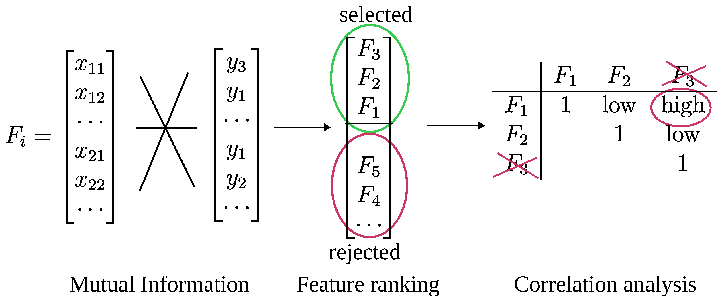
The workflow of the algorithm is depicted in Figure 2.
The Chi-Square ( χ 2 ) test is another widely used filter method for assessing the statistical dependence between a categorical feature and a categorical target variable. It evaluates whether the observed frequency distribution of feature values across target classes significantly deviates from the expected distribution under the assumption of independence. The Chi-Square statistic is defined as
χ 2 = i = 1 r j = 1 c O i j E i j 2 E i j ,
where O i j and E i j represent the observed and expected frequencies for category i and class j, respectively, and r and c denote the number of feature categories and target classes. Higher χ 2 values indicate a stronger association between the feature and the target, suggesting that the feature is more informative for classification.
While maximum relevance and Chi-Square focus on selecting features that are highly associated with the target variable, they do not account for redundancy among features. Including multiple features that are strongly correlated with each other may lead to overfitting and reduced model generalisability. To address this, we compute pairwise correlations between features:
c i j = corr ( F i , F j ) , for i j .
It allows the application to use methods such as maximum relevance, minimum redundancy (mRMR), where the goal is to select features that are individually relevant to the target while being minimally correlated with each other. Such strategies improve the diversity and predictive power of the selected feature subset.

3.2.2. Wrapper Methods

Wrapper algorithms evaluate subsets of features by using a specific ML algorithm, iteratively adding or removing features based on model performance. The wrapper methods usually achieve higher scores (e.g., accuracy, F1 score) than filter methods because they consider the interaction between features and the model. However, wrapper methods are computationally expensive, especially for large datasets, as they require multiple model evaluations.
One of the wrapper-based algorithms is Weighted KMeans (WKMeans), which is based on KMeans. The latter is a classical and popular clustering algorithm. For a given dataset Y, KMeans outputs a disjoint set of clusters S = { S 1 , S 2 , . . . , S K } . Each cluster S i S has a centroid c i C . The centroid c i should strive to minimise the sum of distances to all data points x i belonging to a cluster S i . Thus, c i is a good general representation of S k . KMeans partitions a dataset Y into K clusters by iteratively minimising the intra-cluster distance between data points x i Y and their corresponding centroids c k C . The optimisation objective is expressed as:
min W ( S , C ) = k = 1 K i S k v V d ( x i v , c k v ) ,
where V denotes the set of features describing each data point x i X .
The algorithm minimises the sum in (9) in three iterative steps until convergence. First, the algorithm randomly selects K data points from Y as the initial centroids c 1 , c 2 , , c K . Second, each data point x i X is assigned to the cluster S k associated with the nearest centroid. If the cluster assignments remain unchanged, the algorithm terminates and returns S and C. Otherwise, in the third step, each centroid c k C is updated as the mean of the points assigned to its cluster S k . Notably, this optimisation is NP-hard even for K = 2 [38].
In [39], Huang et al. introduced the WKMeans algorithm. WKMeans adds a weight w v β to the feature v distance in the function specified in (9).
W ( S , C , w ) = k = 1 K i S k v V w v β d ( x i v , c k v ) .
Similarly to (9) and (10) is minimised in iterations, and the parameters S, C, and w are updated one at a time. Assuming β > 1 , during the iteration, w v is updated as follows [39]:
w v = 0 , if D v = 0 1 j = 1 h D v D j 1 β 1 , if D v 0 ,
where
D v = k = 1 K i S k d ( x i v , c k v ) ,
and h is the number of features where D v 0 . In our experiment, we set β = 2 . For the discussion of possible consequences of different values for this parameter, see [39]. For β = 2 , the Equation (11) becomes
w v = 0 , if D v = 0 1 j = 1 h D v D j , if D v 0 .
When D v is small in comparison to other feature distances D j , j = 1 h , the weight w v increases. In other words, if feature v exhibits relatively low dispersion, it is more likely to form clusters; therefore, we increase its significance. Consequently, the weight of the feature in (13) also increases. As a result, the cluster centroid c v for a given k cluster should be adjusted more precisely compared to features with lower weights to minimise the equation. We can visualise this concept in Figure 3 for two exemplary features, v x and v y .
For our experiments, we adapted the implementation of WKMeans from [39].
Another wrapper-based approach applied in this study is Sequential Forward Selection (SFS), which incrementally builds an optimal subset of features by starting from an empty set and iteratively adding the feature that maximises the model performance. At each iteration, the candidate feature f j is added to the current subset F t , and the updated set F t + 1 = F t { f j } is evaluated. The evaluation is performed by training an SVM with a linear kernel on the given feature subset and computing the score on a validation set. The feature providing the highest improvement in the metric is retained, and the process repeats until a stopping condition is met. Formally, if S ( F ) denotes the score obtained by the model trained on feature subset F, the feature selected at step t is given by:
f * = arg max f F F t S ( F t { f } ) ,
where F is the full set of available features. The algorithm terminates when | F t | = k or when max f S ( F t { f } ) S ( F t ) < ϵ for a predefined tolerance ϵ .

3.2.3. Embedded Method—LassoNet

Unlike filter or wrapper approaches, embedded methods learn which features are most relevant during training, embedding feature selection within the model itself. This integration combines the advantages of both filter and wrapper methods, often resulting in improved generalisation and performance, as feature importance is assessed within the context of model optimisation. However, these methods often rely on more complex algorithms, which can make the results harder to interpret.
LassoNet (Least Absolute Shrinkage and Selection Operator) is a feature filter method that combines an ANN with Lasso regression. Lasso is a linear regression technique that incorporates L1 regularisation [27]. The regularisation term in Lasso promotes sparsity by driving some model coefficients to zero, effectively performing feature selection. This characteristic makes Lasso particularly suitable for identifying the most informative features within a dataset.
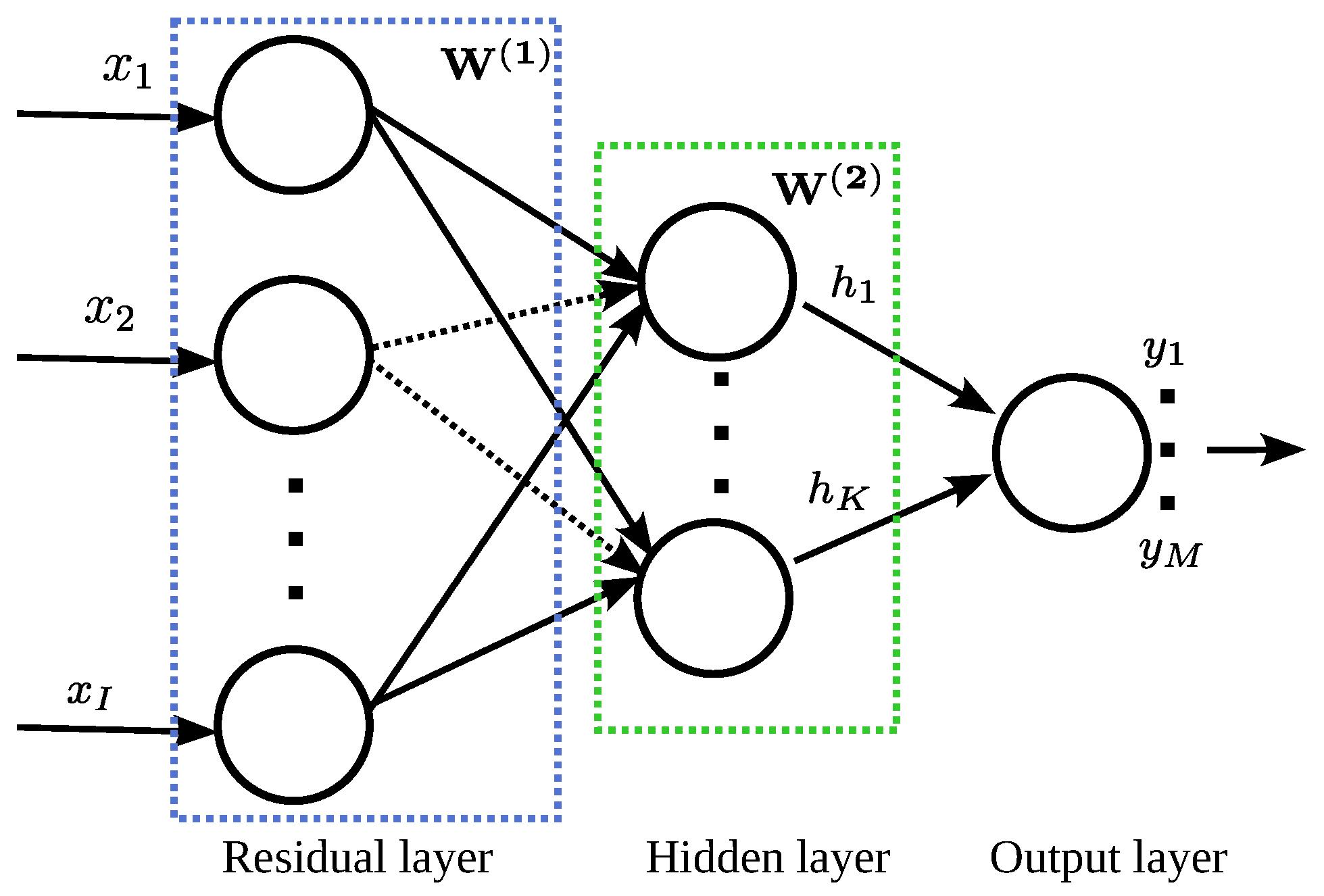
LassoNet operates on input vectors x R I , which are first processed through a weight matrix W ( 1 ) R K × I and a bias vector b ( 1 ) R K , connecting the input layer to the hidden layer. The hidden layer is subsequently linked to the output layer via the weight matrix W ( 2 ) R M × K and the corresponding bias vector b ( 2 ) R M , as illustrated in Figure 4. Let f denote the activation function (e.g., sigmoid, ReLU). The hidden layer activation h is then computed as
h = f ( W ( 1 ) x + b ( 1 ) ) ,
where h R K is the output of the hidden layer. The network’s output y is computed as
y = f ( W ( 2 ) h + b ( 2 ) ) ,
where y R M is the output of the network. The operation W ( 2 ) h + b ( 2 ) computes the weighted sum of hidden layer outputs plus the bias.
To optimise the parameters Θ = { W ( 1 ) , W ( 2 ) , b ( 1 ) , b ( 2 ) } for a given set of N training samples { x n , y true n } n = 1 N , the mean square error is used as the cost function,
MSE = 1 N i = 1 N y ( i ) y true ( i ) 2 ,
where y true ( i ) is the true target output for the ith training example, N is the number of training examples, and · denotes the Euclidean norm (or L2 norm).
What distinguishes LassoNet from a traditional network, is a penalty term added to the loss function that incorporates the feature selection mechanism. The total cost function J that combines the original cost (15) and the penalty function can be expressed as:
J ( θ ) = MSE + λ W ( 1 )
The penalty function encourages sparsity in the input layer, which can be interpreted as feature selection, by promoting many weights to be zero. This process is called Lasso regularisation. Regularisation allows the neural network to learn not only the mapping from inputs to outputs but also to select relevant features by penalising the model’s complexity. The penalisation is regulated by the λ parameter, which controls the strength of the penalty applied to the weights.
A batch gradient descent algorithm is used to minimise (15). Starting from an arbitrary initial value θ 0 , the gradient method updates the parameters iteratively as follows:
θ n + 1 = θ n η J E ( θ ) θ , n = 1 , 2 ,
where η > 0 is the learning rate.
For the experiments, we used the implementation described in [27].

3.3. Representation Learning-Based Approach

In addition to the classical filter, wrapper, and embedded feature selection methods, a modern representation learning approach was incorporated into the comparison to provide a state-of-the-art baseline. The proposed method combines a deep autoencoder with an SVM classifier, referred to as AE + SVM. An autoencoder is a type of feed-forward neural network trained to reconstruct its input, thereby learning a compressed representation in a latent space. It consists of two components: the encoder f θ , which maps an input vector x R n to a lower-dimensional latent representation z R m ( m < n ), and the decoder g ϕ , which reconstructs the input from z . The network is trained by minimising the reconstruction loss:
L rec ( θ , ϕ ) = 1 N i = 1 N x i g ϕ f θ ( x i ) 2 2 ,
where N is the number of training samples. After training, the encoder is used to transform the original features into the latent representation z , which captures the most salient patterns in the data while reducing noise and redundancy. These latent features are then used as input to an SVM with a linear kernel for supervised classification. This approach benefits from the autoencoder’s ability to learn non-linear feature transformations while leveraging the SVM’s strong generalisation performance in high-dimensional spaces.

4. Experiment and Its Results

The workflow commenced with the acquisition of network traffic, followed by its processing and conversion into a structured text format. In the subsequent step, the processed data were input into the three feature selection algorithms types under study: filter, wrapper, and embedded. In the case of the filter approach, we manually connected its output to the KMeans algorithm. In the case of the remaining two, clustering was an integral part, and no additional clustering techniques were needed. Then, we analysed the obtained clusters using the precision, recall, and F1 scores. The precision and recall are defined as:
( P ) recision = TP TP + FP ,
( R ) ecall = TP TP + FN ,
where a true positive (TP) corresponds to a case where a sample is correctly identified as belonging to a given class, while a true negative (TN) indicates a correct rejection of a sample from that class. Conversely, a false positive (FP) occurs when an instance is wrongly assigned to a class, and a false negative (FN) occurs when a sample belonging to the class is missed. The F1 score is defined as:
F 1 = 2 × Precision × Recall Precision + Recall ,
where precision is the fraction of predicted pairs that are correct (i.e., both in the same cluster and same class), and recall is the fraction of true pairs identified by the clustering algorithm. The following sections provide a description of each step in the process.

4.1. Characteristics of Network Traffic

Video streaming platforms commonly rely on Dynamic Adaptive Streaming over HTTP (DASH), a widely adopted standard for delivering video content. In this approach, a single video is encoded into several versions of different resolutions, such as 480p, 720p, or 1080p, and divided into discrete segments. A Media Presentation Description (MPD) file accompanies the video content, specifying available resolutions and segment organisation. Upon playback, the video client downloads the MPD file and begins requesting segments. To ensure smooth playback, the client continuously monitors network conditions (e.g., bandwidth, latency, and jitter) and adapts segment quality accordingly.
Streaming providers tailor their delivery mechanisms to handle diverse and fluctuating network conditions. Typically, the quantity of data transferred during the initial buffering phase differs significantly from that during continuous playback. For example, YouTube clients may download several segments in a burst, leading to variability in traffic volumes and inter-segment timing. These adaptive behaviours cause even the same video to generate different traffic patterns [40]. As a result, DASH-based video traffic reflects platform-specific characteristics shaped by choices in segment duration, encoding methods, bitrate adaptation logic, and caching strategies, all of which contribute to unique statistical patterns in network traces.
We analysed video traffic generated by three popular platforms, YouTube, Netflix, and Amazon Prime Video (hereinafter referred to as Amazon), which account for a substantial portion of global Internet traffic [41]. Two video resolutions were selected for the study: 720p and 1080p. The former corresponds to 1280 × 720 pixels and serves as the baseline for high-definition video, commonly referred to as Standard HD. This resolution is suitable for small-screen devices such as smartphones, tablets, and entry-level cameras. The latter, known as Full HD, has a resolution of 1920 × 1080 pixels and is widely used on larger displays, including televisions, computer monitors, and projectors. To reflect real-world usage scenarios, we collected the 720p traffic traces in a 5G mobile network environment and the 1080p traces in a stable wired network environment. The details of the collected traffic traces are summarised in Table 1.
We obtained video traffic traces using Wireshark. Each capture spanned two hours and was sampled at one-second intervals. After recording, we converted Wireshark’s files into a data frame representing throughput over time. Although some datasets related to streamed video are publicly available [42], video services frequently update their streaming algorithms to adapt to evolving user behaviour, technology, and content trends [22,41]. Consequently, data collected several years ago may be outdated, and their statistical characteristics differ from current traffic. To avoid misleading conclusions, we therefore acquired our own up-to-date traffic datasets.
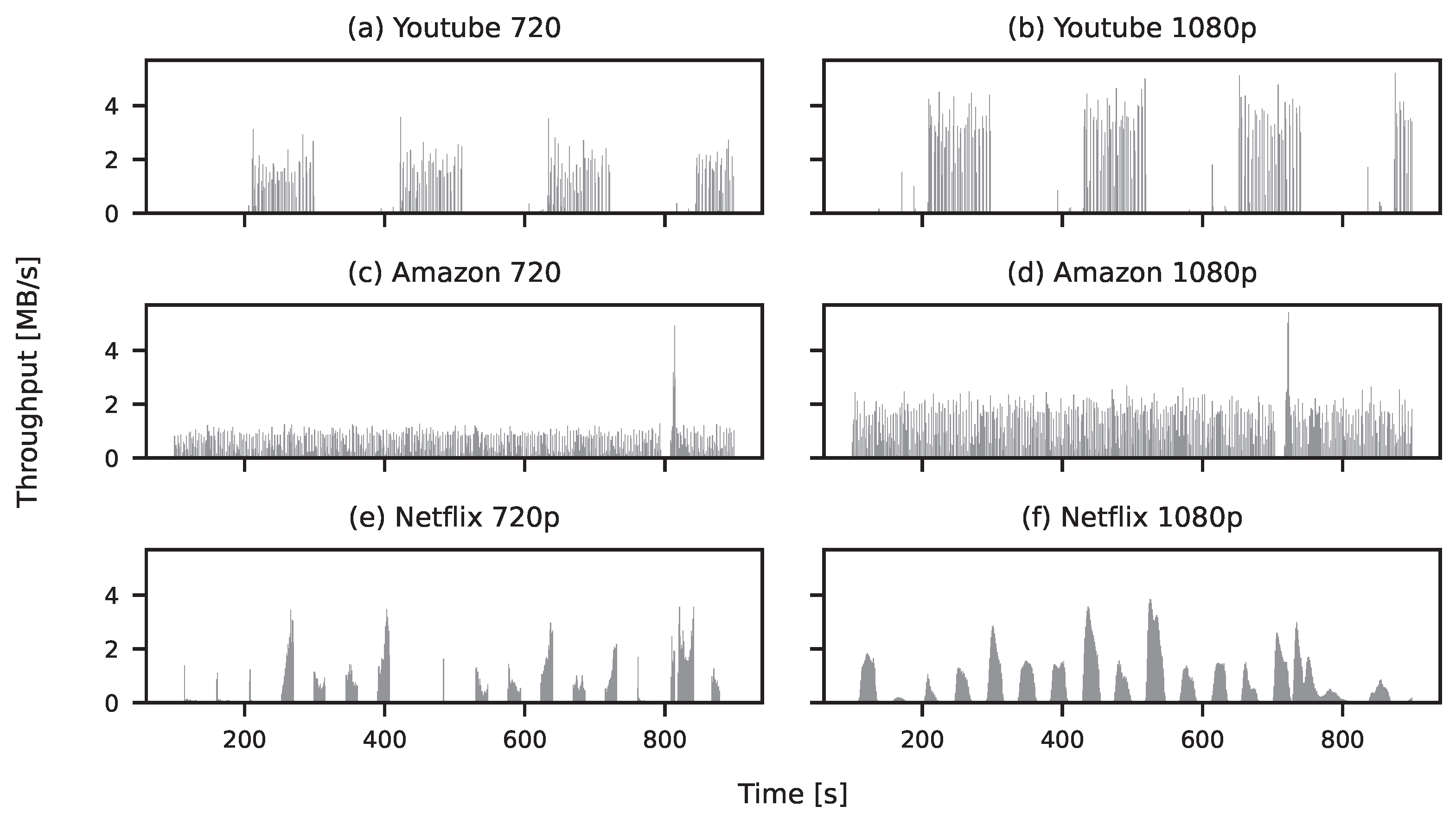
The individual traces generated by video streaming exhibit varied patterns, as shown in Figure 5. These patterns depend on how the video player manages data downloads. Traffic patterns for both YouTube and Netflix reveal a characteristic ON/OFF behaviour, marked by alternating bursts of data transfer and idle periods. Notably, YouTube exhibits longer durations in both the data transmission and inactivity phases compared to Netflix, reflecting differences in how each platform manages buffering and segment delivery. The traffic generation process for Amazon also exhibits two states, characterised by higher or lower traffic intensity. According to [41], YouTube and Netflix have longer ON intervals. Consequently, these services download larger volumes of data in each burst compared to Amazon. However, despite the shorter duration of each cycle, Amazon maintains a comparable overall data volume by increasing the frequency of its transmission bursts within the same time frame.
For YouTube, this ON/OFF structure is consistent regardless of video resolution. Both 720p and 1080p resolutions (Figure 5a and Figure 5b, respectively) exhibit clear ON/OFF patterns with well-defined boundaries. Similarly, Amazon’s statistical characteristics remain stable across resolutions. Compared to the 720p version (Figure 5a,c), the 1080p stream (Figure 5d), shows somewhat increased traffic intensity. The ON and OFF periods for Netflix have irregular lengths, and the ON periods also have different throughput. Compared to 720p, presented in Figure 5e, for 1080p, the ON periods last longer but do not necessarily have higher throughput; see Figure 5f. To accommodate a higher bit rate while remaining within transmission constraints, the OFF periods are minimised, reducing interruptions in data transmission.

4.2. Extracted Features

For feature extraction, we employed tsfresh (Feature Extraction based on Scalable Hypothesis tests) [43], which, as reported in [43], computes a total of 794 features from time series data. Furthermore, it includes statistical, spectral, and information-theoretic features, offering a comprehensive characterisation of time series data.
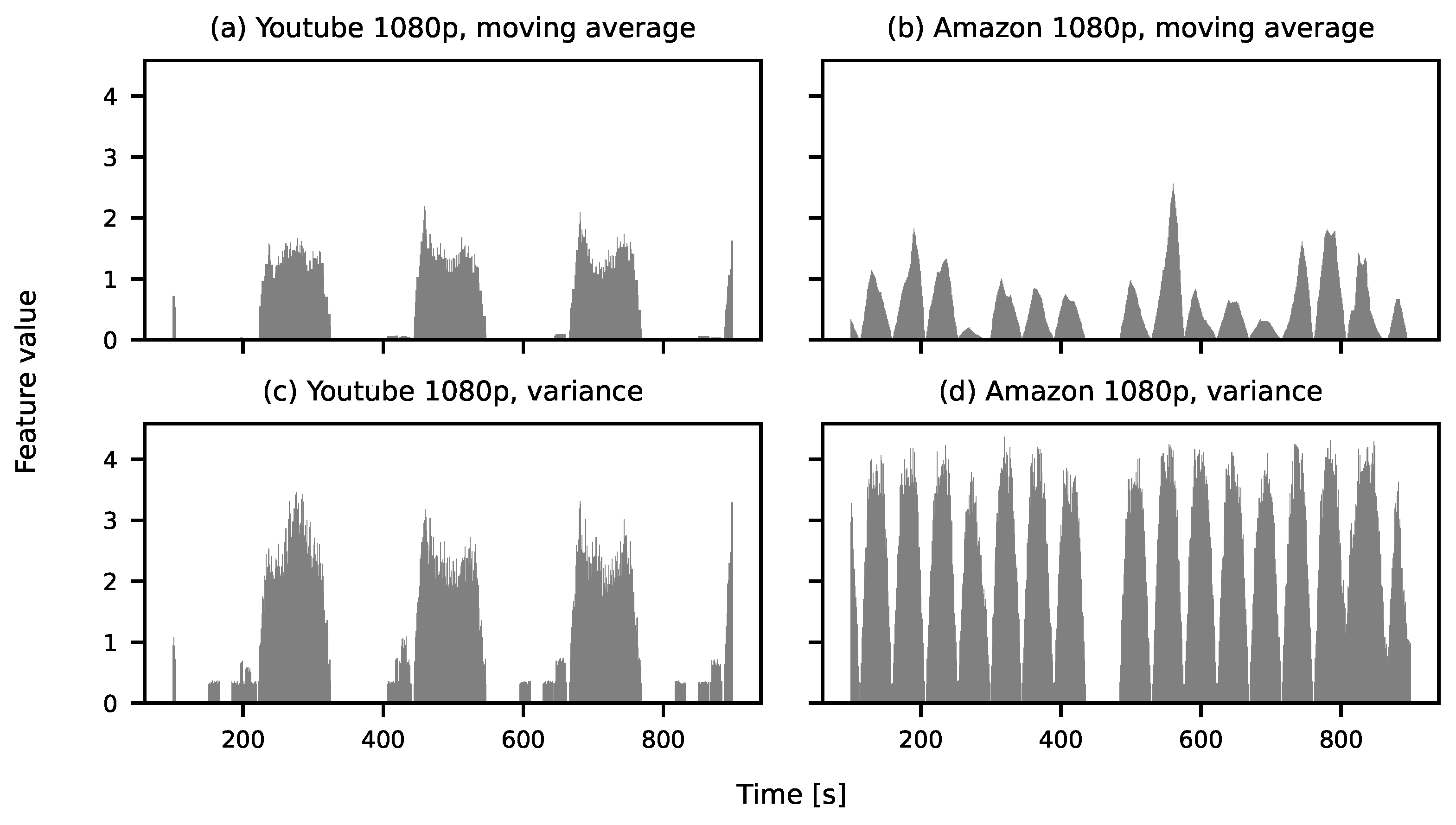
Figure 6 presents the temporal characteristics of two features: the moving average and the variance. For YouTube traffic, shown in Figure 6a,c, distinct cycles are observable in both features. This directly reflects the cyclical nature of the traffic generated by this service. In contrast, the moving average for Amazon traffic appears more irregular, as illustrated in Figure 6b. However, when considering the variance feature (Figure 6d), cyclical behaviour becomes apparent once again.
The observations illustrated in Figure 6 suggest that the visibility of structural patterns depends on the selected feature. Some traffic characteristics which may not be evident in the original signal become clearer through feature extraction. Consequently, feature extraction not only reduces the amount of information and filters out noise but also enhances the interpretability and statistical understanding of the data.
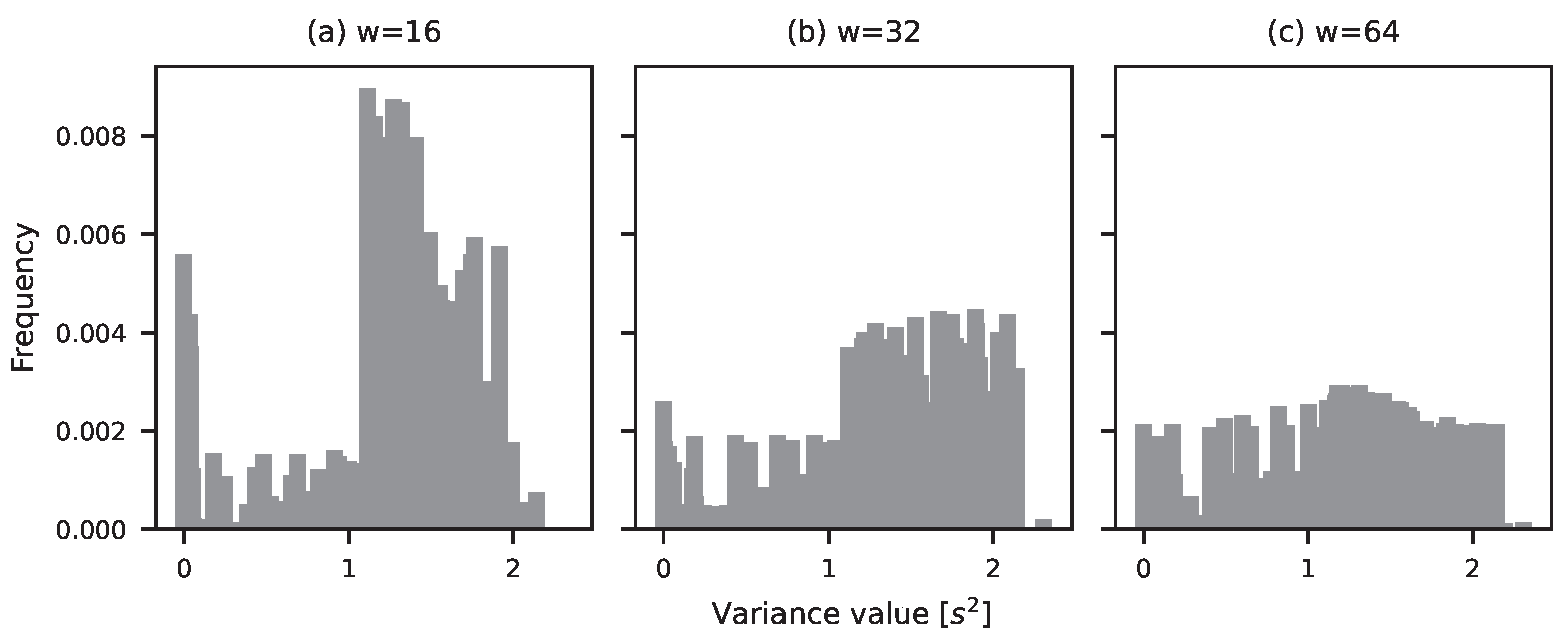
The characteristics of extracted features change with the quantity of gathered data. For example, modifying the size of the sliding window w in (2) affects the distribution of the variance feature, as illustrated in Figure 7. Specifically, as the sliding window length increases, the histogram of the variance feature becomes increasingly flattened. This flattening indicates that the spread (or variability) of variance values grows with more data. In other words, local variability becomes more pronounced at larger time scales, suggesting that the time series exhibits greater heterogeneity when observed over longer windows. Importantly, this implies that increasing the window length does not necessarily smooth the data, at least in terms of variance. Instead, the results indicate that the video traces exhibit non-stationary behaviour, where adding more data introduces greater variability. This is often the result of seasonality or structural breaks within the time series.

4.3. Clustering Performance

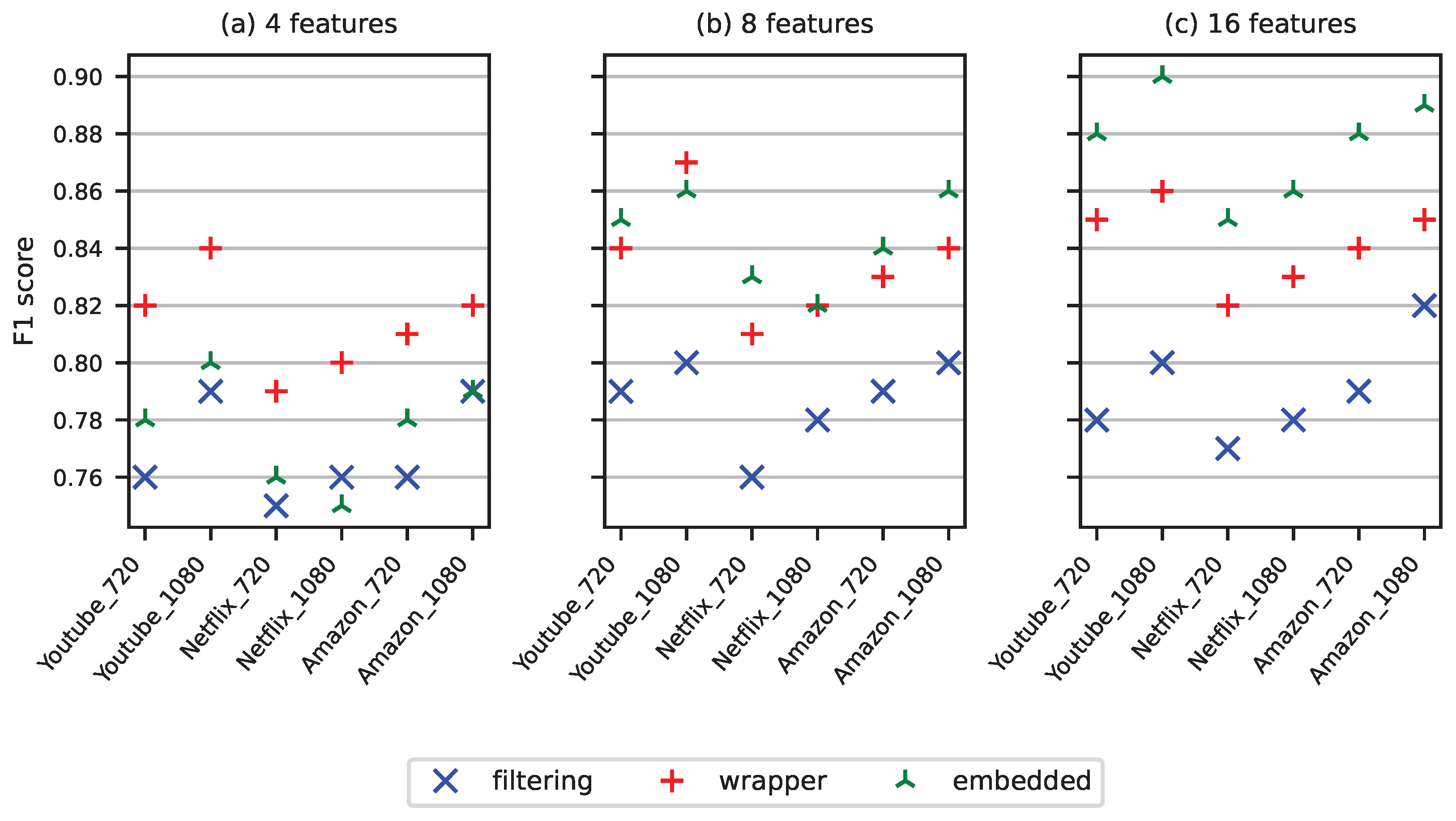
In Figure 8, we compare the three types of feature selection approaches described in Section 3.2: filter, wrapper, and embedded, represented by three algorithms: MI, WKMeans, and Lassonet, across six video traces. When the algorithms operate on a limited number of features (set to four), as shown in Figure 8a, the traffic generated by YouTube is the most easily distinguishable, followed by Amazon. Netflix traffic receives the lowest F1 score, which may be attributed to its higher degree of irregularity. In all cases, traffic generated by 1080p video yielded higher classification scores. This can be explained by the fact that 1080p traffic was typically captured in a more stable environment and exhibited a more regular structure compared to 720p traffic, which was collected over a mobile network.
When comparing the individual algorithms, we observed that for 1080p videos from YouTube and Amazon, all three methods achieved comparable results, which were in the range between 0.74 and 0.84. For traffic generated by 720p videos from these same services, the filter method performed slightly worse than the wrapper and embedded approaches, which produced similar F1 scores. A similar trend was observed for Netflix’s 1080p and 720p traffic, where the filter approach again underperformed due to the lower predictability of the data, while the other two methods yielded higher and more stable results.
Increasing the number of features to eight led to improved F1 scores across all categories, as shown in Figure 8b. The most significant improvement was observed for the wrapper algorithm, followed by the embedded approach, with the smallest gain for the filter method. However, the final results also depended on the type of video trace. In particular, the most notable improvements occurred for traces generated in mobile environments. Mobile traffic tends to exhibit higher entropy, so adding more features enhances clustering performance. Among the video services, YouTube showed relatively modest improvements. The highest increase in F1 score was observed for Netflix, followed by Amazon. The latter two traces had higher entropy than that of YouTube; thus, the algorithms could leverage more informative dimensions to identify similarities and differences among the traces.
Further increasing the number of features from 8 to 16 continued to improve performance, though the average gain was smaller compared to the transition from 4 to 8 features, as illustrated in Figure 8c. The highest overall scores were achieved by the embedded algorithm, followed by the wrapper and filter ones. The embedded approach, which is based on ANNs and heuristic optimisation, performs best when a relatively large quantity of data is available.
With regard to video resolution, 720p streams showed the most significant increase in F1 score compared to 1080p. Once again, the largest improvement was seen in Netflix traces, followed by Amazon and YouTube. As in the previous case with eight features, the inclusion of additional data enabled better clustering of traffic with higher irregularity.
The interpretation of these results is as follows: video traces that are relatively easy to classify—those with lower entropy and high regularity—can be effectively identified using simpler algorithms such as filter or wrapper methods. These methods require fewer data and can operate efficiently with a limited number of features, such as four. However, as the entropy and complexity of the video traces increase, more advanced methods like the embedded approach become necessary. This approach requires a larger feature set and a greater volume of data to capture the underlying patterns effectively. In our experiments, the embedded method achieved the highest F1 score when operating with 16 features.
In Table 2, we present an extended comparison of feature selection, including precision (18), recall (19) and two additional algorithms: Chi-Square test, presented in Section 3.2.1, and Sequential Forward Selection, presented in Section 3.2.2. Furthermore, we compare them with a representation learning-based approach represented by Autoencoder+SVM, described in Section 3.3. The best overall performance was achieved by the embedded approach. It consistently produced the highest or near-highest F1 scores across all traces, showing a good balance between precision and recall. This indicates that the algorithm was able to extract compact and discriminative feature representations that generalised well across different video services and resolutions. Wrapper methods (WKMeans, SFS) came next, usually outperforming the pure filter approaches and, in a few cases, also outperforming the embedded approach. Also, the wrapper methods achieved comparable levels of precision and recall across the evaluated algorithms, indicating that the models maintained a balanced trade-off between correctly identifying positive samples and avoiding false negatives. Between the two wrapper methods, the superiority of one over the other depended on the dataset, as each showed stronger performance on different video traces. Autoencoder+SVM performed competitively, often close in performance to wrapper approaches but with slightly less symmetry between precision and recall. Filter methods (mutual information and Chi-Square) showed the weakest results overall. Between the two, mutual information generally achieved higher F1 scores than Chi-Square, though both were clearly below wrapper and autoencoder methods in performance. This suggests that simple statistical association tests are insufficient for capturing the complex relationships in video traffic data. The worst performer was the Chi-Square Test, which consistently gave the lowest F1 scores.
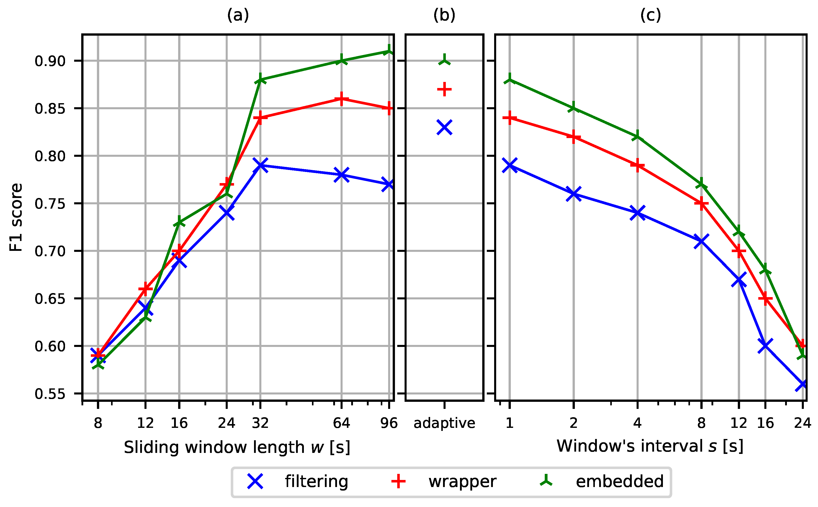
In Figure 9, we present a sensitivity analysis that considers different values of the sliding window length w and the interval between windows s, as defined in (2).
The window length parameter w is used to segment continuous traffic into samples, which serve as the basic units for the classification task. Variations in w affect the size of each sample, the quantity of included network flow data, and consequently the classification performance, as shown in Figure 9a. We evaluated the model’s prediction metrics across multiple values of w ( w { 8 , 12 , 16 , 24 , 32 , 64 , 96 } ). As shown in Figure 9a, the F1 score generally increased with a larger window length. However, the performance plateaued at different values depending on the algorithm used. For example, the filter algorithm reached its peak F1 score at a window length of 32 s, the wrapper algorithm peaked at 48 s, and the embedded approach based on the Lasso network only achieved its highest score at 96 s.
In Figure 9b, the window length was adaptively set to w according to (3). Overall, the adaptive window improved classification performance compared to fixed lengths. The filter method showed the largest gain, increasing by approximately 0.05 percentage points, while the wrapper method improved by 0.01 percentage points. The embedded method did not benefit from adaptivity, exhibiting a slight decrease of 0.01 percentage points in F1 score.
Regarding the window interval parameter s, which defines the step size between subsequent windows, we observed that increasing s beyond four led to a rapid decline in classification performance, as illustrated in Figure 9c. The steepest performance drop and lowest scores were observed for the filter method. The wrapper algorithm performed slightly better, showing a more gradual decline. The embedded algorithm proved most robust, maintaining a higher F1 score for almost all cases.
Table 3 presents the relative execution times for the MI, WKMeans, and LassoNet algorithms. As expected from the algorithmic descriptions, the filter method was the fastest, requiring less than 1% of the total time allocated to all three approaches. This is due to its simplicity: it does not involve model training and relies solely on relatively fast statistical computations.
In contrast, the wrapper approach was significantly more time-consuming, accounting for approximately 62% of the total execution time. This method involves training the model multiple times, each time using different subsets of features. For each subset, it computes triple sums as defined in (10), which further increases the computational cost.
The embedded method, based on the LassoNet architecture, accounted for the remaining 38% of the execution time. Its runtime primarily depends on the cost of training the neural network and the number of features included in the learning process.

4.4. Discussion

The analysis demonstrates that the proposed algorithms exhibit varying levels of performance in the context of video motion classification. The filter-type algorithms generally yield the lowest F1 score among the evaluated methods; however, they perform relatively well when only a limited quantity of data is available. They are also the fastest in terms of execution time. Notably, increasing the number of features does not significantly enhance their F1 score. This limitation may stem from the inherent constraints of the KMeans clustering algorithm used in conjunction with this method. In high-dimensional spaces, distance metrics tend to lose their discriminative power, as data points become increasingly equidistant. Consequently, the clustering contrast is diminished, reducing overall effectiveness. Despite its lower F1 score, the filter approach consistently identifies video traffic types correctly in the majority of cases. Given its low computational cost and acceptable performance, it can serve as a practical baseline or prototype solution for traffic engineering applications.
The highest classification scores were achieved by the embedded-type algorithm based on LassoNet. However, unlike the filter approach, that method requires more training data and greater computational resources to yield reliable results. For short sliding windows, its performance was comparable to that of the filter algorithms. It also demonstrated the highest resilience to increases in the window interval parameter, as presented in Figure 9c. Moreover, when data are limited, the model may overfit to noise or spurious patterns, potentially selecting features that are not genuinely relevant to the classification task. The introduction of an adaptive window length does not lead to performance improvements, as LassoNet inherently regularises feature relevance and, to some extent, automatically determines the effective quantity of data needed for decision-making. To enhance its F1 score, a hybrid approach could be employed, wherein features are first pre-selected using the filter method before being passed to the neural network. Additionally, techniques such as k-fold cross-validation may help mitigate overfitting by ensuring that selected features generalise well across different subsets of the data.
The wrapper-type algorithms serve as a middle-ground approach: they require more data than the filter method, but less than the embedded approach. As shown in Figure 8, WKMeans delivers strong performance even with only four features and short sliding windows, see Figure 9a. Similar to the embedded method, the wrapper algorithms can also benefit from a two-step process, where an initial filter step removes irrelevant features, thereby improving the effectiveness and efficiency of the feature selection process.
While the above five algorithms provide a structured comparison across methodological classes, the reliance on one or two representative algorithms per category introduces certain limitations. Specifically, each algorithm embodies its assumptions, biases, and sensitivities to data properties, which may not fully reflect the strengths or weaknesses of the broader class it represents. For example, MI may not capture more complex interactions between features and target labels. Chi-Square detects whether an association exists but does not quantify the amount of shared information like MI. Similarly, the performance of the wrapper method is tied to the characteristics of the clustering algorithm. For example, WKMeans is sensitive to the initial placement of centroids, which can cause convergence to local minima. In turn, SFS is a greedy wrapper method that iteratively evaluates the addition of each feature to the selected set. For high-dimensional datasets, this requires training and evaluating the model many times, which can be more accurate but slower than for WKMeans.
Lastly, although LassoNet effectively integrates feature selection with model training, it may not generalise to all embedded-based approaches, particularly those using alternative regularisation strategies or network architectures. As such, the conclusions drawn from these comparisons should be interpreted with caution, and future work could expand the analysis to include multiple algorithms within each category to improve generalisability and robustness.
The above studies were limited to a narrow segment of network traffic, namely, DASH video streams. Furthermore, these video streams were transmitted in relatively stable network conditions. This can limit the generalisability of the trained models and their ability to accurately classify traffic patterns in more dynamic or degraded network environments. Thus, future work should incorporate traces collected under diverse and unstable conditions to ensure broader comparison of the feature extraction algorithms.
Another limitation is the adoption of a constant time window length w (2) for extracted features. A fixed window size applies a uniform length across the entire time series, which simplifies implementation and ensures consistency of feature representation. However, it may fail to capture important local variations in non-stationary or multi-scale data. In contrast, a variable window size dynamically adapts to the temporal structure of the data, allowing better alignment with patterns such as bursts, trends, or periodicity. This approach can improve feature relevance, see Figure 9b, but it introduces additional complexity in terms of segmentation strategy and model interpretability.
Similar considerations can be applied to the interval s between windows (2). A fixed interval ensures uniform coverage of the time series, which simplifies the extraction process and produces a regular number of feature vectors. However, it may introduce redundancy when the interval is small or miss important transitions when the interval is large. Conversely, a variable interval adapts the step size based on signal characteristics, e.g., detecting changes in variance or thresholds, to better align windows with meaningful events. While this can improve sensitivity to dynamic behaviour, it increases computational complexity and may lead to irregular feature representations that require additional normalisation or alignment during modelling.
While deep learning approaches are widely adopted in traffic classification tasks, our findings suggest that feature engineering and feature selection remain highly relevant research directions. Deep learning models are often designed as general-purpose learners and require large annotated datasets, substantial computational resources, and significant retraining effort when network conditions or protocols change. In contrast, feature engineering methods can provide more specialised, efficient, and interpretable solutions, which are crucial in practical deployments. For example, a lightweight model based on carefully engineered features can be more suitable for real-time traffic monitoring on network devices with limited computational capabilities, where retraining a deep model would be infeasible.
An additional advantage is that feature-based approaches adapt more easily to the newest forms of adaptive video streaming, such as evolving DASH implementations. Because engineered features are interpretable, changes introduced in new protocol versions can be quickly reflected in updated feature sets without the need for expensive retraining. This flexibility allows simple models to remain effective in practice and ensures that they keep pace with protocol updates, where black-box deep learning models may lag behind.
From a systems perspective, having models that are lightweight, interpretable, and easy to update ensures better maintainability and faster adaptation to new streaming services or protocol changes. Thus, the continued exploration of feature engineering not only complements advances in deep learning but also provides robust and resource-efficient alternatives for traffic classification.

5. Conclusions

This study presented a comparative analysis of three feature selection strategies for video traffic classification: filter, wrapper, and embedded. Using real-world traces from YouTube, Netflix, and Amazon Prime Video across different resolutions and network conditions, we examined how each method performed in terms of classification accuracy and computational efficiency.
Our findings show that filter methods, while computationally lightweight, offer modest accuracy and are best suited for low-entropy traffic or scenarios with limited data availability. Wrapper methods improve classification performance by evaluating feature subsets in conjunction with clustering, but they incur significantly higher computational costs. Embedded methods, particularly those based on LassoNet, demonstrate the highest F1 scores, especially when applied to high-entropy or mobile-collected traces with a larger number of features. However, these methods require substantial training data and processing time.
We also observed that increasing the number of features benefited all methods, especially for irregular and high-entropy traffic, although the performance gains diminished beyond a certain point. Sensitivity analysis revealed that both sliding window size and interval affected classification performance and should be carefully tuned.
While our methodology provides insights into the trade-offs between different feature selection strategies, the conclusions are based on representative algorithms for each category and a specific type of traffic, namely, DASH videos. To improve generalisability, future research should extend this analysis to broader traffic types, diverse network environments, and a wider selection of algorithms within each feature selection class. Additional experiments involving different algorithms for variable window sizes and adaptive interval strategies may also enhance model robustness and applicability to non-stationary traffic patterns.
Beyond the direct comparison of algorithms, our work confirms that feature engineering and simple models remain highly relevant, even in the era of deep learning. While the latter are powerful and general, they require extensive resources, large labelled datasets, and retraining when protocols evolve. In contrast, feature-based methods are lightweight, interpretable, and more easily adaptable to new streaming standards such as evolving DASH implementations. These qualities make them practical for real-time deployment on constrained network devices, and they can provide specialised efficiency that complements the generality of deep learning.

Funding

The work was carried out within the statutory research project of the Silesian University of Technology, Department of Computer Networks and Systems.

Institutional Review Board Statement

Not applicable.

Informed Consent Statement

Not applicable.

Data Availability Statement

Publicly available datasets were analysed in this study. These data can be found at https://github.com/arczello/video_traces, accessed on 27 July 2025.

Conflicts of Interest

The author declares no conflict of interest.

References

  1. Wang, Z.; Fok, K.W.; Thing, V.L. Machine learning for encrypted malicious traffic detection: Approaches, datasets and comparative study. Comput. Secur. 2022, 113, 102542. [Google Scholar] [CrossRef]
  2. Akbari, I.; Salahuddin, M.A.; Aniva, L.; Limam, N.; Boutaba, R.; Mathieu, B.; Moteau, S.; Tuffin, S. Traffic classification in an increasingly encrypted web. Commun. ACM 2022, 65, 75–83. [Google Scholar] [CrossRef]
  3. Shen, M.; Ye, K.; Liu, X.; Zhu, L.; Kang, J.; Yu, S.; Li, Q.; Xu, K. Machine Learning-Powered Encrypted Network Traffic Analysis: A Comprehensive Survey. IEEE Commun. Surv. Tutor. 2023, 25, 791–824. [Google Scholar] [CrossRef]
  4. Li, Z.; Chen, J.; Ma, X.; Du, M.; Zhang, Z.; Liu, Q. A robust and accurate encrypted video traffic identification method via graph neural network. In Proceedings of the 2023 26th International Conference on Computer Supported Cooperative Work in Design (CSCWD), IEEE, Rio de Janeiro, Brazil, 24–26 May 2023; pp. 867–872. [Google Scholar]
  5. Aouedi, O.; Piamrat, K.; Hamma, S.; Perera, J.K.M. Network traffic analysis using machine learning: An unsupervised approach to understand and slice your network. Ann. Telecommun. 2022, 77, 297–309. [Google Scholar] [CrossRef]
  6. Cao, J.; Wang, D.; Qu, Z.; Sun, H.; Li, B.; Chen, C.L. An improved network traffic classification model based on a support vector machine. Symmetry 2020, 12, 301. [Google Scholar] [CrossRef]
  7. Yang, L.Y.; Dong, Y.N.; Tian, W.; Wang, Z.J. The study of new features for video traffic classification. Multimed. Tools Appl. 2019, 78, 15839–15859. [Google Scholar] [CrossRef]
  8. Gudla, R.; Vollala, S.; Srinivasa, K.G.; Amin, R. TCC: Time constrained classification of VPN and non-VPN traffic using machine learning algorithms. Wirel. Netw. 2025, 31, 3415–3429. [Google Scholar] [CrossRef]
  9. Wang, Z.; Ma, B.; Zeng, Y.; Lin, X.; Shi, K.; Wang, Z. Differential preserving in XGBoost model for encrypted traffic classification. In Proceedings of the 2022 International Conference on Networking and Network Applications (NaNA), IEEE, Urumqi, China, 3–5 December 2022; pp. 220–225. [Google Scholar]
  10. Gil, G.D.; Lashkari, A.H.; Mamun, M.; Ghorbani, A.A. Characterization of encrypted and VPN traffic using time-related features. In Proceedings of the 2nd International Conference on Information Systems Security and Privacy (ICISSP 2016), Rome, Italy, 19–21 February 2016; SciTePress: Setúbal, Portugal, 2016; pp. 407–414. [Google Scholar]
  11. Min, Z.; Gokhale, S.; Shekhar, S.; Mahmoudi, C.; Kang, Z.; Barve, Y.; Gokhale, A. Enhancing 5G network slicing for IoT traffic with a novel clustering framework. Pervasive Mob. Comput. 2024, 104, 101974. [Google Scholar] [CrossRef]
  12. Yao, Z.; Ge, J.; Wu, Y.; Lin, X.; He, R.; Ma, Y. Encrypted traffic classification based on Gaussian mixture models and hidden Markov models. J. Netw. Comput. Appl. 2020, 166, 102711. [Google Scholar] [CrossRef]
  13. Yang, L.; Dong, Y.; Wang, Z.; Gao, F. One-dimensional CNN Model of Network Traffic Classification based on Transfer Learning. KSII Trans. Internet Inf. Syst. 2024, 18, 420–437. [Google Scholar] [CrossRef]
  14. Krupski, J.; Graniszewski, W.; Iwanowski, M. Data Transformation Schemes for CNN-Based Network Traffic Analysis: A Survey. Electronics 2021, 10, 2042. [Google Scholar] [CrossRef]
  15. Ren, X.; Gu, H.; Wei, W. Tree-RNN: Tree Structural Recurrent Neural Network for Network Traffic Classification. Expert Syst. Appl. 2021, 167, 114363. [Google Scholar] [CrossRef]
  16. Zhao, Z.; Li, Z.; Jiang, J.; Yu, F.; Zhang, F.; Xu, C.; Zhao, X.; Zhang, R.; Guo, S. ERNN: Error-resilient RNN for encrypted traffic detection towards network-induced phenomena. IEEE Trans. Dependable Secur. Comput. 2023, 1–18. [Google Scholar] [CrossRef]
  17. Jenefa, A.; Sam, S.; Nair, V.; Thomas, B.G.; George, A.S.; Thomas, R.; Sunil, A.D. A robust deep learning-based approach for network traffic classification using CNNs and RNNs. In Proceedings of the IEEE 2023 4th International Conference on Signal Processing and Communication (ICSPC), Coimbatore, India, 23–24 March 2023; pp. 106–110. [Google Scholar]
  18. Du, Y.; He, M.; Wang, X. A clustering-based approach for classifying data streams using graph matching. J. Big Data 2025, 12, 37. [Google Scholar] [CrossRef]
  19. Olabanjo, O.; Wusu, A.; Aigbokhan, E.; Olabanjo, O.; Afisi, O.; Akinnuwesi, B. A novel graph convolutional networks model for an intelligent network traffic analysis and classification. Int. J. Inf. Technol. 2024. [Google Scholar] [CrossRef]
  20. Yang, T.; Jiang, R.; Deng, H.; Li, Q.; Liu, Z. Ae-dti: An efficient darknet traffic identification method based on autoencoder improvement. Appl. Sci. 2023, 13, 9353. [Google Scholar] [CrossRef]
  21. Narmadha, S.; Balaji, N. Improved network anomaly detection system using optimized autoencoder- LSTM. Expert Syst. Appl. 2025, 273, 126854. [Google Scholar] [CrossRef]
  22. Atashgahi, Z.; Liu, T.; Pechenizkiy, M.; Veldhuis, R.; Mocanu, D.C.; Schaar, M.v.d. Unveiling the Power of Sparse Neural Networks for Feature Selection. arXiv 2024, arXiv:2408.04583. [Google Scholar] [CrossRef]
  23. Tekin, N.; Acar, A.; Aris, A.; Uluagac, S.; Gungor, V.C. Energy consumption of on-device machine learning models for IoT intrusion detection. Internet Things 2023, 21, 100670. [Google Scholar] [CrossRef]
  24. Hoefler, T.; Alistarh, D.; Ben-Nun, T.; Dryden, N.; Peste, A. Sparsity in deep learning: Pruning and growth for efficient inference and training in neural networks. J. Mach. Learn. Res. 2021, 22, 1–124. [Google Scholar]
  25. Atashgahi, Z.; Sokar, G.; Van Der Lee, T.; Mocanu, E.; Mocanu, D.C.; Veldhuis, R.; Pechenizkiy, M. Quick and robust feature selection: The strength of energy-efficient sparse training for autoencoders. Mach. Learn. 2022, 111, 377–414. [Google Scholar] [CrossRef]
  26. van der Wal, P.R.; Strisciuglio, N.; Azzopardi, G.; Mocanu, D.C. Multilayer perceptron ensembles in a truly sparse training context. Neural Comput. Appl. 2025, 37, 15419–15438. [Google Scholar] [CrossRef]
  27. Lemhadri, I.; Ruan, F.; Abraham, L.; Tibshirani, R. LassoNet: A Neural Network with Feature Sparsity. arXiv 2021, arXiv:1907.12207. [Google Scholar] [CrossRef]
  28. Peng, H.; Fang, G.; Li, P. Copula for instance-wise feature selection and rank. In Proceedings of the Uncertainty in Artificial Intelligence, PMLR, Pittsburgh, PA, USA, 31 July–4 August 2023; pp. 1651–1661. [Google Scholar]
  29. Moslemi, A.; Jamshidi, M. Unsupervised feature selection using sparse manifold learning: Auto-encoder approach. Inf. Process. Manag. 2025, 62, 103923. [Google Scholar] [CrossRef]
  30. Ou, J.; Li, J.; Xia, Z.; Dai, S.; Guo, Y.; Jiang, L.; Tang, J. RFAE: A high-robust feature selector based on fractal autoencoder. Expert Syst. Appl. 2025, 285, 127519. [Google Scholar] [CrossRef]
  31. Nascita, A.; Aceto, G.; Ciuonzo, D.; Montieri, A.; Persico, V.; Pescapé, A. A Survey on Explainable Artificial Intelligence for Internet Traffic Classification and Prediction, and Intrusion Detection. IEEE Commun. Surv. Tutor. 2024. [Google Scholar] [CrossRef]
  32. Guerra, J.L.; Catania, C.; Veas, E. Datasets are not enough: Challenges in labeling network traffic. Comput. Secur. 2022, 120, 102810. [Google Scholar] [CrossRef]
  33. Papadogiannaki, E.; Ioannidis, S. A survey on encrypted network traffic analysis applications, techniques, and countermeasures. ACM Comput. Surv. (CSUR) 2021, 54, 1–35. [Google Scholar] [CrossRef]
  34. Liu, T.; Lu, Y.; Zhu, B.; Zhao, H. Clustering high-dimensional data via feature selection. Biometrics 2023, 79, 940–950. [Google Scholar] [CrossRef]
  35. Saisubramanian, S.; Galhotra, S.; Zilberstein, S. Balancing the tradeoff between clustering value and interpretability. In Proceedings of the AAAI/ACM Conference on AI, Ethics, and Society, San Jose, CA, USA, 21–23 October 2020; pp. 351–357. [Google Scholar]
  36. Salles, I.; Mejia-Domenzain, P.; Swamy, V.; Blackwell, J.; Käser, T. Interpret3C: Interpretable Student Clustering Through Individualized Feature Selection. In Proceedings of the International Conference on Artificial Intelligence in Education, Recife, Brazil, 8–12 July 2024; Springer: Berlin/Heidelberg, Germany, 2024; pp. 382–390. [Google Scholar]
  37. Amaldi, E.; Kann, V. On the approximability of minimizing nonzero variables unsatisfied relations in linear systems. Theor. Comput. Sci. 1998, 209, 237–260. [Google Scholar] [CrossRef]
  38. Aloise, D.; Deshpande, A.; Hansen, P.; Popat, P. NP-hardness of Euclidean sum-of-squares clustering. Mach. Learn. 2009, 75, 245–248. [Google Scholar] [CrossRef]
  39. Huang, J.Z.; Ng, M.K.; Rong, H.; Li, Z. Automated variable weighting in k-means type clustering. IEEE Trans. Pattern Anal. Mach. Intell. 2005, 27, 657–668. [Google Scholar] [CrossRef] [PubMed]
  40. Zhang, X.; Xiong, G.; Li, Z.; Yang, C.; Lin, X.; Gou, G.; Fang, B. Traffic spills the beans: A robust video identification attack against YouTube. Comput. Secur. 2024, 137, 103623. [Google Scholar] [CrossRef]
  41. Pandey, S.; Moon, Y.S.; Choi, M.J. Netflix, Amazon Prime, and YouTube: Comparative Study of Streaming Infrastructure and Strategy. J. Inf. Process. Syst. 2022, 18, 729–740. [Google Scholar] [CrossRef]
  42. Bae, S.; Son, M.; Kim, D.; Park, C.; Lee, J.; Son, S.; Kim, Y. Watching the watchers: Practical video identification attack in LTE networks. In Proceedings of the 31st USENIX Security Symposium, Boston, MA, USA, 10–12 August 2022; pp. 1307–1324. [Google Scholar]
  43. Christ, M.; Braun, N.; Neuffer, J.; Kempa-Liehr, A.W. Time Series FeatuRe Extraction on basis of Scalable Hypothesis tests (tsfresh—A Python package). Neurocomputing 2018, 307, 72–77. [Google Scholar] [CrossRef]
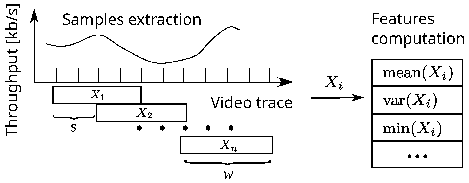
Figure 1. Identifying patterns within a univariate time series involves extracting features from sequential sliding windows of fixed length w = 4 and step size = 2 , where each window is represented as a vector in the form { X 1 , X 2 , , X n } . The distance between feature vectors is then calculated and used to identify feature clusters.
Electronics 14 03587 g001
Figure 2. Calculation steps of the filter approach: computation of mutual information coefficient for each feature (5), sorting the features according to their value by computing the Relevance Rank (6), and calculation of pairwise correlations between features (8).
Electronics 14 03587 g002
Figure 3. Weight update for a feature vector F i = { x , y } . With feature x’s decreasing dispersion measured with D i (12), its weight w x increases as in (13). The dispersion of feature y is higher than that of feature x; therefore, its weight decreases.
Electronics 14 03587 g003
Figure 4. The architecture of LassoNet consists of a residual layer, shown in blue, and multiple hidden layers, shown in green. The residual layer is subject to L1 regularisation, skipping selected elements of an input vector.
Electronics 14 03587 g004
Figure 5. Sample segments of the traffic traces utilised in the experiment: (a) YouTube set to 720p, (b) YouTube set to 1080p, (c) Amazon set to 720p, (d) Amazon set to 1080p, (e) Amazon set to 720p, (f) Amazon set to 1080p.
Electronics 14 03587 g005
Figure 6. Temporary characteristics of extracted features: moving average for (a) YouTube and (b) moving average for Amazon, variance for (c) YouTube and (d) Amazon. Window length w = 32 , step size s = 1 .
Electronics 14 03587 g006
Figure 7. Histogram of the variance for different window lengths w: (a) 16, (b) 32, and (c) 64.
Electronics 14 03587 g007
Figure 8. F1 score vs. number of features vs. method for a window length w = 32 , step size s = 1 and (a) 4, (b) 8, and (c) 16 features.
Electronics 14 03587 g008
Figure 9. F1 score as a function of (a) a sliding window length w for 8 features and the interval s = 1 , (b) an adaptive sliding window length w for 8 features and the interval s = 1 , and (c) an interval s between subsequent sliding windows for 8 features and the window length w = 32 .
Electronics 14 03587 g009
Table 1. Network throughput traces used in the experiments.
ActivityResolutionAverage (MB/s)Variance (MB/s)
YouTube720p0.320.45
1080p0.621.73
Netflix720p0.410.58
1080p0.610.69
Amazon720p0.410.20
1080p0.840.64
Table 2. F1 score, precision, and recall for feature selection methods for a window length w = 32 , step size s = 1 , and 8 features.
MethodMeasureVideo Trace
Youtube_720Youtube_1080Netflix_720Netflix_1080Amazon_720Amazon_1080
Filter:
mutual information
F1 score0.790.80.760.780.790.8
precision0.710.730.780.840.730.72
recall0.890.880.740.730.860.9
Filter:
Chi-Square test
F1 score0.770.780.720.740.770.78
precision0.690.710.760.780.710.71
recall0.860.860.690.70.850.86
Wrapper:
Weighted Kmeans
F1 score0.840.870.810.820.830.84
precision0.80.830.840.840.780.81
recall0.890.910.780.80.890.87
Wrapper:
Sequential Forward Selection
F1 score0.830.860.820.830.840.85
precision0.790.850.860.830.810.83
recall0.880.870.790.830.880.88
Embedded:
LassoNet
F1 score0.850.860.830.820.840.86
precision0.80.790.890.860.80.82
recall0.910.950.780.780.880.91
Autoencoder + SVMF1 score0.820.820.790.780.810.83
precision0.760.750.820.770.730.76
recall0.890.90.760.790.910.92
Table 3. Comparison of selected feature selection methods by relative execution time.
MethodRelative Exec. Time
Filter (MI)<1%
Wrapper (Weightened KMeans)≈62%
Embedded (LassoNet)≈38%
Disclaimer/Publisher’s Note: The statements, opinions and data contained in all publications are solely those of the individual author(s) and contributor(s) and not of MDPI and/or the editor(s). MDPI and/or the editor(s) disclaim responsibility for any injury to people or property resulting from any ideas, methods, instructions or products referred to in the content.