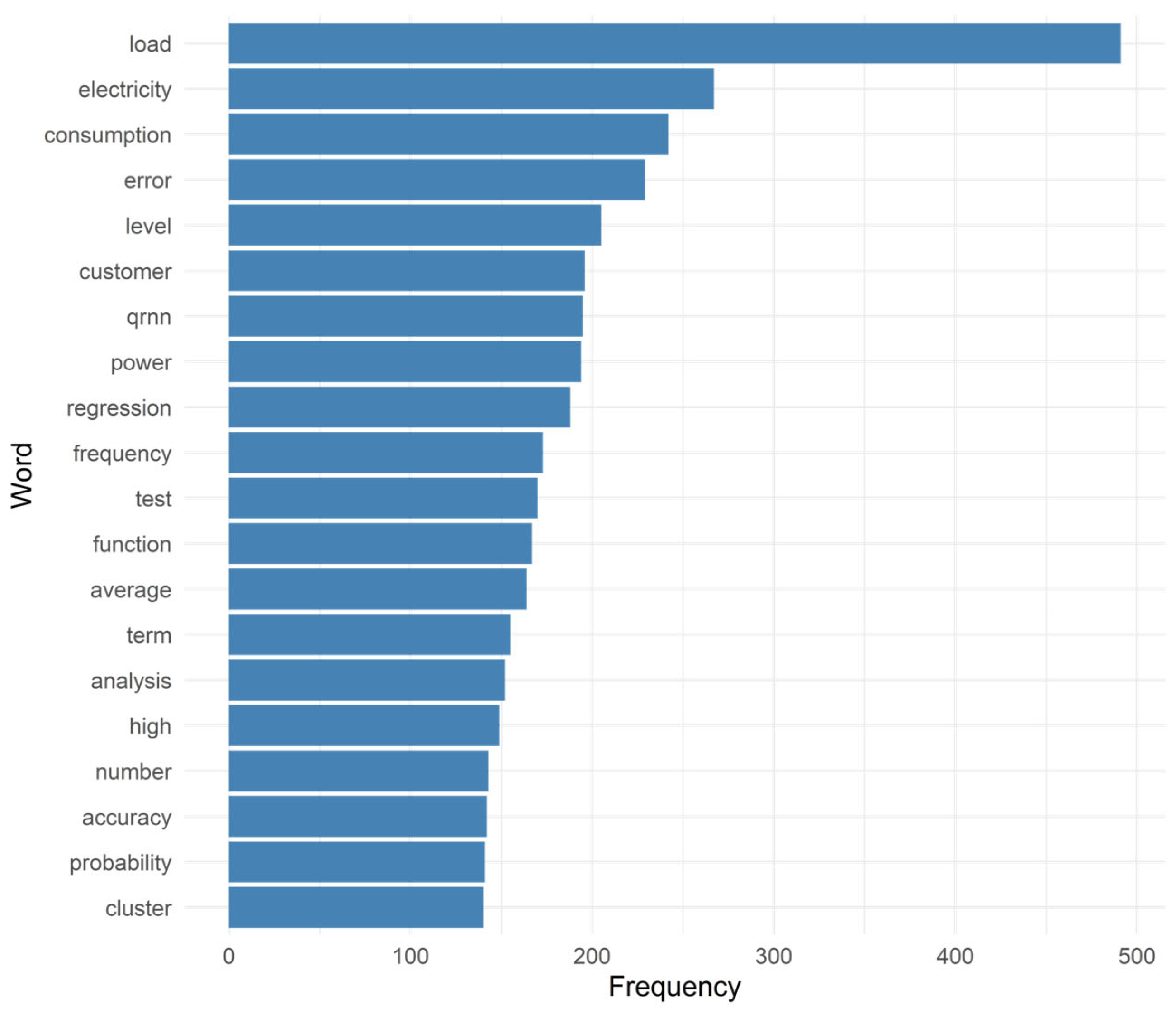
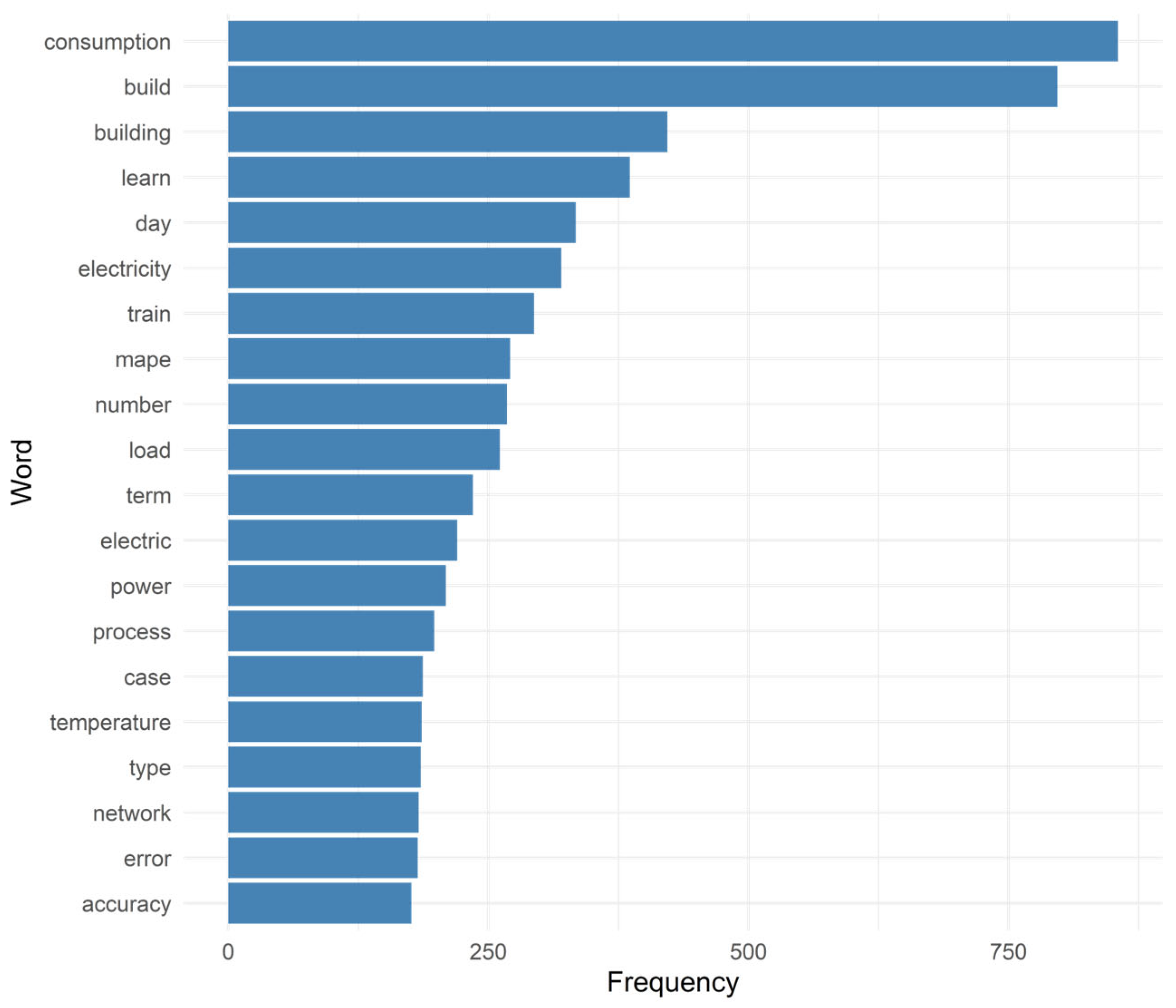
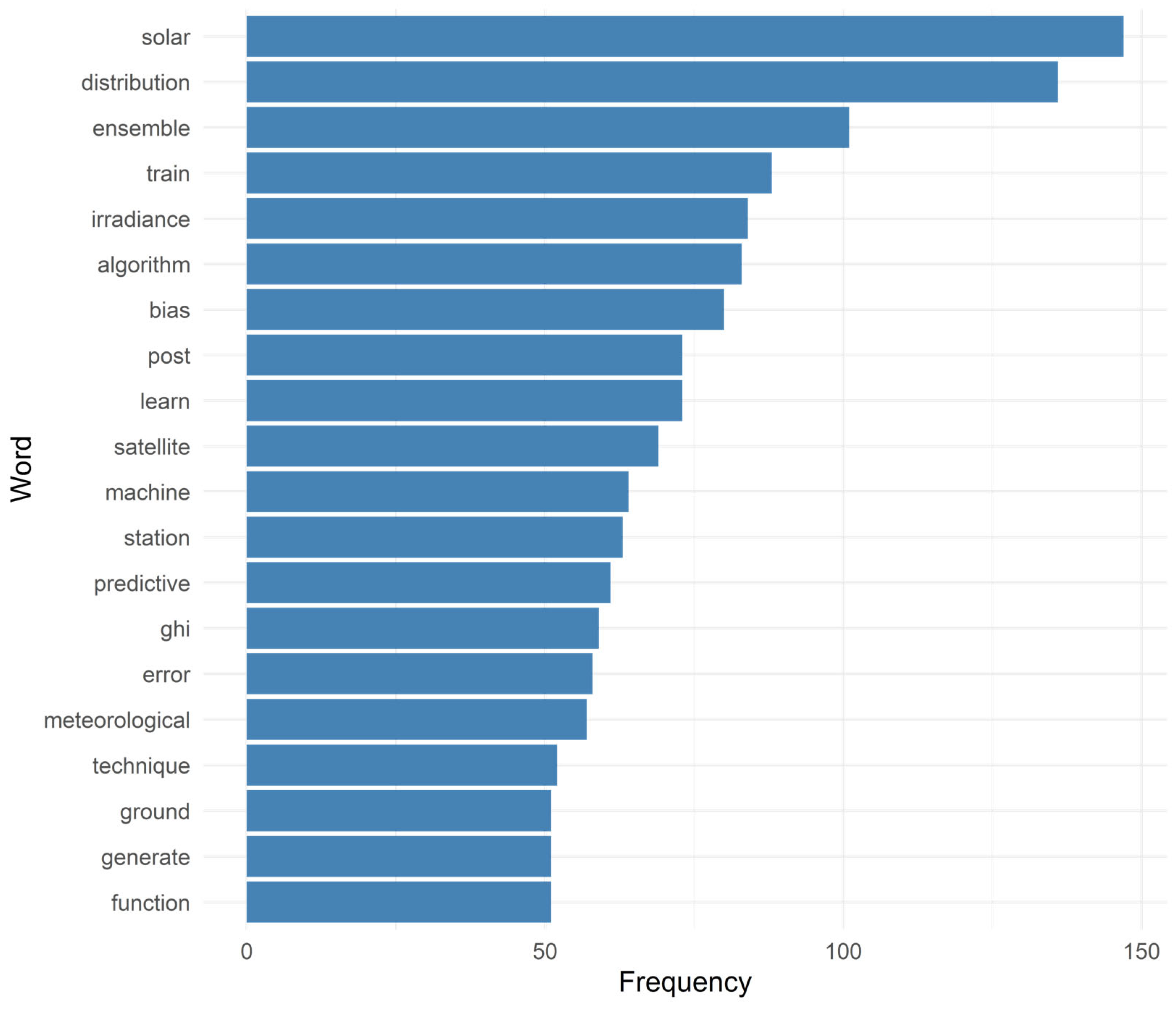
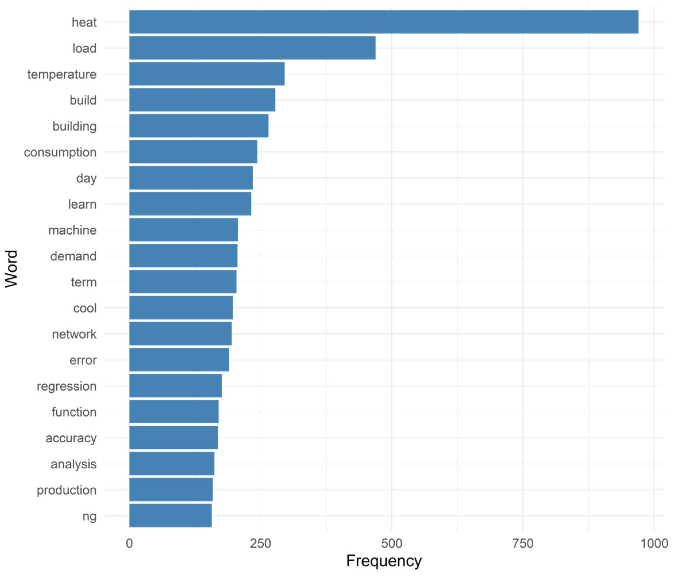
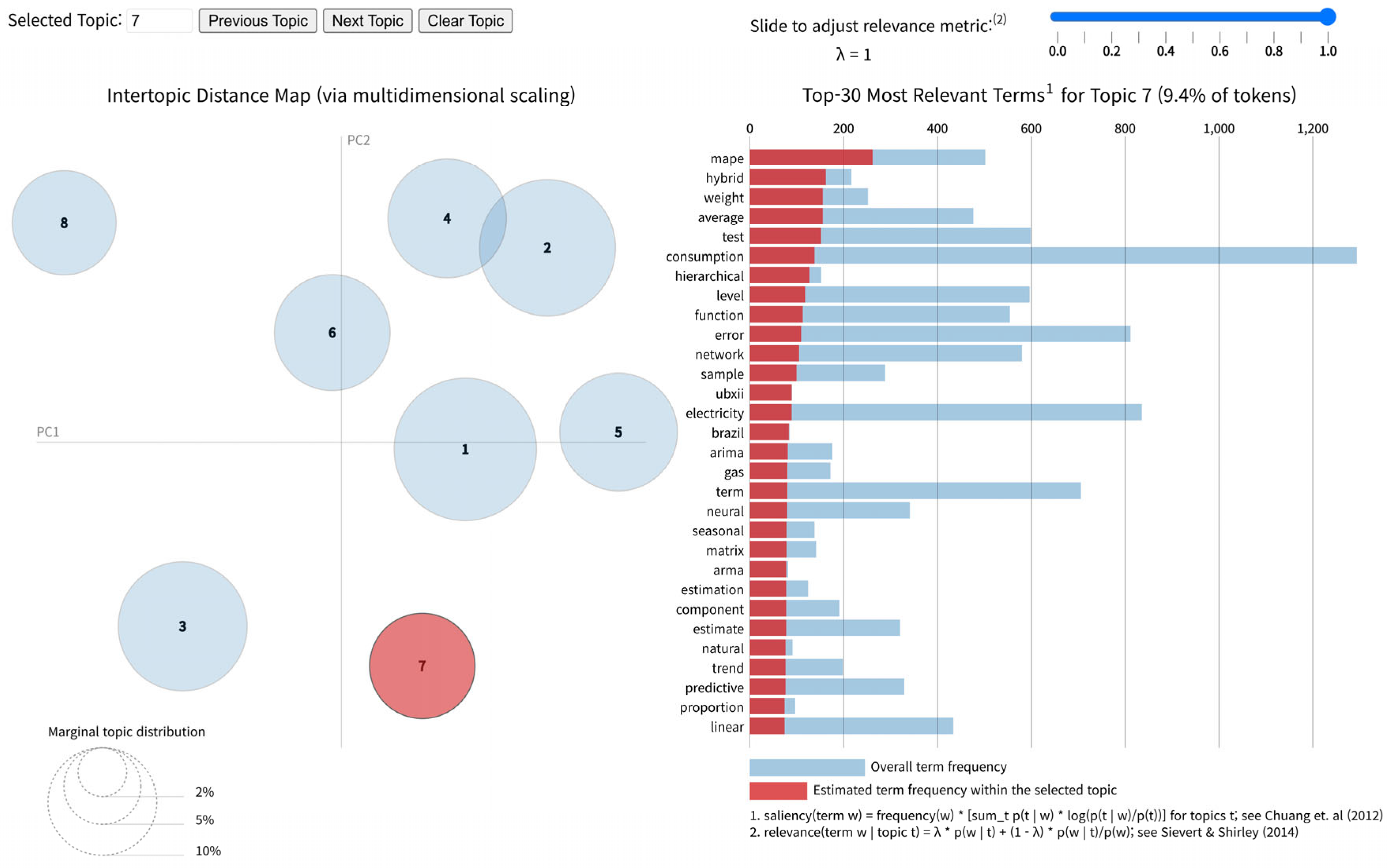
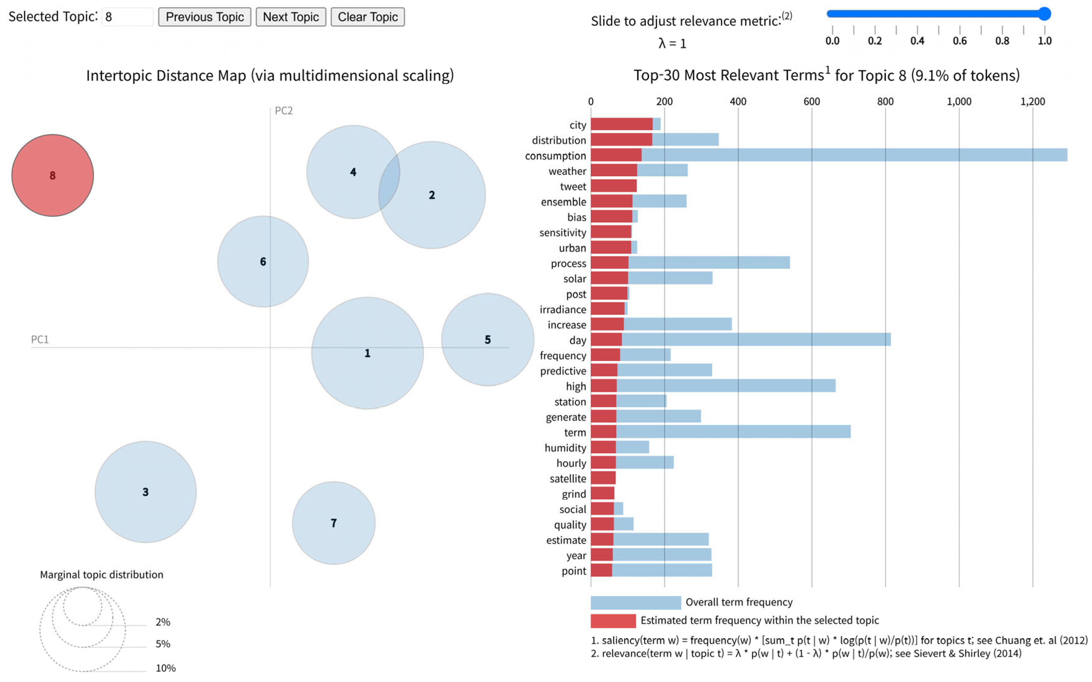
Within this study, we classified the literature into six overarching domains: electricity forecasting, energy forecasting in buildings, solar energy forecasting, wind energy forecasting, thermal and gas energy forecasting, and hybrid or emerging systems such as electric vehicles and energy storage. The studies within each domain were arranged chronologically, enabling readers to follow the progression of methodologies from earlier contributions to more recent advances. This organization provides a comprehensive overview across diverse energy sectors while also facilitates an understanding of the technological trends and research trajectories that have shaped the field over time.
2.4.1. Electricity Forecasting
Electricity consumption forecasting, which plays a fundamental role in ensuring grid stability, optimizing generation dispatch, managing market pricing, and minimizing outages, is one of the most mature and actively researched areas in energy analytics [
52]. Relative to other energy forecasting domains, electricity load prediction benefits from the abundance of historical data and relatively well-structured inputs, e.g., time-of-day indicators and weather variables. Yet, this apparent regularity belies significant challenges, especially in localized or sector-specific contexts, where nonlinearities and unexpected variations are introduced by behavioral, environmental, and technological factors.
Table 2 lists selected studies using R for electricity forecasting. It outlines dataset details, model types, performance results, and main R packages, highlighting recent trends across regions and time scales.
Recently, the R programming environment has been adopted extensively for electricity forecasting tasks across academic and applied settings. Its open-source ecosystem supports a wide range of modeling strategies, including classical time series methods, e.g., autoregressive integrated moving average (ARIMA) and exponential smoothing state space (ETS); tree-based learners, e.g., the random forest (RF) and gradient boosting methods; and advanced hybrid models that combine statistical baselines with ML or neural networks (NNs). Importantly, R’s support for hierarchical time series modeling, probabilistic forecasting, and explainable artificial intelligence (XAI) techniques closely aligns with the evolving demands of modern electricity systems.
During 2020, Gontijo and Costa [
53] employed hierarchical time series models in R to analyze Brazil’s hourly electricity generation across regions and energy sources. The dataset spanned wind, hydro, thermal, solar, and nuclear generation from 2018 to 2020, and forecasting was performed using the ARIMA and ETS models via the hts package. A comparison of reconciliation strategies included bottom-up, top-down, and minimum trace (MinT). MinT exhibited the highest accuracy with the lowest MAPE and RMSE values, demonstrating the benefits of optimal aggregation in national energy systems.
In 2021, Zhang and Li [
54] proposed a closed-loop clustering (CLC) framework for hierarchical load forecasting, in which clustering was iteratively linked with model fitness. Using real smart meter datasets from Ireland (January–November 2012) and incorporating South Wales PV and meteorological data, they implemented multiple linear regression (MLR) via the lm function in RStudio across all methods. Their findings demonstrated that the CLC framework consistently outperformed conventional approaches—including top-down, Gaussian mixture models (GMMs), ensemble, and bottom-up strategies—achieving MAPE reductions of 19.90%, 18.40%, 26.89%, and 52.20%, respectively.
Allee et al. [
55] used survey and smart meter data from 1378 customers across 14 rural Tanzanian mini-grids to predict initial electricity demand during the first year after connection. They trained least absolute shrinkage and selection operator (LASSO) and RF models and benchmarked them against an intercept-only baseline, evaluating performance through leave-one-group-out cross-validation at the site level. The best site-level result was obtained with LASSO (median absolute percent error of 37%), followed by RF (45%) and the intercept-only baseline (62%). At the customer level, the reported median absolute error was 66%. All analyses were conducted in R (RStudio) using ggplot2, dplyr, glmnet, randomForest, and Boruta for feature screening.
By 2022, Silva et al. [
56] conducted a comparative study of statistical and NN models for monthly electricity consumption in the Brazilian industrial sector using data from the Central Bank of Brazil. The series was split into January 1979–December 2018 for model fitting and January 2019–December 2020 for forecasting. The authors evaluated Holt–Winters, seasonal ARIMA (SARIMA), dynamic linear model, and TBATS (short for Trigonometric seasonality, Box–Cox transformation, ARMA errors, Trend, and Seasonal components), alongside neural network autoregression (NNAR) and multilayer perceptron (MLP). All statistical analyses and graphics were performed in R, with implementations referencing the forecast package for time series models, including TBATS and the dlm package for dynamic linear model (DLM). Across horizons, the MLP achieved the best overall performance, and it recorded MAPE = 1.48 (fit) and 3.41 (forecast), outperforming the remaining candidates on average.
Subsequently, in 2023, Zhou et al. [
57] proposed D-MCQRNN (short for deep learning-based monotone composite quantile regression neural network), a deep learning (DL) architecture that combines dropout and DropConnect regularization in a monotone composite quantile regression NN. Here, the model was trained on hourly electricity load and meteorological data from Henan Province, China, and it was evaluated in terms of the continuous ranked probability score (CRPS), coverage ratio, and volumetric efficiency. The architecture was implemented using the keras and tensorflow packages in R and outperformed several benchmarks, including quantile RF (QRF), Bayesian NNs, and least-squares support vector machine (SVM) benchmarks. The D-MCQRNN model obtained up to 26.76% improvement in the CRPS.
Later, in 2024, Cabreira et al. [
58] employed a hierarchical structure comprising national, regional, and state levels to forecast monthly electricity consumption in Brazil’s industrial sector. Their dataset, which was obtained from Brazil’s Energy Research Company (EPE), spanned from 2004 to 2022, offering long-term, disaggregated consumption records. Moreover, the forecasting models included ETS, ARIMA, feedforward NNs (FFNNs), and long short-term memory (LSTM) networks. The bottom-up LSTM model yielded the best performance among the hierarchical reconciliation strategies, which consisted of bottom-up, top-down, and optimal combination methods, achieving an MAPE of 2.35% and an RMSE of 433.36 GWh. The analysis employed several R packages, including the hts, fpp3, and forecast packages, and highlighted the effectiveness of disaggregated modeling in capturing localized consumption dynamics.
Ribeiro et al. [
59] proposed the unit Burr XII quantile ARMA (UBXII-ARMA) model to forecast proportions bounded between 0 and 1, e.g., stored hydroelectric energy. The model, which was developed in R, combines quantile regression with the autoregressive moving average (ARMA) structure, a logit link, and harmonic seasonal covariates. Validated on Brazilian hydropower data (2000–2019), the UBXII-ARMA model outperformed the beta-ARMA and Kumaraswamy ARMA (KARMA) models in terms of the MAPE while also detecting structural breaks that other models overlooked.
Abbasabadi and Ashayeri [
60] proposed the TwEn ML framework to predict hourly electricity demand in urban areas using social media activity. The dataset used in the study included geotagged tweets aligned with the New York Independent System Operator (NYISO)’s electricity demand data for 2021. The features included tweet frequency per borough and hour, which was extracted using the academictwitteR package. The implemented models included artificial NN (ANN), decision tree (DT), RF, and gradient boosting machine (GBM) models, which were evaluated using the caret, randomForest, and nnet packages. The ANN models yielded R
2 values between 0.72 and 0.99 depending on the season, revealing strong correlations between digital social rhythms and energy consumption.
He et al. [
61] designed the hybrid MIDAS-NAMEMD-QRNN model for the mixed-frequency probabilistic forecasting of peak electricity demand. In the study, the data were sourced from Vermont and Houston, incorporating hourly load, daily weather, and policy variables. The R implementation used mixed data sampling (MIDAS) for frequency alignment, noise-assisted multivariate empirical mode decomposition (NAMEMD) for signal decomposition, and a quantile regression NN (QRNN) for quantile estimation. Kernel density estimation (KDE) translated the outputs into full probability distributions. The model achieved MAPE values of 1.19% and 1.86% for Vermont and Houston, respectively, as well as CRPS reductions relative to nine baseline models.
Mutombo et al. [
62] forecast the total electricity generation in South Africa using multidecade data from the International Energy Agency covering 1990–2020. The energy sources included coal, nuclear, hydro, biofuels, oil, wind, solar PV, and solar thermal. In addition, multiple regression models were tested using R, with model m06 (comprising coal, nuclear, and solar PV) achieving the best performance (R
2 = 0.9988, RMSE = 807.66). The lm and ggplot2 packages were used alongside diagnostics for multicollinearity, heteroscedasticity, and outliers.
Most recently, in 2025, Zournatzidou [
63] modeled renewable energy consumption using six R-based ML models, i.e., the RF, support vector regression (SVR), extreme gradient boosting (XGBoost), light GBM (LightGBM), LASSO, and MLP models. In addition, a novel predictor, the energy uncertainty index, was introduced. The LightGBM model produced the most accurate 6-month forecast (MAPE = 1.15%), followed by XGBoost. Rolling-window cross-validation and log-differencing ensured stationarity and model robustness, demonstrating the effectiveness of boosting techniques in volatile energy markets.
Keka and Cxicxo [
64] compared linear and nonlinear approaches for electric load analysis using R. They assembled 15-min load data and 30-min weather data from three substations of an anonymized utility (Electrical Company Z, Region X) and aggregated them to 30-min intervals covering July 2009 to July 2014. The models included linear regression, MLR, polynomial regressions of degrees 2–4, and an interaction specification. Drawing on analysis of variance (ANOVA), Akaike information criterion (AIC), and Bayesian information criterion (BIC) comparisons, the degree-4 polynomial provided the lowest AIC/BIC values, with an adjusted R-squared of 0.07619 and an F-statistic of 279. The implementation was conducted in R (e.g., stats::lm()), with standard visualizations used to examine distributional patterns.
Short-term load forecasting (STLF) models are prone to overfitting when high-frequency sensor data and numerous engineered covariates are added without controls for parsimony [
65]. Heterogeneous data sources—such as supervisory control and data acquisition (SCADA), surveys, and social media activity—can introduce target leakage and misaligned timestamps, inflating reported accuracy; strict temporal separation and careful lag design are therefore essential [
66]. In multi-level planning, forecasts developed independently at feeder, regional, and national scales may not aggregate consistently. When a hierarchy exists, reconciliation methods such as the MinT framework offer a practical solution [
67]. For sites with limited local history, such as EV charging stations or new buildings, generalization often suffers; transfer learning and low-data strategies can mitigate this limitation [
68]. These patterns recur across the reviewed electricity studies and frequently employ ensembles with hierarchical tools in R.
2.4.2. Energy Forecasting in Buildings
Forecasting energy consumption in buildings is a crucial yet complex task within the energy analytics landscape. Unlike grid-level electricity demand, which is influenced by large-scale consumption trends and macroeconomic factors, building-level forecasting must capture localized dynamics, e.g., occupancy behavior, heating, ventilation, and air conditioning (HVAC) operation, thermal inertia, equipment schedules, and microclimatic variation. The diversity of building types, ranging from residential apartments and offices to commercial hotels and healthcare facilities, adds a layer of complexity since each class exhibits distinct temporal and structural energy patterns.
The growing availability of high-resolution building data, frequently derived from smart meters and environmental sensors, has expanded the possibilities for developing granular forecasting models, and this trend aligns well with the capabilities of the R programming environment, which offers extensive support for time series modeling, statistical learning, and model interpretability. R has been employed across a wide spectrum of applications, including STLF, daily peak demand estimation, and integrated modeling of internal conditions, e.g., temperature, humidity, and lighting levels. Moreover, energy forecasting in buildings frequently incorporates transfer-learning strategies, hybrid ensemble frameworks, and online learning algorithms, each of which benefits from R’s flexibility and modularity.
Table 3 provides a summary of representative studies that applied R for forecasting energy use in buildings, based on the information available in the original papers.
During 2020, Shen et al. [
69] investigated how psychological and behavioral factors affected household electricity usage through a behaviorally informed SVR model. In this case, data were collected via surveys and smart meters in Hangzhou, China, including 48 variables ranging from appliance ownership and occupancy patterns to personality traits based on the Big Five model. Using AIC, 18 predictors were retained. The SVR model with a radial basis function kernel was optimized using a genetic algorithm (GA) in R, achieving an adjusted R
2 value of 0.6857. Implemented with the GA, e1071, and custom SVR packages, the model forecasted household consumption and simulated reductions under targeted interventions, exhibiting up to 12.1% energy savings.
Dominguez-Jimenez et al. [
70] examined seasonality in EV charging demand using aggregated load data from 44 public charging stations in Boulder, Colorado, spanning 1 January 2018 to 28 February 2019. Preprocessing, modeling, and evaluation were carried out in RStudio (Version 1.1.442). For regression analysis, RF and a quasi-Poisson generalized linear model (GLM) were compared; RF generally provided higher accuracy, although quasi-Poisson captured large demand variations more effectively. For classification, twelve algorithms were tested, and GLMNET (short for LASSO and elastic-net regularized GLMs) was ultimately identified as the best-performing model. The abstract reported test accuracy as high as 100%, while the main results indicated an average test accuracy of approximately 98.78%. Cross-validation summaries also highlighted XGBoost as achieving the highest mean accuracy and AUC among the classifiers considered.
Additionally, Zor et al. [
71] evaluated two symbolic regression models, i.e., gene expression programming (GEP) and group method of data handling (GMDH), to forecast short-term electricity consumption in a large hospital in the Eastern Mediterranean, Turkey. Both models were constructed in R without prior feature selection using one year of data, including meteorological and calendar variables. The GEP model generated an interpretable equation using four inputs, and the GMDH model employed seven variables and higher-order polynomials, achieving slightly better accuracy (MAPE = 0.620% vs. 0.641%). In addition, a temporal error analysis revealed challenges during holidays and seasonal changes, emphasizing the need for flexible modeling approaches.
Moon et al. [
72] addressed the cold-start problem in STLF, where a lack of historical data makes accurate prediction difficult. They introduced SPROUT (short for solving the cold-start problem in STLF using tree-based methods), which is a hybrid model implemented in R that combines two RF approaches, i.e., one trained on only 24 h of data from the target building and another trained on data from 14 other buildings. Beyond this, a transfer-learning mechanism was employed to identify the most similar building based on the load patterns using the Euclidean distance. The final forecast combined the outputs from both models and adjusted for different calendar variables, e.g., weekdays and holidays. SPROUT significantly outperformed 14 benchmark models in multistep hourly forecasts, exhibiting improvements in terms of the MAPE, RMSE, and mean absolute error (MAE) metrics.
Fan et al. [
73] proposed a transfer-learning methodology for 24 h-ahead building energy prediction using the Building Data Genome dataset (507 nonresidential buildings, primarily in America and Europe), with one year of hourly data per building. Of these, 407 buildings formed the source domain and 100 the target domain (83,060 vs. 19,027 samples after windowing). All preprocessing and modeling were conducted in R using the keras package. The pre-trained network stacked two one-dimensional convolutional layers (kernel = 4; filters = 200 and 100) with a bidirectional LSTM and embeddings for categorical inputs, outputting the next 24 h load. In the source domain, the pre-trained model achieved an RMSE of 10.97 kW, compared with 16.58 kW and 14.39 kW for previous-day and previous-week benchmarks, respectively. For transfer to target buildings, two strategies were tested: feature extraction (Model A) and weight initialization (Model B). Under Scenario A (random 20–80% of a year), mean performance improvement ratios (PIRs) reached 0.490–0.483 at 20%, with benefits diminishing as data volume increased. Under Scenario B (2–10 months), mean PIRs ranged from 0.729 to 0.779 for feature extraction and 0.676 to 0.752 for weight initialization, indicating an average error reduction of at least 67%.
In 2021, Wenninger and Wiethe [
74] benchmarked five R-based ML models, i.e., ANN, SVR, RF, XGBoost, and D-vine copula quantile regression (QR) models, for residential heating energy prediction in Germany. All models were trained on data from 25,000 residential buildings and validated against 345 energy performance certificate (EPC)-certified samples. They found that all models outperformed the engineering-based EPC benchmark. XGBoost obtained the best performance with a coefficient of variation of 0.329, compared to 0.614 for the EPC model. Importantly, feature importance analysis identified living area, insulation, and energy source as primary predictors.
By 2022, Fan et al. [
75] introduced a conditional variational autoencoder (CVAE)-based data augmentation method to improve STLF in buildings with limited data. Implemented in R, the CVAE model employed 7-day historical consumption and seasonal variables to generate synthetic training data. In this study, two CVAE architectures were tested, one with fully connected layers and another with one-dimensional convolutional layers. Moreover, enhanced artificial NNs (ANNs) incorporating one-dimensional convolutional NN (CNN) and bidirectional LSTM (BiLSTM) layers were trained on data from 52 buildings in the Building Data Genome Project with and without augmentation. The augmented models showed a 12–18% improvement in coefficient of variation of the root mean square error (CVRMSE), outperforming traditional methods, e.g., Gaussian noise injection. The study demonstrated R’s utility in data preprocessing, generative modeling, and model evaluation.
Jozi et al. [
76] proposed a contextual learning framework implemented in R to enhance the short-term energy consumption, generation, room occupancy, brightness, and temperature predictions in smart buildings. This method clusters historical data using k-means based on contextual features, e.g., ambient temperature, lighting, and occupancy. Within each cluster, various models, including SVM, hybrid neural fuzzy inference system (HyFIS), Wang–Mendel, and GFS.FR.MOGUL (short for genetic fuzzy system for fuzzy rule learning based on the MOGUL methodology) models, were trained. The system was deployed in real-time at the Research Group on Intelligent Engineering and Computing for Advanced Innovation and Development (GECAD) Building N in Portugal and integrated 15-min sensor data into a building energy management system. It improved the forecast accuracy compared with LSTM baselines and enabled automated control suggestions for HVAC and lighting systems.
Kim et al. [
77] developed a multi-level stacked regression framework to predict 15-min-ahead electricity consumption in a steel hot rolling mill (HRM). At Level 0, the framework incorporated linear regression, RF, GBM, and SVM, whose out-of-fold predictions were subsequently combined via ridge regression at Levels 1 and 2. ARIMA and ARIMA with exogenous variables (ARIMAX) models served as benchmarks. The study was conducted in R 3.6.3 and RStudio 1.3, using plant operation records aggregated into 15-min intervals from 1 January 2019 to 30 January 2020. Across multiple time-ordered train/test splits, the stacked ridge meta-model (RG2) demonstrated the highest predictive accuracy, achieving an MAPE of approximately 7.4–8.2% for +15-min forecasts, and outperforming both manual operator estimates and individual baseline models.
Moon et al. [
78] developed the ranger-based online learning approach (RABOLA) model for robust STLF in buildings with dynamic consumption patterns. In the first stage, they trained several ensemble models, i.e., RF, GBM, and XGBoost, on historical data. Their predictions, along with time-based (hour, weekday, and holiday) and environmental (temperature and humidity) features, were then used as inputs in the second stage, where an online RF model was implemented using the ranger package in R, updated via a 7-day sliding window. Using hourly data from two office buildings in Washington, USA, RABOLA achieved strong performance (MAPE = 11.03%, CVRMSE = 18.68%), outperforming DL models, e.g., gated recurrent unit and attention-based LSTM models. Feature importance and partial dependence plots (PDPs) enhanced interpretability.
Subsequently, in 2023, Kondi-Akara et al. [
79] analyzed daily per-capita electricity consumption for twelve West and Central African cities using a nonstationary MLR framework in which both the base load and weather sensitivities varied over time. Key predictors included cooling degree days, a humidity index, and wind speed. Their results indicated that temperature explained approximately 25–70% of the day-to-day variability in electricity demand, with each 1 °C increase associated with a 3–4% rise in base consumption in coastal cities such as Mindelo and Dakar, and a 6–10% rise in most Sahelian and tropical cities. Importantly, humidity effects reached up to 70% of the temperature effect in several Sahelian and tropical locations, underscoring the importance of nonstationary demand dynamics.
Later, in 2024, Zhang et al. [
80] developed a forecasting framework for high-rise hotel energy use in Guangzhou, China, by combining EnergyPlus simulation outputs with ML. They defined six prototype hotel configurations based on 78 architectural layouts, simulated 5000 buildings using Latin hypercube sampling, and identified key predictors through standardized regression coefficients. In this study, 15 R-based models were evaluated, with quadratic polynomial regression demonstrating the highest accuracy and stability (R
2 > 0.95, error range = 2.38–8.11%). In the study, all analyses were conducted in R, demonstrating its effectiveness for high-resolution forecasting in the hospitality sector.
Most recently, in 2025, Cebeci and Zor [
81] examined the impact of COVID-19 on electricity demand at a university hospital using deep polynomial NNs (DPNNs) and GEP. Their dataset included 15-min electricity usage, meteorological variables, and pandemic indicators, e.g., case counts and restriction levels. The DPNN model achieved superior normalized RMSE (5.66% hour-ahead and 11.13% day-ahead) and was five times faster than the GEP model. It is worth noting that both models were developed in R, highlighting the importance of integrating public health variables in high-resolution energy forecasting.
Timur and Üstünel [
82] considered hourly electricity consumption forecasting for a 24/7 industrial facility in Adana, Turkey. Their dataset integrated over 30,000 observations of SCADA-based energy readings and Modern-Era Retrospective Analysis for Research and Applications version 2 (MERRA-2) meteorological variables, e.g., temperature and humidity. Additionally, they tested five forecasting models, i.e., MLR, GMDH, MLP, gradient-boosted decision tree (GBDT), and GEP models. Preprocessing and modeling were performed in R using the dplyr and caret packages, as well as custom scripts. The GBDT model obtained the most accurate results with an MAPE of 0.827%, indicating its strength in high-dimensional, nonlinear applications.
At the building scale, models often overfit when numerous occupancy, HVAC, and microclimate variables are applied to short historical records [
83]. Regime shifts—such as holidays, retrofits, or maintenance—disrupt stationarity and degrade performance; online (RABOLA) and transfer-learning (SPROUT) approaches consistently stabilize forecasts under such conditions [
84]. Small-sample facilities face additional challenges from data sparsity and missing values; data augmentation methods such as CVAE-based generation and robust imputation provide interim solutions until sufficient data are collected [
85]. Where simulation tools are available, integrating physics-based models (e.g., EnergyPlus-based hybrid forecasting) with ML enhances extrapolation and reduces the brittleness of purely statistical approaches [
86]. Equally important, contextual and smart-building frameworks and pandemic-sensitive modeling highlight the importance of adapting to behavioral and external disruptions. Taken together, these strategies improve forecast stability without compromising interpretability in the building-scale studies reviewed here.
2.4.3. Solar Energy Forecasting
Although benefiting from relatively regular diurnal and seasonal cycles, solar energy forecasting presents its own set of challenges due to the influence of weather variability, cloud cover, and the spatial heterogeneity of irradiance levels. The integration of distributed solar PVs into modern power systems requires forecasts that are both accurate and adaptable across multiple scales, from rooftop systems to utility-scale solar farms. In contrast to demand-side energy forecasting, which is frequently dependent on behavioral and economic signals, solar forecasting is intrinsically dependent on environmental and atmospheric conditions, thus rendering meteorological modeling an essential component of the task.
Against this backdrop, the reviewed studies demonstrate how R has been employed to develop diverse solar forecasting models, including ML-based approaches to predict solar irradiance and PV output, time series techniques for clear-sky index (CSI) forecasting, and postprocessing frameworks for probabilistic output generation. Some studies incorporated satellite-derived or ground-based weather observations, and others utilized clustering methods or ensemble learners to enhance predictive stability under varying sky conditions. This methodological diversity reflects the multifaceted nature of solar forecasting and highlights R’s adaptability in supporting the development, evaluation, and deployment of exploratory models.
Table 4 presents key R-based approaches for forecasting solar energy across various studies.
During 2020, Yagli et al. [
87] evaluated the feasibility of using bias-corrected satellite-derived global horizontal irradiance (GHI) as the sole input for univariate ML forecasts. Using data from 15 Baseline Surface Radiation Network (BSRN) stations, several models, including the Cubist, generalized linear model via penalized maximum likelihood, SVM, RF, and projection pursuit regression models, were trained using R’s caret package. Moreover, kernel conditional density correction enabled comparable accuracy between satellite-based and ground-based forecasts, supporting scalable approaches in sensor-limited regions.
Yagli et al. [
88] developed a probabilistic forecasting framework that combined 20 ML and time series models to predict the CSI. Implemented using data from the U.S. SURFRAD (short for Surface Radiation Budget) network, the forecasts were postprocessed via generalized additive models (GAMs) for location, scale, and shape (GAMLSS) and QRFs. GAMLSS allowed for detailed modeling of the distributional properties, and the QRF offered nonparametric flexibility. Both methods improved the CRPS considerably, with a skill score gain of up to 58.12% over climatological baselines.
Dobreva et al. [
89] presented a comprehensive evaluation framework for PV performance forecast models that combined graphical residual analysis with two scale-independent metrics (s and mm). Using monthly outputs from two grid-connected systems in Namibia—NamPower 1 (p-Si, 63.455 kW) and Güldenboden (CdTe, 15.660 kW)—they developed four PVSYST variants (NP1X, NP1Y, GnX, and GnY) and assessed them in RStudio. Across both qualitative and quantitative comparisons, NP1Y (with shading correction) delivered the best performance, while GnX was the least accurate. For example, NP1Y achieved s = 0.467 and mm = 0.957 under the proposed evaluation metrics. The dataset consisted of AC energy records extracted from the SMA (short for System-, Mess- and Anlagentechnik) Sunny Portal, covering September 2012–July 2017 (59 months) for NamPower 1 and August 2014–December 2018 for Güldenboden, with the 2018 records flagged, leaving 41 reliable months.
In 2021, de Freitas Viscondi and Alves-Souza [
90] compared SVM, artificial NNs (ANNs), and extreme learning machines (ELMs) for daily solar irradiance prediction in São Paulo, Brazil, using the IAG-USP (short for Institute of Astronomy, Geophysics, and Atmospheric Sciences of the University of São Paulo) meteorological dataset (final modeling set: 19,359 daily records, 1962–2014). Data ingestion, model training, and evaluation were conducted in RStudio with the e1071, neuralnet, and ELMR packages. The dataset was shuffled, normalized, and divided into 15,000 training and 4358 testing instances, and model performance was assessed using MAE, RMSE, and Pearson’s correlation coefficient. Among the parameter-group experiments, SVM produced the lowest RMSE, whereas ELM trained substantially faster. The best SVM configuration (SVM_4) achieved MAE = 2.05 MJ/m
2 and RMSE = 2.78 MJ/m
2 with r = 0.89, while the best ELM setup (ELM_4) delivered MAE = 2.35 MJ/m
2 and RMSE = 3.09 MJ/m
2, with training approximately 94% faster than SVM.
By 2022, Mukilan et al. [
91] presented a rooftop-level PV forecasting method using restricted Boltzmann machines (RBMs) implemented in R. The study addressed environmental nonstationarity by applying a data pipeline involving cleaning, scaling, and k-fold cross-validation. The RBM models outperformed ANNs and backpropagation NNs in terms of MAPE and F-measure, reaching up to 99% accuracy. While sensitive to initialization, the RBM models demonstrated a strong capacity for capturing nonlinear dependencies.
Most recently, in 2024, Masache et al. [
92] compared decision tree-based approaches—RF and its quantile hybrid QRRF (short for quantile regression RF)—with a quantile generalized additive model (QGAM) for short-term GHI forecasting. The dataset consisted of hourly GHI observations collected between March 2017 and June 2019 at the NUST (short for Namibia University of Science and Technology) radiometric station in Windhoek, Namibia. Missing values were imputed using Hmisc, hierarchical interactions were selected with hermit, and the models were implemented in R 4.3.2 (randomForest, quantregForest, mgcViz; simulations via JWileymisc). In simulation experiments, QGAM outperformed QRRF on pinball loss and mean absolute scaled error (MASE). For the Windhoek case study, QGAM produced the lowest RMSE (21.233) and CRPS (205.39), whereas QRRF achieved the lowest MAE (11.11), MASE (0.1177), and pinball loss (5.555). A Diebold–Mariano test (
p = 0.2943) suggested that the overall predictive accuracy of QGAM and QRRF did not differ significantly.
Forecast accuracy declines under rapid cloud dynamics and in areas without dense ground-sensor coverage [
93]. Two effective strategies include (1) applying weather-regime classification before modeling and (2) using bias-corrected satellite GHI where local measurements are unavailable [
94,
95]. Another persistent drawback is poor uncertainty calibration, where point forecasts conceal operational risk; probabilistic post-processing methods such as GAMLSS and QRF improve CRPS and enhance decision-making utility [
96]. Model choice (e.g., SVM vs. ELM) also can influence robustness under long historical datasets. Seasonal imbalances, particularly in winter and autumn, can shift feature importance [
97]; rule-based or hybrid learners and neural approaches for rooftop PV often demonstrate greater robustness across seasons.
2.4.4. Wind Energy Forecasting
Wind energy production forecasting presents distinct challenges due to the inherently volatile and geographically variable nature of wind. For instance, wind speeds are highly sensitive to short-term meteorological fluctuations, terrain complexity, and elevation, unlike solar irradiance, which typically exhibits predictable diurnal and seasonal patterns. This variability reduces the accuracy of the output predictions and introduces operational risks for grid integration and scheduling, particularly in regions with renewable energy portfolios that are heavily reliant on wind power. Wind forecasting models must incorporate both temporal and spatial dynamics across various forecasting horizons to address these challenges.
In this domain, the R programming environment supports a broad spectrum of methods, including classical time series approaches and advanced ML and ensemble techniques. Many previous studies have employed autoregressive models, e.g., the ARIMA and SARIMA models, for short-term forecasting because of their transparency and interpretability. Yet, other studies have employed ML models, e.g., RF and SVM models, to capture the nonlinear relationships and interactions among meteorological variables. Moreover, hybrid or hierarchical structures are being adopted increasingly to support multiscale forecasting and temporal reconciliation.
Table 5 presents key R-based approaches for forecasting wind energy across various studies.
During 2020, Zhang et al. [
98] investigated the resilience of wind forecasting models against false data injection attacks (FDIAs). Implemented in R and RStudio using Monte Carlo simulations, the study compared three deterministic models, i.e., multiple nonlinear regression (MNR), ANN, and SVM models, and three probabilistic models, i.e., QR, QRNN, and k-nearest neighbors (KNN) with kernel density estimation (KNN-KDE) models, on the GEFCom2014 dataset. The SVM and KNN-KDE model demonstrated the highest resistance against data corruption, maintaining lower RMSE values and quantile loss under increasing attack severity. However, all models collapsed under full-scale FDIAs, highlighting the urgent need for cybersecurity-aware designs in forecasting architectures.
In 2021, Costa et al. [
99] introduced the analog-based dynamic time scan forecasting (DTSF) model for multistep wind speed prediction. The DTSF model matches the current observations with historical sequences using polynomial similarity functions and extrapolates future values accordingly. An ensemble version, referred to as eDTSF, aggregates forecasts from multiple analogs to enhance robustness. Validated on 241,200 wind speed observations from Bahia, Brazil, the DTSF model outperformed 11 benchmark models across several error metrics. Implemented in R via the custom DTScanF package, the study demonstrates R’s ability to support high-resolution, analog-based forecasting frameworks.
Most recently, in 2024, Prieto-Herráez et al. [
100] developed the two-stage ensemble optimization for load operations (EOLO) wind forecasting system for integration into Spain’s electricity market. Developed entirely in R, EOLO first minimizes prediction error using an ensemble of eight ML models. It subsequently adjusts the forecasts to optimize the economic returns. Leveraging meteorological data, market pricing, and historical production records, EOLO achieved an average prediction error of less than 8% and increased profitability by up to 2% in selected wind farms. The system is also scalable and requires no manual configuration when applied to different sites, thereby making it suitable for operational deployment.
English and Abolghasemi [
101] proposed a hierarchical wind forecasting framework that reconciles predictions across temporal resolutions ranging from 5 min to 1 h. Then, linear regression models were constructed at each temporal level using R’s hts package and reconciled using bottom-up, top-down, and MinT methods. The results of empirical evaluations confirmed that the integrated hierarchical model outperformed the separately trained approaches for each resolution. These findings underscore the importance of temporal consistency and highlights the strengths of R in hierarchical forecasting applications.
Wind forecasting studies often contend with data sparsity—such as limited mast measurements or coarse reanalysis grids—and terrain-induced nonstationarity, both of which degrade the performance of classical ARIMA and SARIMA baselines [
102]. Under these conditions, analog and ensemble approaches (e.g., DTSF and eDTSF) as well as tree-based learners have shown more robust gains [
103]. Multi-horizon forecasting can introduce temporal inconsistencies when 5-min, 15-min, and hourly models are trained separately; hierarchical reconciliation methods (e.g., MinT) restore cross-resolution coherence [
104]. More recently, a critical issue has emerged in the form of adversarial or corrupted telemetry, such as false data injection attacks (FDIAs), where several models fail catastrophically under severe tampering; robust preprocessing and quantile-based learners have demonstrated stronger resilience in testing [
105].
2.4.5. Thermal and Gas Energy Forecasting
Accurate forecasting of thermal energy demand is a critical task for cities and utilities pursuing decarbonization and efficiency in heating systems. In contrast to electricity forecasting, which frequently targets immediate load fluctuations, the prediction of thermal demand and natural gas consumption must address slower, behavior-driven dynamics that are influenced by various factors, e.g., building insulation, occupancy patterns, climatic conditions, and heating system design. Taken together, these factors interact across seasonal and diurnal cycles, creating modeling challenges that require both physical and data-driven insights.
Recent investigations using the R programming environment have highlighted a wide spectrum of modeling strategies tailored to thermal and gas applications, encompassing linear regression to estimate transmission and infiltration losses, ML approaches (e.g., ANN and SVR models) to capture short-term and seasonal patterns, and hybrid frameworks integrating physically simulated data with empirical modeling techniques. R’s flexibility in supporting diverse analytical pipelines has made it an effective tool for fine-grained, building-level prediction and broader district heating and natural gas load forecasting.
Table 6 presents key R-based approaches for forecasting thermal energy across various studies.
During 2020, Liu et al. [
106] proposed a hybrid prediction model for hourly district heating load based on association rule mining and SVR. In this study, two feature selection techniques were evaluated, i.e., one based on the Spearman correlation coefficient and the other using the Eclat algorithm to extract frequent itemsets, both of which were implemented in RStudio. The Eclat-based SVR (E-SVR) model outperformed its Spearman-based (S-SVR) counterpart, reducing the RMSE value by 28.1% and improving accuracy by 8.2%. The historical water supply temperature was the most significant predictor. The study highlights R’s ability to combine unsupervised feature selection with supervised ML techniques for thermal energy analytics.
Bujalski and Madejski [
107] forecasted combined heat and power (CHP) heat production in the heating season (November–March) using a GAM with weather inputs (air temperature, solar irradiation, and wind speed) and hour of day, calibrated adaptively with a 12-day moving window. With the inclusion of irradiation and wind (Model M1) improved accuracy, particularly in March. Across the season, the average MAPE was below 7%, with monthly MAPE between ~5.2% and 7.5%, and RMSE reductions were observed when solar effects were incorporated.
In 2021, Li and Yao [
108] designed a hybrid framework that integrates EnergyPlus-based physical simulations with ML to predict heating and cooling demand across 442 buildings in Chongqing, China. In the study, energy use intensity values simulated via the Urban Modeling Interface were employed to train 10 ML models, including SVR with linear, polynomial, and Gaussian kernels; RF; XGBoost; ANN; ordinary least squares; ridge regression; LASSO; and elastic net models, all of which were implemented using R’s
caret package. At the individual building level, the polynomial SVR model achieved the highest accuracy, and the Gaussian SVR model performed best in terms of aggregated demand predictions. The data-driven models provided over 1000-fold speed improvements compared with simulation runs, thereby enabling rapid assessment of retrofit scenarios.
Dulce-Chamorro and Martínez-de-Pisón [
109] developed parsimonious predictive models of hospital cooling energy demand for San Pedro Hospital in Logroño, Spain, using building management system (BMS) data. The measurements were aggregated on an hourly basis, missing values were interpolated, thermal power and energy were derived, and the target variable (ENERGYKWHPOST) was smoothed with a Gaussian filter (window = 11). The final feature set included calendar indicators and temperature-related variables. Two modeling stages were carried out: the first used data from January 2017–February 2018 for training and March 2018–February 2019 (even/odd weeks) for validation and testing, while the second followed system optimizations introduced around April 2018. Models were optimized with GAparsimony in R, focusing on SVR with RBF kernel, ANN, and XGBoost. SVR delivered the best single-model performance with three features in the initial round, and an ensemble of SVR, ANN, and XGBoost further improved RMSE compared to the best individual model.
Żymełka and Szega [
110] developed a short-term heat demand prediction model for gas-fired CHP systems equipped with thermal storage. Using a feedforward ANN with five hidden layers, implemented entirely in R, the model used the ambient temperature, wind speed, humidity, and previous 24 h heat demand as inputs. Trained on hourly data from the heating season using a 70–15–15 data split, the ANN significantly outperformed an exponential regression benchmark, achieving RMSE, R
2, and MAPE values of 7.18, 0.9886, and 3.65%, respectively. The findings of the study highlight the feasibility of R-based ANN models for accurate thermal load forecasting in complex energy infrastructures.
By 2022, Shin and Cho [
111] developed and evaluated machine learning models to predict the coefficient of performance (COP) of an air-cooled heat-pump system using operational data collected in a university laboratory. The input variables included heat-source and load-side inlet and outlet temperatures, heat-pump power, and indoor and outdoor air temperatures, all measured at one-minute intervals. The dataset was divided into 70% training (5124 samples) and 30% testing (2196 samples), and the models were implemented in RStudio 1.2.1335. Four algorithms were compared—ANN, SVM, RF, and KNN. Among them, ANN achieved a mean bias error (MBE) of −3.6 and a CVRMSE of 5.4% (error range: −7.8–9%), thereby meeting ASHRAE (short for American Society of Heating, Refrigerating and Air-Conditioning Engineers) Guideline 14 criteria. Results for SVM, RF, and KNN were also summarized for comparison. Ultimately, the ANN model was deployed in the building automation system (BAS) to enable real-time performance monitoring.
Subsequently, in 2023, Pala [
112] proposed a multihybrid long-term forecasting framework for monthly natural gas consumption in the U.S. vehicle fuel and industrial sectors. Using the forecastHybrid package in R, six models, i.e., auto.arima, nnetar, stlm, thetam, ets, and tbats, were combined under equal-weighted (EW), variable-weighted, and cross-validated weighting (CVW) schemes. The CVW ensemble yielded the best results for the industrial dataset (MAPE = 3.19%), whereas the EW ensemble yielded the best results for the vehicle fuel data (MAPE = 5.40%). The results indicated that the ensembles of statistical and neural models outperformed the standalone DL models, e.g., the MLP and ELM models, particularly for highly seasonal and nonlinear time series.
Bujalski et al. [
113] modeled day-ahead district-heating load in the off-season (June–August) using a generalized additive mixed model (GAMM)—a GAM extended with an autoregressive error term—and a 14-day sliding training window, incorporating calendar-pattern smooths. This configuration eliminated residual autocorrelation and achieved the highest test accuracy. The best-performing variant (AR order ≈ 1–3) yielded an RMSE of 0.84 MW and an MAPE of 3.26% for an average load of ~21 MW, with monthly MAPE ranging from 2.7% to 3.9% (lowest in July). Ambient temperature contributed minimally during the transitional months, making calendar effects the dominant predictors.
Most recently, in 2025, Tudor et al. [
114] developed an ML-based analytical framework to assess and forecast fossil fuel reliance across the EU-27, modeling the share of fossil fuels in the final energy consumption using an RF regressor. This model incorporated six predictors, i.e., gross domestic product (GDP), population, industrial production, CO
2 emissions, share of renewable energy, and energy intensity, and it was implemented in R using the randomForest, caret, iml, and pdp packages. The performance of the model was evaluated using leave-one-out cross-validation with interpretability enhanced via Shapley additive explanations (SHAP) values and PDPs. The results projected a reduction in fossil fuel share from 1.8% in 2022 to 1.33% by 2030, aligning with the EU Green Deal targets and illustrating the efficacy of interpretable ensemble learning under constrained data conditions.
Thermal demand patterns are affected by shoulder-season regime shifts and occupant behavior, which many models fail to capture [
115]. For instance, incorporating irradiation and wind improved accuracy during transitional months, whereas calendar-pattern smooths and autoregressive terms stabilized forecasts in off-season periods. Applying seasonal filtering and change-point detection can improve stability during these transitional periods [
116].
Smart meter data streams are frequently noisy or incomplete, making thorough cleaning and imputation essential before any model comparison [
117]. Hospital-scale studies highlighted the importance of handling missing values, while association-rule mining extracts robust predictors. Combining simulation outputs with ML enables generalization to climates or retrofit conditions beyond those observed in the training data integrating EnergyPlus simulations with ML. Moreover, interpretability can be maintained through association-rule mining and SHAP/PDP analyses help system operators trust the results [
118].
At the broader district heating network (DHN) level, aggregated models can mask infrastructure heterogeneity; segment-specific approaches revealed fine-grained variation and avoided bias from averaging. Ensemble strategies for long-term gas consumption further illustrate the importance of flexible modeling. These findings confirm that R-based pipelines effectively balance accuracy, stability, and interpretability in thermal and gas demand forecasting [
119].
2.4.6. Hybrid and Emerging Energy Systems
Beyond conventional energy domains, specialized forecasting tasks that fall outside the boundaries of single-source or sector-specific energy modeling have been investigated. Such tasks encompass predicting stored hydropower levels, simulating energy usage during public health crises, forecasting battery behavior in UPS systems, predicting EV charging demand, and assessing building-level micro-grid dynamics. Although diverse in scope, these studies share a methodological emphasis on adapting traditional forecasting frameworks to accommodate irregular data structures and domain-specific constraints.
The versatility of the R programming environment and its modular package ecosystem makes it particularly effective for addressing such unconventional forecasting challenges. For instance, whether estimating bounded time series, integrating clustered regressors into ARIMA, modeling behavioral features in electric mobility, or transferring shared structures across charging stations with Gaussian processes, R offers robust support through customizable model architectures, diagnostic tools, and user-friendly visualization. The ability to model novel problem settings flexibly is crucial as energy systems become increasingly interconnected and policy-relevant, particularly for analysts working at the intersection of energy, climate, and society.
Table 7 summarizes representative models and key innovations in hybrid and unconventional energy forecasting studies.
During 2020, Haider et al. [
120] proposed a cluster-assisted ARIMA framework for forecasting battery voltage in data-center UPS systems, in which cluster members were incorporated as external regressors in the ARIMA model. The dataset was obtained from a large-scale social media company in China and contained one year of one-minute measurements (470,226 records) across 40 VRLA batteries. During the observation period, four discharge cycles and three power surges were recorded. Clustering was performed on a monthly basis using k-shape and DTW. When inconsistency among cluster members was detected, the relevant members were passed as external regressors (xreg) to ARIMA, implemented with the forecast package, while clustering was executed using dtwclust. Across batteries and performance metrics (RMSE, MAE, MAPE), the k-shape-clustered ARIMA (CK) improved accuracy compared with both single-battery and total predictors, and also outperformed the DTW-clustered ARIMA (CDTW).
Almaghrebi et al. [
121] focused on session-level electricity demand forecasting for plug-in electric vehicle charging events. Here, the dataset included more than 22,000 real-world charging sessions collected over seven years from public stations in Nebraska. Each session’s input features included charging history statistics, session timing, pricing policy, and user behavior. Subsequently, R was used to implement and compare linear regression, support vector machine (SVM), RF (via ranger), and XGBoost models with tuning via the caret package. The XGBoost mode achieved the best RMSE and R
2 values of 6.68 kWh and 51.9%, which were further improved when outlier sessions were removed. The findings of the study confirmed the predictive value of behavioral features in electric mobility applications.
Vink et al. [
122] analyzed a building-scale micro-grid in Tsukuba, Japan, to assess the one-year forecasting potential of solar PV generation and building electricity demand. They applied linear, nonlinear, and SVR approaches, finding that PV output was linearly related to solar irradiance, whereas purchased electricity (demand) followed a quadratic relation with temperature. For PV, SVR improved RMSE in 2015–2016, whereas linear regression performed better in 2017. For demand, the quadratic model consistently outperformed the linear specification. The combined models estimated electricity costs within approximately 8% of actual values.
In 2021, Gilanifar and Parvania [
123] proposed a clustered multinode learning model with Gaussian processes (GPs) to predict flexible energy demand across multiple EV charging stations. Their dataset, which was gathered from 53 charging stations in Utah, included daily load curves and limited metadata per station. The model employed
k-means clustering to identify similar stations and transferred shared structure via linear predictors while considering residual uncertainty with GPs. Implemented in R, the clustered multi-node learning with Gaussian process (CMNL-GP) method improved the RMSE by over 30% in low-data scenarios compared with the ARIMA and NN baseline models.
Taken together, these studies illustrate how modular, open-source tools can be combined to explore novel forecasting frontiers—whether addressing geospatial heterogeneity, data sparsity, or the integration of domain-external variables (e.g., clustered battery data or EV charging sessions). Accordingly, this domain serves as a proving ground to extend R’s capabilities beyond traditional energy forecasting paradigms, encouraging innovation in modeling practices and systems-level understanding. Each application area (e.g., UPS batteries, EV charging, or micro-grids) presents unique modeling challenges, ranging from high temporal variability and spatial heterogeneity to long-term policy sensitivity and data limitations, and these studies demonstrate how R’s extensive package ecosystem, transparency, and flexibility support a wide spectrum of analytical requirements.
Yet, research in this area contends with heterogeneous, irregular data—such as clustered or incomplete charging sessions—and nonstandard metrics, all of which complicate benchmarking [
124]. Studies showed more stable performance across varying regimes [
125]. Given the novelty of these tasks, transparent preprocessing and reproducible workflows are as important as raw accuracy for ensuring reusability [
126]. Ultimately, R emerges not only as a statistical programming language but as a comprehensive platform that can be utilized to develop interpretable, adaptable, and context-sensitive energy forecasting models.
