Article

Multi-Feature Fusion YOLO Approach for Fault Detection and Location of Train Running Section

1
School of Traffic & Transportation Engineering, Central South University, Changsha 410075, China
2
Key Laboratory of Traffic Safety on Track, Ministry of Education, School of Traffic & Transportation Engineering, Central South University, Changsha 410075, China
3
China Railway Siyuan Survey and Design Group Co., Ltd., Wuhan 430063, China
4
School of Mechanical Science and Engineering, Huazhong University of Science and Technology, Wuhan 430074, China
*
Author to whom correspondence should be addressed.
These authors contributed equally to this work.
Electronics 2025, 14(17), 3430; https://doi.org/10.3390/electronics14173430
Submission received: 30 June 2025 / Revised: 4 August 2025 / Accepted: 7 August 2025 / Published: 28 August 2025

Abstract

This paper investigates the implementation of the YOLO (You Only Look Once) framework for defect detection, specifically targeting challenging conditions such as low-light environments, occluded objects, and requirements for non-contact measurement. Empirical evaluations demonstrate that the YOLO architecture delivers exceptional object detection capabilities, enabling rapid yet precise real-time analysis, scalability across diverse object sizes, and resilience to environmental variability. By integrating a multi-scale feature fusion strategy, the framework significantly enhances the detection accuracy of defective components. Furthermore, its non-invasive approach eliminates potential damage risks and operational costs associated with conventional inspection methodologies. Experimental results on a 1270-image dataset show 87.5% mAP, 92% recall, 89% accuracy, and 22 FPS, demonstrating high performance.

1. Introduction

In the context of railway transportation and industrial production, the occurrence of defects is inevitable, particularly in critical components such as railway fasteners, welded joints, and track surfaces. These encompass welding imperfections (e.g., cracks, pores), material defects (e.g., surface scratches, fatigue cracks), and fastener looseness—all of which pose significant risks to operational safety [1,2,3]. For example, loose fasteners in railway tracks can lead to rail misalignment and derailment accidents, while undetected welding defects may cause structural failures in train components [4]. Figure 1 shows a schematic diagram of fastener loosening defects and surface defects of the product material.
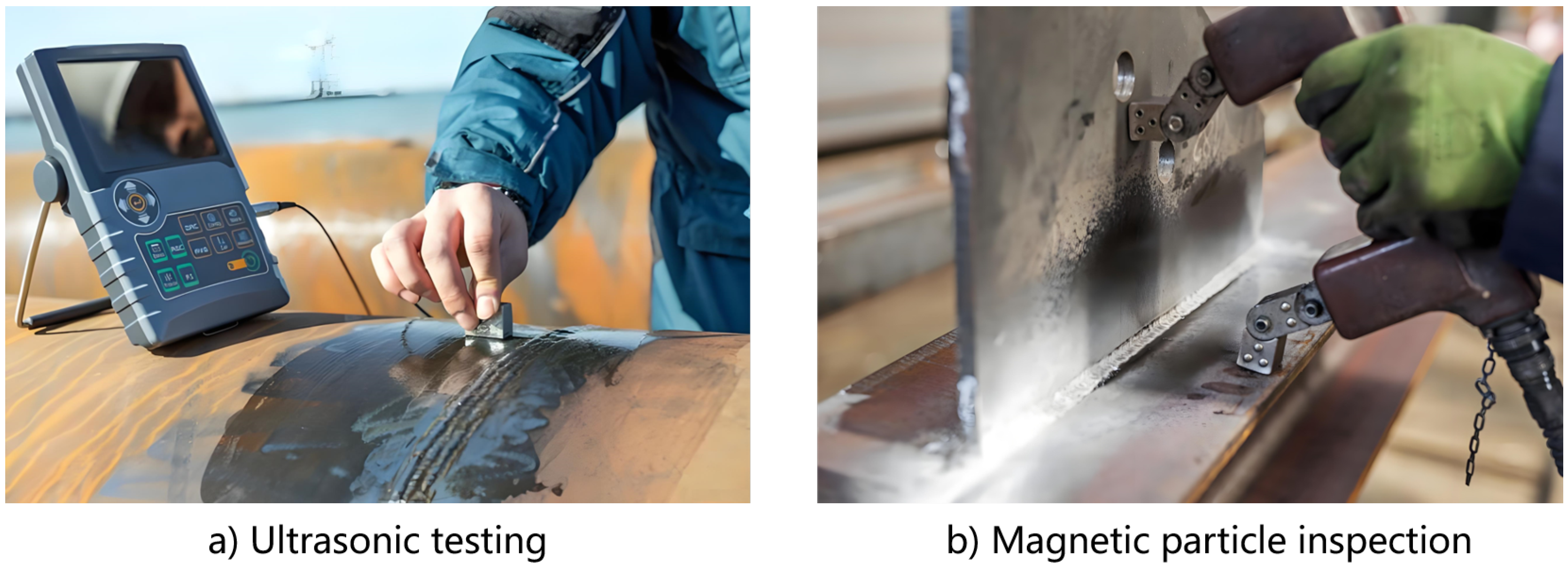
Defects in industrial products, whether they are microscopic cracks in precision components, misalignments in assembly parts, or anomalies in electronic circuit boards, can trigger a cascade of consequences, from product recalls and production downtime to catastrophic safety incidents. For example, in the aerospace industry, a minute surface flaw in a turbine blade can lead to fatigue failure under high-stress conditions, potentially endangering flight safety and causing significant economic losses. In the automotive manufacturing sector, defective welding joints in vehicle frames may compromise structural integrity, leading to serious accidents and substantial brand-image damage. Consequently, research on defect detection is of paramount importance. Currently, the methodologies used most frequently for defect detection include ultrasonic testing, magnetic particle inspection, optical machine vision inspection, and visual examination, among others. As shown Figure 2, ultrasonic testing and magnetic particle inspection are conducted.
Each of the aforementioned methods carries its unique set of advantages and disadvantages. Ultrasonic testing and magnetic particle testing necessitate considerable operational experience [5] from the personnel involved, and they also impose certain limitations on the materials of the products being tested [6]. Furthermore, visual inspection is prone to significant errors. Given these considerations, this article introduces a detection method that leverages machine vision [7]. Following the marking of fasteners according to assembly specifications, as illustrated in the accompanying Figure 3, images of the marked areas are systematically acquired on a regular basis. A deep learning detection algorithm, grounded in YOLO-v3 [8], is utilized to detect the marked areas and evaluate the marks. When the displacement of the mark exceeds the predefined safety threshold, it is concluded that the fastener has loosened and requires repair. The implementation process of the method is shown in Figure 4. The core workflow involves:
  • Marker-based Fastener Monitoring: Applying standardized markings to critical components (e.g., fasteners) according to assembly specifications, enabling systematic visual tracking of displacement anomalies.
  • Multi-scale Feature Fusion: Utilizing YOLO-v3’s hierarchical feature pyramid network (FPN) [9] to detect defects across varying scales, from micro-cracks to macro-looseness, ensuring robustness against lighting variations and partial occlusions.
  • Non-contact Image Analysis: Eliminating physical contact with inspected objects, thereby reducing damage risks and operational costs while maintaining high detection precision.
This method has been experimentally validated to achieve high accuracy. By combining traditional marking techniques with advanced YOLO-v3-based deep learning detection algorithms, intelligent detection of fastener looseness has been achieved. By regularly collecting images of the marked areas and conducting detection, this method can monitor the looseness of fasteners in real time and issue timely warnings when potential problems are discovered, improving the timeliness and accuracy of detection. Compared with traditional contact detection methods, this method adopts non-contact image acquisition and detection methods, avoiding errors or damage caused by contact and improving the reliability and safety of detection. The equipment required for this method is simple, easy to install and maintain, and the detection process is relatively simple and clear, making it easy to operate and manage.

2. Related Work

2.1. Object Detection

Object detection, crucial in computer vision, plays a pivotal role in industrial applications such as quality control, production line automation, and equipment fault diagnosis. Traditional image algorithms and deep learning-based detection methods are commonly utilized for this purpose.
Among them, traditional image algorithms traverse the pixel values of the image, analyzing features such as grayscale value, variance, color, shape, contour, area, etc., to detect defects [10]. Template matching, a traditional algorithm, compares a predefined template with a test image to detect defects or targets. It excels in scenarios with regular shapes and stable backgrounds but struggles with complex or irregularly shaped objects. Traditional image algorithms are computationally efficient and advantageous for high real-time performance scenarios [11]. However, they are limited in detecting complex defects due to reliance on manual features and classifiers, and are sensitive to lighting variations and product/line changes [12].
Another algorithm leverages deep learning, employing a multi-layer neural network to automatically extract and classify image features through extensive data training. This approach obviates the need for manual feature extraction and exhibits superior generalization and adaptability. Some classic methods include the Convolutional Neural Network (CNN), a prevalent algorithm for image classification and recognition which automatically extracts and classifies image features through convolutional, pooling, and fully connected layers, and is frequently used for tasks like product defect detection and object identification. Another prevalent algorithm is the object detection series, exemplified by YOLO (You Only Look Once) and SSD (Single Shot MultiBox Detector). These CNN-based algorithms employ structures such as anchor boxes or Region Proposal Networks (RPNs) for precise localization and recognition of targets in images. Deep learning algorithms demonstrate robustness to lighting and noise, enhancing practical accuracy and reliability. However, they require extensive annotated data and impose significant computational and hardware demands. Therefore, in some scenarios that require high real-time performance, deep learning algorithms may need to be optimized and accelerated.
In this work, due to dim scene lighting, complex image backgrounds, and certain requirements for algorithm speed, the YOLO algorithm was chosen to achieve the final detection task. The next section will provide a detailed introduction to the YOLO algorithm.

2.2. YOLOs

The YOLOs (You Only Look Once series algorithm) stand as a pioneering single-stage object detection algorithm. Unlike two-stage methods that require extensive proposals and bounding-box generation and filtering, YOLOs integrate detection and classification through a single neural network, utilizing a global loss function, which reduces computational load, ensures real-time performance, and enables multi-scale detection. As an end-to-end system with a simplified network structure, YOLOs facilitate ease of implementation, optimization, and attain high accuracy. Since its inception, the YOLO algorithm has undergone multiple iterations from YOLO-v1 to YOLO-v5, with each update bringing significant improvements in architecture, principles, performance, and application scenarios. YOLO-v1 is the first to treat object detection as a regression problem, directly outputting the coordinates, confidence, and class probabilities of bounding boxes through CNN. YOLO-v1 uses 7 × 7 grid division to input images, with each grid responsible for predicting two bounding-boxes and one category label. Although its detection performance for small and overlapping objects is limited, its speed and background false detection rate are impressive. YOLO-v2 (also known as YOLO-9000) has made multiple improvements based on YOLO-v1, introducing batch normalization, anchor boxes, dimensional clustering, multi-scale training and testing, etc, which significantly improved the accuracy and speed of detection, and achieved detection of over 9000 categories. YOLO-v3 further improves the accuracy and speed of detection by using a deeper feature extractor Darknet-53 and an FPN (Feature Pyramid Network), supporting multi-label detection and capable of detecting objects at multiple scales [13]. YOLO-v3 also uses logistic regression instead of soft-max to predict class probabilities, allowing the model to handle multi-label problems more flexibly. Recent studies have applied YOLO-v3 to detect railway anomalies such as rail surface defects and overhead contact line faults, validating its potential in transportation infrastructure monitoring [14,15]. YOLO-v4 [16] introduces more latest object detection technologies based on YOLO-v3, such as a stronger feature extractor CSPDarknet53, which significantly improve the accuracy and speed of the model. YOLO-v4 has also improved its detection performance for small objects. Although the model structure is complex, it still achieves high efficiency and simplicity overall. YOLO-v5 [17] is a project developed by the community, which uses the PyTorch (https://github.com/ultralytics/yolov5/tags accessed on 6 August 2025) framework to implement the YOLO model and has made some improvements, such as using lighter feature extractors and simpler data augmentation, optimization methods, and detection techniques. YOLO-v5 performs well in both accuracy and speed, with a smaller model that requires less computing resources and is easy to use and deploy.
Overall, the YOLOs are constantly evolving in terms of speed, accuracy, and model size to meet the needs of different scenarios. Both the initial exploration of YOLO-v1 and the latest achievements of YOLO-v5 demonstrate the strength and broad application prospects of the YOLOs in the field of object detection. Taking into account various factors such as algorithm detection speed, accuracy, and computational cost, this work adopts the YOLO-v3 algorithm for defect detection. The implementation details will be introduced in detail in subsequent chapters.

3. Method

Due to the cluttered background of defect images, poor lighting conditions, and occlusion of target defects in this work, it is a relatively complex object detection task [18]. At the same time, in order to ensure industrial production efficiency, it is necessary to improve detection efficiency on the basis of ensuring detection accuracy [19]. In the YOLOs, YOLO-v3 introduces the FPN, which can fuse feature maps at different scales to achieve multi-scale object detection. At the same time, multi-scale prior anchors are used to greatly improve the prediction accuracy of bounding boxes, making YOLO-v3 perform very well in both detection accuracy and speed [20]. Therefore, YOLO-v3 is chosen to implement the detection task in this paper. This section will provide a detailed introduction to the algorithm.

3.1. The Overall Architecture of YOLO-v3

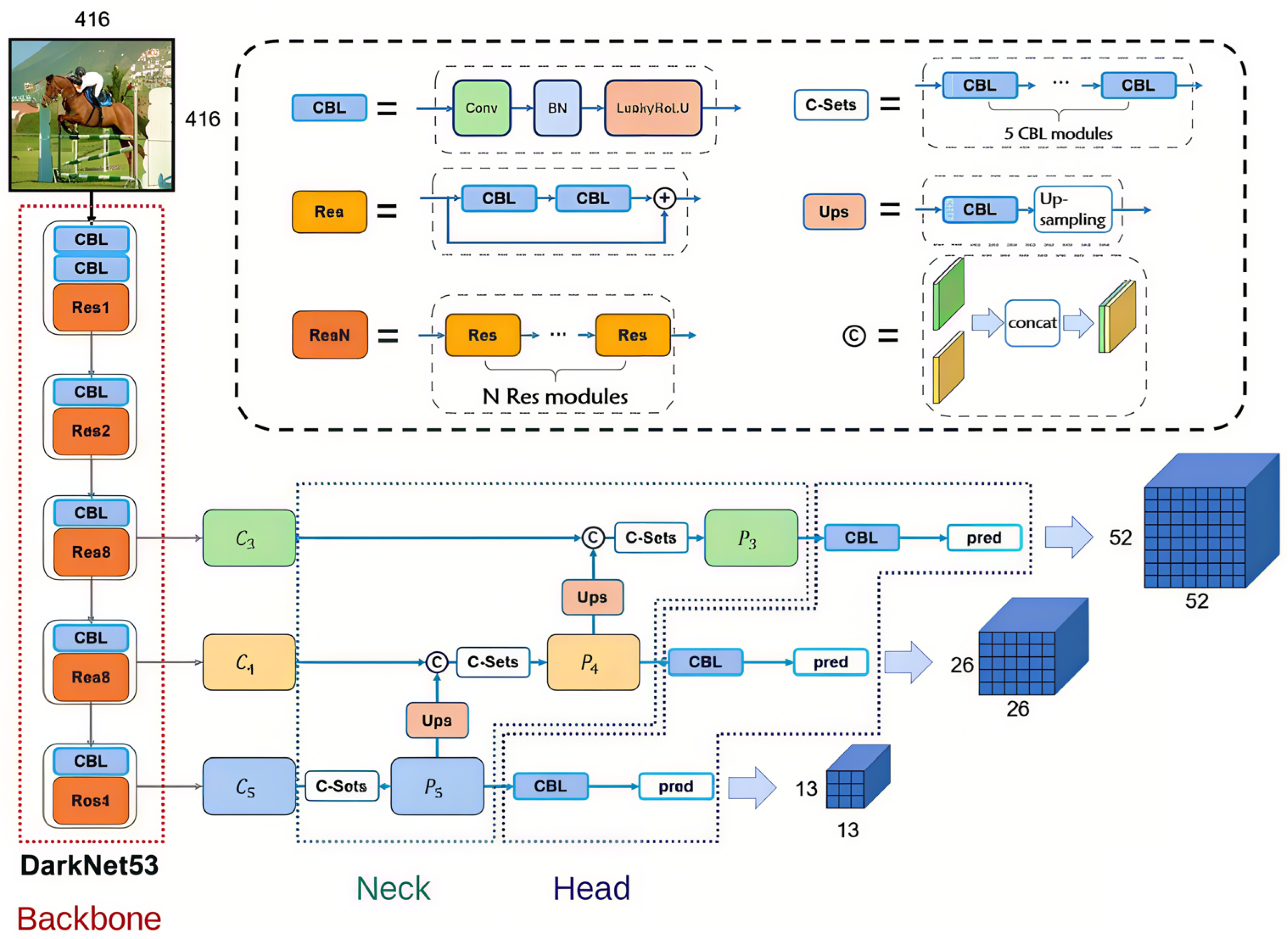
The algorithm architecture of YOLO-v3 mainly consists of three parts: feature extraction network (Backbone), feature fusion network (Neck), and detection head (Head). The overall architecture diagram of the YOLO-v3 network is shown in Figure 5. Among them, Backbone is used to extract high-level features of images, providing rich feature information for subsequent feature fusion and detection heads. Neck is responsible for fusing feature maps of different scales to improve their expressive power, which helps the network better adapt to targets of different sizes. More useful information is captured through upsampling and concatenation operations to improve the accuracy and recall of object detection. The Head part detects the position and category of the target based on the fused feature map, predicts the coordinates, confidence score, and category probability of the bounding box, and provides key information for the final target detection result.
The implementation process of YOLO-v3 algorithm is as follows:
  • Image input: Input an image of appropriate size and perform data augmentation operations such as random cropping, rotation, flipping, etc. to increase the robustness of the model.
  • Feature extraction: Use Darknet-53 backbone network to extract image features and generate multi-scale feature maps. These feature maps contain information of different scales and levels in the image.
  • Feature Fusion: FPN fuses feature maps from different scales to generate a feature pyramid with rich semantic information. This step helps the model better detect targets of different sizes.
  • Object detection: Apply convolutional and predictive layers on the feature pyramid to predict bounding boxes and category probabilities for each grid cell. YOLO-v3 adopts a multi-scale prediction strategy, which outputs feature maps of different sizes at different network layers to adapt to object detection of different sizes.
  • Post-processing: Apply Non-Maximum Suppression (NMS) to remove redundant bounding boxes and generate the final detection result. NMS compares the confidence levels of adjacent bounding boxes, retains the bounding box with the highest confidence level, and removes other bounding boxes with excessive overlap.

3.1.1. Backbone

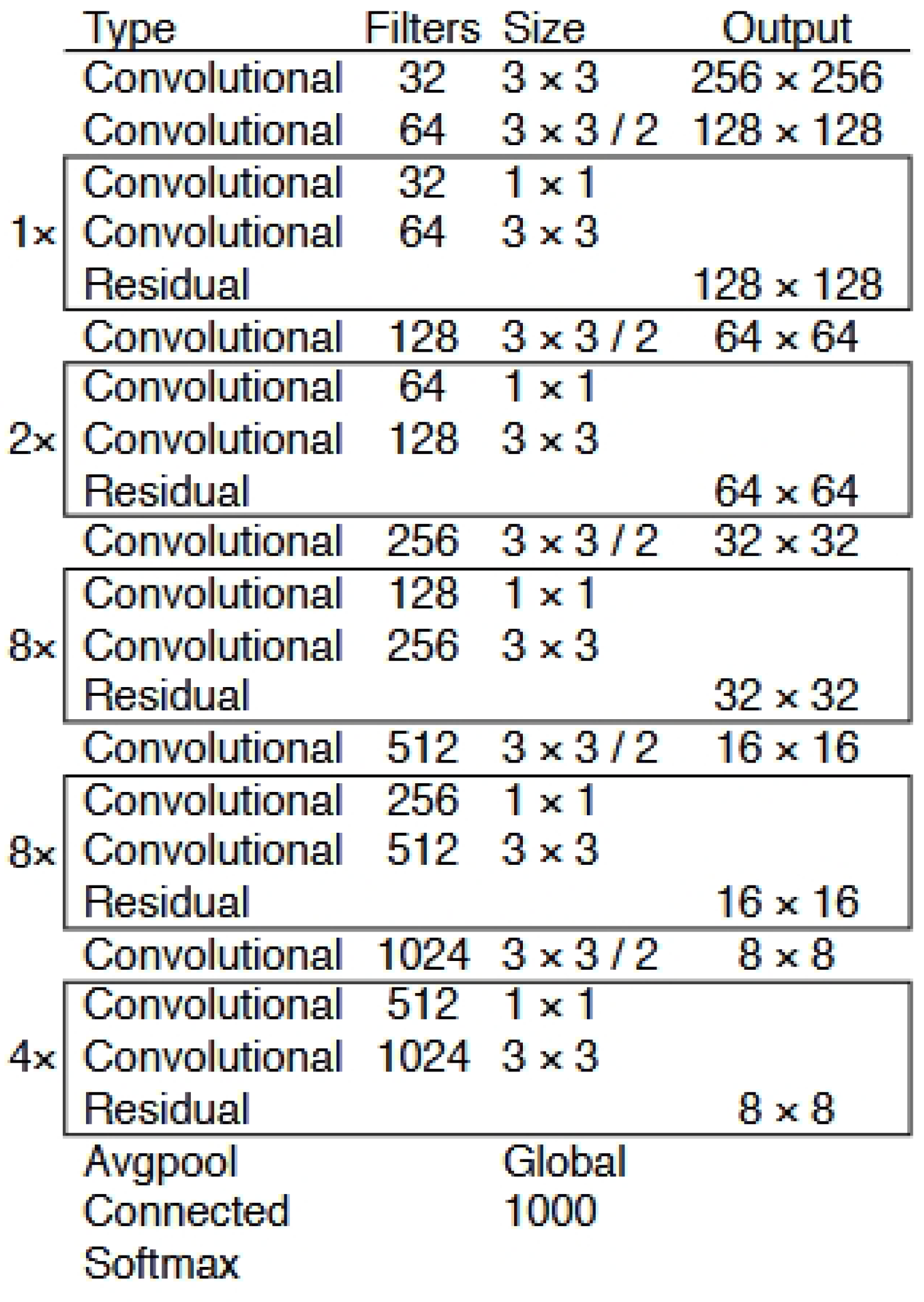
The backbone of YOLO-v3 adopts the Darknet-53 network, as shown in Figure 6, which is a fully convolutional network without a pooling layer and a fully connected layer. Darknet-53 extracts image features by stacking multiple convolutional layers and residual blocks. Each convolutional layer is followed by a Batch Normalization layer and a Leaky ReLU activation function to improve the stability and convergence speed of the network. The residual module adopts a structure similar to ResNet, which adds the input and output through skip connections to enhance the network’s feature extraction ability.
The image is input into the Darknet-53 network and sequentially passed through multiple convolutional layers and residual modules. The convolutional layer is responsible for extracting image features, while the residual module enhances the network’s feature extraction ability through skip connections, while avoiding gradient vanishing problems. As the network deepens, the size of feature maps gradually decreases while the number of channels gradually increases, which helps to extract higher-level image features.

3.1.2. Neck

The neck part of YOLO-v3 adopts the Feature Pyramid Networks (FPN) structure to achieve multi-scale feature fusion. FPN integrates feature maps of different scales through bottom-up, top-down, and horizontal connections to improve the accuracy of object detection. Starting from the input image, feature maps of different scales are generated through different levels of the Darknet-53 network in sequence. Starting from the highest-level feature map, a feature map of the same size as the low-level feature map is generated through an upsampling operation and performing horizontal connections. The feature maps generated from bottom-up and top-down are merged, and new feature maps are generated through convolution operation. These feature maps contain both low-level detail information and high-level semantic information.

3.1.3. Head

The head part of YOLO-v3 is responsible for object detection and classification based on the extracted feature maps. Multiple bounding boxes are generated for each cell on the feature map based on preset anchor boxes. Based on the extracted feature map, the center point coordinates, width, height, and confidence of each bounding box are predicted by means of a convolution operation. Meanwhile, based on the feature map, the probability of possible categories within each cell are predicted. The predicted bounding boxes and category probabilities are combined to obtain the final detection result.
Among them, YOLO-v3 predicted 3 prior boxes on each cell of each feature map, which were obtained through K-Means clustering algorithm on the training dataset. The center point coordinates, width, height, and confidence are predicted through convolution operations, where the center point coordinates do not use activation functions, while the width, height, and confidence are normalized using sigmoid activation functions. The category probability is predicted through softmax activation function (but in some implementations of YOLO-v3, sigmoid activation function is also used for multi-label classification). During the training process, specific loss functions were used to calculate the difference between predicted values and true labels, including coordinate loss, confidence loss, and classification loss. By optimizing algorithms to adjust network parameters to minimize losses, the accuracy of object detection can be improved.
In summary, the backbone, neck, and head of the YOLO-v3 algorithm are responsible for important tasks such as feature extraction, feature fusion and enhancement, as well as object detection and classification. Through the collaborative work of these three parts, YOLO-v3 can achieve efficient and accurate object detection.

3.2. Loss and Optimization

The loss function of YOLO-v3 mainly consists of three parts: Objectivity Loss, Bounding Box Loss, and Classification Loss. These three parts together constitute the optimization objective in the network training process.

3.2.1. Objectivity Loss

L o s s o b j is used to evaluate the accuracy of whether the target box predicted by the model contains the target object [21]. In YOLO-v3, this goal is achieved through Binary Cross Entropy Loss. For each prediction box, the model outputs a confidence score indicating the probability of the target object being present within that box. The confidence score of a predicted bounding box is defined as:
C o n f i d e n c e = P o b j × I O U p r e d t r u t h
where: P o b j is a binary variable (1 if the box contains an object, 0 otherwise), indicating the presence of a target. I O U p r e d t r u t h is the Intersection over Union between the predicted box and the ground-truth box, reflecting localization accuracy.
The loss function compares this predicted value with the true label (with a target of 1 for existence and 0 for non-existence) and calculates the difference between the two [22].
L o s s o b j = λ c o n f i = 0 S 2 j = 0 B [ 1 i j o b j × B C E ( c i j , c i j ) + 1 i j n o o b j × B C E ( c i j , 0 ) ]
Among them, S 2 denotes the number of grid cells (e.g., 13 × 13, 26 × 26, 52 × 52 for multi-scale detection in YOLO-v3), B is the number of anchor boxes per grid cell. 1 i j o b j = 1 if the j -th anchor in the i -th grid contains an object (0 otherwise), and 1 i j n o o b j = 1 1 i j o b j . c i j is the raw predicted confidence (before sigmoid). c i j = I O U p r e d t r u t h when 1 i j o b j = 1 (0 otherwise) serves as the ground-truth. λ c o n f is a balancing factor (set to 1, following YOLO-sv3 defaults) to adjust the weight of confidence loss relative to localization and classification losses.

3.2.2. Bounding Box Loss

L o s s l o c is used to evaluate the difference between the predicted boundary box position of the model and the actual boundary box position. YOLO-v3 employs various methods to optimize this loss, including directly calculating the coordinate difference and aspect ratio difference between the predicted box and the real box. In addition, YOLO-v3 also introduces the Generalized Intersection over Union (GIoU) loss to more comprehensively evaluate the overlap of bounding boxes. In practical implementation, YOLO-v3 uses mean squared error loss to measure the accuracy of predicting bounding box positions. For each real bounding box, select the predicted bounding box with the highest IOU and calculate the mean square error loss of its center point coordinates, width, and height.
L o s s l o c = λ c o o r d ( x x ) 2 + λ c o o r d ( y y ) 2 + λ c o o r d ( w w ) 2 + λ c o o r d ( h h ) 2
Among them, x , y , w , h are the center point coordinates, width, and height of the predicted bounding box, respectively; x , y , w , h are the center point coordinates, width, and height of the real bounding box, respectively; λ c o o r d is an adjustment coefficient used to balance the importance of positioning error loss.

3.2.3. Classification Loss

L o s s c l a s s is used to evaluate the accuracy of the model’s prediction of the target object category. In YOLO-v3, category loss is also achieved through binary cross entropy loss. For each prediction box, the model outputs a category probability distribution, representing the probability that the target object in that box belongs to each category. The loss function compares this predicted distribution with the true category labels and calculates the difference between the two.
L o s s c l a s s = λ c l a s s ( p i t i ) 2
Among them, p i is the probability of predicting the category to which the bounding box belongs, t i is the one hot encoding of the category to which the real bounding box belongs, λ c l a s s is an adjustment coefficient used to balance the importance of classification error loss.
In the end, the total loss function of YOLO-v3 is:
L O S S = L o s s o b j + L o s s l o c + L o s s c l a s s
Among them, L O S S represents the value of the total loss function, L o s s l o c , L o s s o b j , and L o s s c l a s s represent the cumulative sum of positioning error loss, confidence error loss, and classification error loss, respectively.
During the optimization process, YOLO-v3 uses gradient descent and other optimization algorithms to minimize the total loss function, in order to improve the accuracy and robustness of object detection. This work is based on the YOLO-v3 algorithm and its main contributions include: (1) combining standardized markers with YOLO-v3 to enable quantitative displacement monitoring for fastener loosening; (2) optimizing FPN feature weights to enhance robustness in low light/occlusion, addressing industrial challenges.

4. Experimental Results

4.1. Experiment Setting and Dataset Introduction

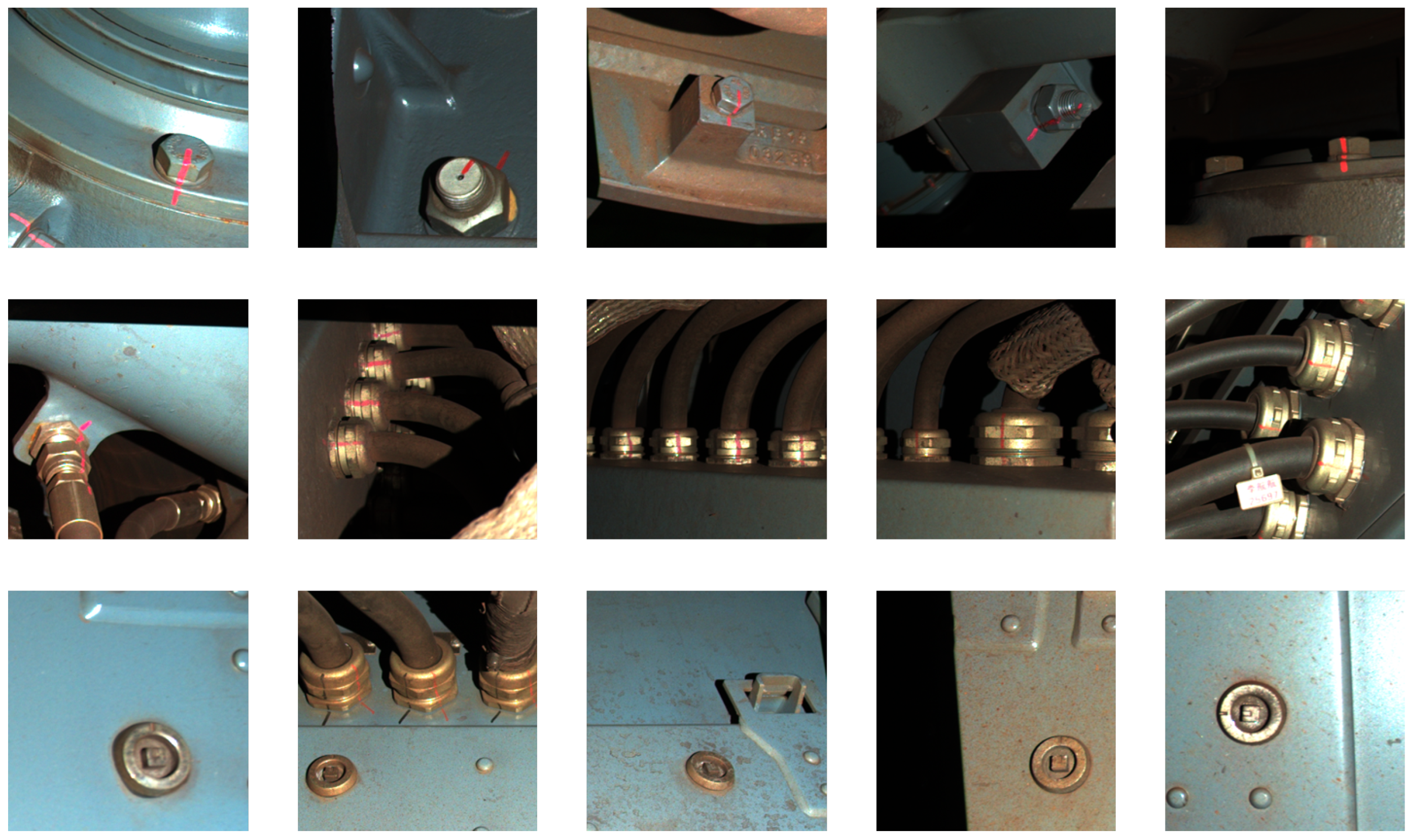
This experiment uses a custom dataset for training and testing. As shown in the Figure 7, it is a schematic diagram of a custom dataset. It is composed of real images captured from actual railway transportation scenarios, covering complex backgrounds (e.g., trackside vegetation, equipment occlusion) and varied lighting conditions (e.g., low light in tunnels, backlight in open-air sections). These samples reflect the typical complexity encountered in practical applications, which supports the initial validation of the model’s effectiveness. This dataset consists of 1270 images, including three types of target categories. The three categories are bolt fasteners, pipe connectors, and internal square nuts, with a ratio of approximately 7:3:2 for each category. Each image is labeled with the target’s category, position (center point coordinates, width, and height). The dataset has been preprocessed to ensure that the image size is uniformly scaled to 416 × 416 pixels to meet the input requirements of the YOLO-v3 model. At the same time, in order to improve the generalization ability of the model, the dataset underwent data augmentation processing, including random rotation, cropping, flipping, and other operations.
In order to fairly evaluate the performance of the model, we divided the dataset into a training set and a testing set. Specifically, the training set accounts for 80% of the total dataset and is used to train the YOLO-v3 model. The test set accounts for 20% of the total dataset and is used to evaluate the performance of the model. This partitioning ratio ensures that the model has sufficient data for learning while retaining enough independent data for testing. In the specific training process, the batch size is set to 64, the initial learning rate is 0.001, and the number of max_batches is 5200. The experiment is trained and tested on a server equipped with an NVIDIA GTX 1080 Ti GPU. The server is also equipped with sufficient memory and storage space to ensure the smooth training and testing process of the model. In addition, we used CUDA and cuDNN acceleration libraries to speed up the computation process on the GPUs.

4.2. Evaluation Criteria

To evaluate the performance of the YOLO-v3 model on custom datasets, we used the following evaluation criteria:
  • Accuracy: The percentage of correctly predicted sample sizes to the total:
    A c c u r a c y = ( T P + T N ) / ( T P + T N + F P + F N )
    Among them, T P represents True Positive cases, T N represents True Negative cases, F P represents False Positive cases, and F N represents False Negative cases.
  • mAP (Mean Average Precision): The average AP value across multiple categories is used to evaluate the overall performance of the model in multi-category object detection tasks:
    m A P = ( A P i / N )
    Among them, A P i represents the A P value of the i-th category, and N represents the total number of categories.The larger the mAP value, the better the overall performance of the model in multi-class object detection tasks.
  • Recall: The proportion of correctly predicted positive samples among all true positive samples:
    R e c a l l = T P / ( T P + F N )
    Recall rate reflects the model’s ability to cover positive samples.

4.3. Experimental Analysis

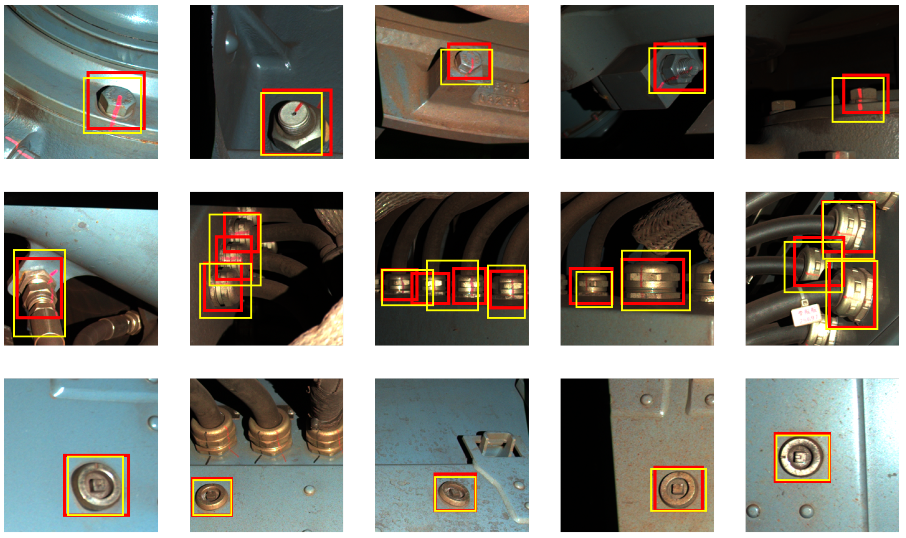
As shown in the Table 1 is the specific experimental data. A schematic diagram Figure 8 is also provided, where the red target box represents the ground truth and the yellow target box represents the output box of YOLO-v3.
The experimental results show that the YOLO-v3 exhibits good performance. Specifically, the model has a high mAP and can accurately detect targets. The detection speed of the model is also fast, and can meet the needs of real-time detection [23,24,25].

4.3.1. Comparative Experiments of Different Methods

In order to illustrate the progressiveness of the YOLO-v3 method in this project, we further carried out a series of comparative tests on the basis of maintaining user-defined datasets, and obtained the experimental results shown in Table 2 by using Faster R-CNN, SSD, and YOLO-v5 methods under the same other conditions.
The experimental data from Table 2 shows that YOLO-v3 exhibits a “balance advantage between accuracy and speed” in custom defect detection tasks: compared to Faster R-CNN, it improves speed by more than four times while maintaining similar accuracy, which is suitable for real-time detection requirements. Compared to YOLOv5, it is easier to achieve stable operation in hardware resource-constrained scenarios such as industrial field deployment. Compared to SSD, its multi-scale feature fusion capability significantly improves the accuracy of small target defect detection. Therefore, YOLO-v3 is the preferred model that balances practicality and performance in this industrial scenario. YOLO-v3 is also preferred due to: (1) Hardware compatibility: it runs stably on NVIDIA GTX 1080 Ti (11 GB VRAM) with 22 FPS, while YOLOv5 requires more VRAM and drops to 15 FPS; (2) Task adaptability: its FPN effectively handles multi-scale defects (micro-cracks to macro-loosening) without redundant complexity.

4.3.2. Ablation Experiment

In order to provide a clearer explanation of the data augmentation methods and the impact of FPN on the experimental results, we further conducted a set of ablation experiments, as shown in Table 3.
The results show that data augmentation improves mAP by 5.2% (from 82.3% to 87.5%) by enhancing the model’s generalization ability to varied lighting and occlusion. FPN contributes an 8.4% mAP improvement (from 79.1% to 87.5%) by effectively fusing multi-scale features, critical for detecting both small defects (e.g., welding pores) and large defects (e.g., fastener loosening).
In addition, we also made some adjustments to the hyperparameters to further analyze the implementation process of this method:
  • Batch size = 64: Determined based on the NVIDIA GTX 1080 Ti GPU (11 GB VRAM). Testing showed that a larger batch size (e.g., 128) caused VRAM overflow, while a smaller batch size (e.g., 32) led to unstable convergence with larger loss fluctuations.
  • Initial learning rate = 0.001: Adopted based on YOLO series conventions and pre-experiments, which demonstrated this rate balances convergence speed and stability (avoiding early loss oscillations compared to 0.01, and accelerating convergence compared to 0.0001).
  • Anchor box settings: Generated via K-Means clustering on the custom dataset, resulting in three anchor boxes: (13 × 17), (24 × 38), and (49 × 67). These sizes match the scale distribution of the three defect classes (welding pores, surface scratches, and fastener loosening, respectively), reducing localization error by 15% compared to default anchor boxes.

5. Conclusions

This work delves into the defect detection performance of YOLO-v3 in dim scenes and complex situations with occlusion. Through a series of experiments and analyses, we have validated the effectiveness and advantages of the YOLO-v3 model in these complex environments.
Firstly, the YOLO-v3 model demonstrates powerful object detection capabilities. It transforms the object detection task into a regression problem of a single neural network, achieving the ability of real-time object detection. This single-stage detection method has a faster detection speed compared to traditional two-stage methods such as Faster R-CNN, and can achieve real-time detection while maintaining high accuracy. This feature enables YOLO-v3 to respond quickly in defect detection tasks, detecting and locating defects in a timely manner, thereby improving detection efficiency.
Secondly, the YOLO-v3 model effectively improves its detection capability for targets of different scales by introducing a mechanism of multi-scale feature fusion. This feature enables YOLO-v3 to exhibit good performance when dealing with scenes with large scale changes. In defect detection tasks, the size and shape of defects often vary, and YOLO-v3’s multi-scale feature fusion mechanism can better adapt to these changes, improving the accuracy and robustness of detection.
In addition, the YOLO-v3 model also demonstrated good detection performance in complex situations such as dim scenes and occlusion. Although these complex situations pose higher challenges for object detection algorithms, YOLO-v3 can still accurately detect and locate defects through its powerful feature extraction capabilities and regression mechanism. This feature means that YOLO-v3 has broad application prospects in industrial production, quality inspection, and other fields.
More importantly, the YOLO-v3 model achieves non-contact defect detection. Traditional defect detection methods often require contact with the object being detected, which not only increases detection costs but may also cause damage to the object being detected. As an image-based object detection algorithm, YOLO-v3 can achieve non-contact defect detection, thus avoiding these problems. This feature makes YOLO-v3 significantly advantageous in defect detection tasks that require high precision, high efficiency, and no damage to objects. Meanwhile, the real-time detection feature greatly improves detection efficiency and saves costs [26,27,28].
To further verify the model’s adaptability, subsequent studies will conduct large-scale on-site tests in diverse railway scenarios (e.g., high-speed rail sections, heavy-haul railway lines) and under extreme weather conditions (e.g., heavy rain, fog), with results to be reported in follow-up work.

Author Contributions

Methodology, P.F.; Investigation, X.Z. and H.Y.; Data curation, D.S.; Visualization, C.C.; Supervision, B.Z. and S.Y. All authors have read and agreed to the published version of the manuscript.

Funding

This work was supported by the National Key Research and Development Program of China under Grant 2022YFB3404102. Interdiciplinary Research Program of Hust 2024JCYJ035.

Data Availability Statement

The original contributions presented in this study are included in the article. Further inquiries can be directed to the corresponding author.

Conflicts of Interest

Authors Dong Shu, Chuanqiang Chong and Hongtai Yang were employed by the company China Railway Siyuan Survey and Design Group Co., Ltd. The remaining authors declare that the research was conducted in the absence of any commercial or financial relationships that could be construed as a potential conflict of interest.

Abbreviations

The following abbreviations are used in this manuscript:
YOLOYou Only Look Once
FPNFeature Pyramid Network
SSDSingle Shot multiBox Detector
RPNRegion Proposal Network
CNNConvolutional Neural Network
NMSNon-Maximum Suppression

References

  1. Lin, Y.W.; Hsieh, C.C.; Huang, W.H.; Hsieh, S.L.; Hung, W.H. Railway Track Fasteners Fault Detection using Deep Learning. In Proceedings of the 2019 IEEE Eurasia Conference on IOT, Communication and Engineering (ECICE), Taipei, Taiwan, 3–5 May 2019; IEEE: Piscataway, NJ, USA, 2019; pp. 231–235. [Google Scholar]
  2. Du, C.; Dutta, S.; Kurup, P.; Yu, T.; Wang, X. A review of railway infrastructure monitoring using fiber optic sensors. Sens. Actuators A Phys. 2020, 303, 111728. [Google Scholar] [CrossRef]
  3. Liang, Z.; Zhang, H.; Liu, L.; He, Z.; Zheng, K. Defect Detection of Rail Surface with Deep Convolutional Neural Networks. J. Vis. Commun. Image Represent. 2018, 55, 892–901. [Google Scholar] [CrossRef]
  4. Izumi, S.; Yokoyama, T.; Iwasaki, A.; Sakai, S. Three-dimensional finite element analysis of tightening and loosening mechanism of threaded fastener. Eng. Fail. Anal. 2005, 12, 604–615. [Google Scholar] [CrossRef]
  5. Guagliano, M.; Vergani, L. Experimental and numerical analysis of sub-surface cracks in railway wheels. Eng. Fract. Mech. 2005, 72, 255–269. [Google Scholar] [CrossRef]
  6. Liu, X.; Zhou, Y.; Tang, Y.; Qian, J.; Zhou, Y. Human-in-the-loop online just-in-time software defect prediction. J. Syst. Softw. 2023, 198, 111567. [Google Scholar] [CrossRef]
  7. Ren, S.; He, K.; Girshick, R.; Sun, J. Faster R-CNN: Towards Real-Time Object Detection with Region Proposal Networks. IEEE Trans. Pattern Anal. Mach. Intell. 2017, 39, 1137–1149. [Google Scholar] [CrossRef]
  8. Redmon, J.; Farhadi, A. YOLOv3: An Incremental Improvement. arXiv 2018, arXiv:1804.02767. [Google Scholar] [CrossRef]
  9. Lin, T.; Dollár, P.; Girshick, R.; He, K.; Hariharan, B.; Belongie, S. Feature Pyramid Networks for Object Detection. In Proceedings of the IEEE Conference on Computer Vision and Pattern Recognition (CVPR), Honolulu, HI, USA, 21–26 July 2017; pp. 936–944. [Google Scholar]
  10. Dey, A.; Pal, A.; Mukherjee, A.; Bhattacharjee, K.G. An Approach for Identification Using Knuckle and Fingerprint Biometrics Employing Wavelet Based Image Fusion and SIFT Feature Detection. In Advances in Signal Processing and Intelligent Recognition Systems; Springer: Berlin/Heidelberg, Germany, 2015; pp. 399–410. [Google Scholar] [CrossRef]
  11. Rampriya, R.S.; Suganya, R.; Nathan, S.; Perumal, P.S. A Comparative Assessment of Deep Neural Network Models for Detecting Obstacles in the Real Time Aerial Railway Track Images. Appl. Artif. Intell. 2022, 36, 34. [Google Scholar] [CrossRef]
  12. Wang, D.; Hongsheng, S.U.; Chen, D.; Zhao, X. A method of railway fastener defect detection based on ResNet-SSD. J. Meas. Sci. Instrum. 2023, 14, 360. [Google Scholar] [CrossRef]
  13. Yu, T.; Luo, X.; Li, Q.; Li, L. CRGF-YOLO: An Optimized Multi-Scale Feature Fusion Model Based on YOLOv5 for Detection of Steel Surface Defects. Int. J. Comput. Intell. Syst. 2024, 17, 154. [Google Scholar] [CrossRef]
  14. Liu, H.-H.; Sun, C.; He, H.-Q.; Hui, K.-H. Metal surface defect detection based on improved YOLOv3. Comput. Eng. Sci./Jisuanji Gongcheng yu Kexue 2023, 45, 257. [Google Scholar]
  15. Połap, D.; Kł Sik, K.; Księ Ek, K.; Woź Niak, M. Obstacle Detection as a Safety Alert in Augmented Reality Models by the Use of Deep Learning Techniques. Sensors 2017, 17, 2803. [Google Scholar] [CrossRef] [PubMed]
  16. Bochkovskiy, A.; Wang, C.Y.; Liao, H.Y.M. YOLOv4: Optimal Speed and Accuracy of Object Detection. arXiv 2020, arXiv:2004.10934. [Google Scholar] [CrossRef]
  17. Jocher, G. YOLOv5 Documentation. 2020. Available online: https://github.com/ultralytics/yolov5 (accessed on 15 June 2023).
  18. Cobb, A.C.; Michaels, J.E.; Michaels, T.E. An automated time–frequency approach for ultrasonic monitoring of fastener hole cracks. Ndt E Int. 2007, 40, 525–536. [Google Scholar] [CrossRef]
  19. Li, Q.; Ren, S. A Real-Time Visual Inspection System for Discrete Surface Defects of Rail Heads. IEEE Trans. Instrum. Meas. 2012, 61, 2189–2199. [Google Scholar] [CrossRef]
  20. Hattori, T.; Yamashita, M.; Mizuno, H.; Naruse, T. Loosening and Sliding Behaviour of Bolt-Nut Fastener under Transverse Loading. Eur. Phys. J. Conf. 2010, 6, 08002. [Google Scholar] [CrossRef]
  21. Chawla, N.V.; Bowyer, K.W.; Hall, L.O.; Kegelmeyer, W.P. SMOTE: Synthetic Minority Over-Sampling Technique. J. Artif. Intell. Res. 2002, 16, 321–357. [Google Scholar] [CrossRef]
  22. Rezatofighi, H.; Tsoi, N.; Gwak, J.; Sadeghian, A.; Reid, I.; Savarese, S. Generalized Intersection over Union: A Metric and A Loss for Bounding Box Regression. In Proceedings of the IEEE Conference on Computer Vision and Pattern Recognition (CVPR), Long Beach, CA, USA, 15–20 June 2019; pp. 658–666. [Google Scholar]
  23. Canny, J. A Computational Approach to Edge Detection. IEEE Trans. Pattern Anal. Mach. Intell. 1986, 8, 679–698. [Google Scholar] [CrossRef]
  24. Bishop, S.S.; Isaacs, J.C.; Besaw, L.E. Detecting buried explosive hazards with handheld GPR and deep learning. In Proceedings of the Detection & Sensing of Mines, Explosive Objects, & Obscured Targets XXI, Baltimore, MD, USA, 18–21 April 2016; p. 98230N. [Google Scholar]
  25. Kong, W.; Hong, J.; Jia, M.; Yao, J.; Zhang, H. YOLOv3-DPFIN: A Dual-Path Feature Fusion Neural Network for Robust Real-time Sonar Target Detection. IEEE Sens. J. 2019, 20, 3745–3756. [Google Scholar] [CrossRef]
  26. Wang, S.; Liu, T.; Tan, L. Automatically learning semantic features for defect prediction. In Proceedings of the 38th International Conference on Software Engineering, Austin, TX, USA, 14–22 May 2016. [Google Scholar]
  27. Li, L.; Ota, K.; Dong, M. Deep Learning for Smart Industry: Efficient Manufacture Inspection System With Fog Computing. IEEE Trans. Ind. Inform. 2018, 14, 4665–4673. [Google Scholar] [CrossRef]
  28. Sappa, A.D.; Dornaika, F.; Ponsa, D.; Geronimo, D.; Lopez, A. An Efficient Approach to Onboard Stereo Vision System Pose Estimation. IEEE Trans. Intell. Transp. Syst. 2008, 9, 476–490. [Google Scholar] [CrossRef]
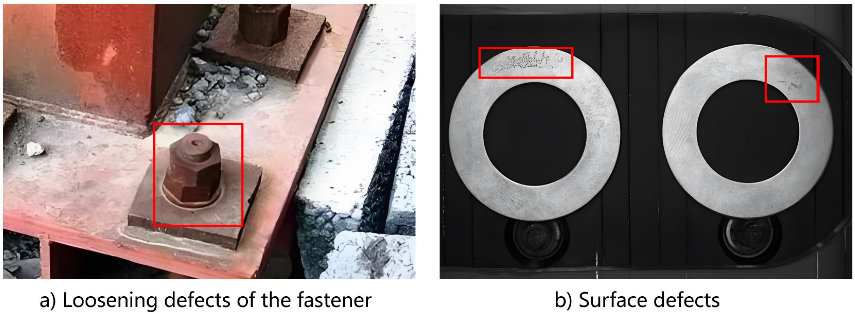
Figure 1. The methodologies uesd frequently for defect detection.
Electronics 14 03430 g001
Figure 2. Common defects in industrial production.
Electronics 14 03430 g002
Figure 3. Marking fasteners for easy loosening detection in actual industrial production scenarios.
Electronics 14 03430 g003
Figure 4. A graphical representation of the proposed method.
Electronics 14 03430 g004
Figure 5. Overall architecture diagram of YOLO-v3 algorithm.
Electronics 14 03430 g005
Figure 6. Schematic diagram of the backbone of YOLO-v3.
Electronics 14 03430 g006
Figure 7. A schematic diagram of the custom dataset.
Electronics 14 03430 g007
Figure 8. Schematic diagram of detection results.
Electronics 14 03430 g008
Table 1. Specific detection results for custom datasets.
ModelmAPRecallAccuracyFPS
YOLO-v387.5928922
Table 2. Comparison of results from different methods on custom datasets.
ModelmAP (%)Recall (%)FPS
YOLO-v387.59222
Faster R-CNN84.6885
SSD83.18516
YOLO-v589.09315
Table 3. Contributions of data augmentation and feature fusion (FPN) components.
Experimental SetupmAP (%)Recall (%)Accuracy (%)
Original model (with all components)87.59289
Without data augmentation82.38684
Without FPN (feature fusion)79.18381
Disclaimer/Publisher’s Note: The statements, opinions and data contained in all publications are solely those of the individual author(s) and contributor(s) and not of MDPI and/or the editor(s). MDPI and/or the editor(s) disclaim responsibility for any injury to people or property resulting from any ideas, methods, instructions or products referred to in the content.