1. Introduction
We are currently witnessing the robust development of the Internet of Things (IoT) [
1,
2,
3,
4,
5,
6], big data, and artificial intelligence technologies. As a result, the global manufacturing industry is accelerating its shift towards an intelligent era. In this transformation, we find that conducting real-time monitoring of the entire industrial production process and making data-driven decisions are essential. These actions are crucial for boosting industrial efficiency. Furthermore, they play a key role in improving product quality. Metallic materials, being the foundation of modern industry, have a direct impact on the reliability and safety of downstream products. Many industries, such as wire, construction, and equipment manufacturing, are closely associated with metallic materials [
7].
Steel, a type of metallic material, often develops various defects during production. If not detected promptly and used in industrial applications, these defective products can affect the appearance and corrosion resistance of products. In severe cases, they may even pose serious safety risks [
8]. Therefore, an effective steel defect detection algorithm is of great significance.
Traditional detection methods, like manual visual inspection, have several drawbacks. These include low efficiency, low accuracy, and susceptibility to human factors, making them unsuitable for modern industrial production requirements. Machine-learning-based detection methods also face issues. For example, they are time-consuming in feature extraction, have poor results, limited generalization ability, low computational efficiency, and often fail to achieve the desired outcomes [
9].
In recent years, deep learning technology has advanced rapidly [
10]. Convolutional neural networks (CNNs) have found extensive applications in various practical fields [
11], especially excelling in image recognition and detection. Traditional detection methods are inefficient and inaccurate, while deep learning technology offers new solutions and breakthroughs for steel surface defect detection [
12].
Leng Yuefeng et al. [
13] proposed an improved Faster R-CNN algorithm. They introduced a feature fusion module and a lightweight channel attention module between FPN and RPN. This enhanced the model’s ability to capture fine features and improved detection accuracy. Kou et al. [
14] designed an end-to-end defect detection model based on YOLOv3. They incorporated a specially designed dense convolution block, which improved the model’s detection performance. Zhao et al. [
15] added the Res2Net block to the backbone network of YOLOv5 and designed a dual feature pyramid network (DFPN) to enhance the neck structure. This deepened the network and enabled it to reuse low-level features, thus improving the model’s detection performance. Wang Mengyu et al. [
16] put forward the ADP-YOLOv8. They enhanced the model’s sensitivity to multi-scale defects and improved detection accuracy through an adaptive weight downsampling module, an improved C2f module, and the introduction of a programmable gradient information module. Cui Kebin et al. [
17] proposed the MCB-FAH-YOLOv8 algorithm. They introduced an improved CBAM and a replaceable four-head ASFF prediction head, optimizing feature extraction and fusion strategies and enhancing detection accuracy and robustness. Song X et al. [
18] added C2f_DCNv2 and a Biformer attention mechanism to YOLOv8, improving the model’s accuracy in steel surface defect detection.
However, most deep-learning-based model training and testing require devices with sufficient memory and computing resources. In actual production, device computing power may be insufficient, resulting in poor model deployability on mobile detection devices. Although previous research has boosted the detection accuracy in steel defect detection models to some extent, issues such as voluminous parameters and heavy computational burden still remain. In the actual production process, we need algorithms that balance detection accuracy and deployability and have strong real-time performance [
19,
20,
21,
22,
23].
In summary, we propose a lightweight algorithm for steel surface defect detection based on YOLOv8n herein. Our contributions include the following:
We added a new set of upsampling and feature fusion layers to the neck of YOLOv8. This enhances the model’s feature extraction and fusion abilities. It allows the model to combine more feature information from different levels, improving the steel defect detection model’s ability to capture defect features.
In the neck, we fused the bottleneck module of the C2f module and the RepVit Block of the RVB module to form a new module, C2f_RVB. This effectively reduces model complexity. At the same time, it can capture the key information in the input image more accurately.
We introduced an improved GAM-B attention mechanism before the SPPF module. This enables the network model to focus on the image’s key information from both channel and spatial dimensions. As a result, the network’s ability to recognize steel surface defects is improved.
In the detection head, we optimized the pre-existing detection head using the concept of weight sharing and group convolution. This significantly reduces the complexity of the steel defect detection model and improves the detection accuracy.
2. The Network Architecture of YOLOv8
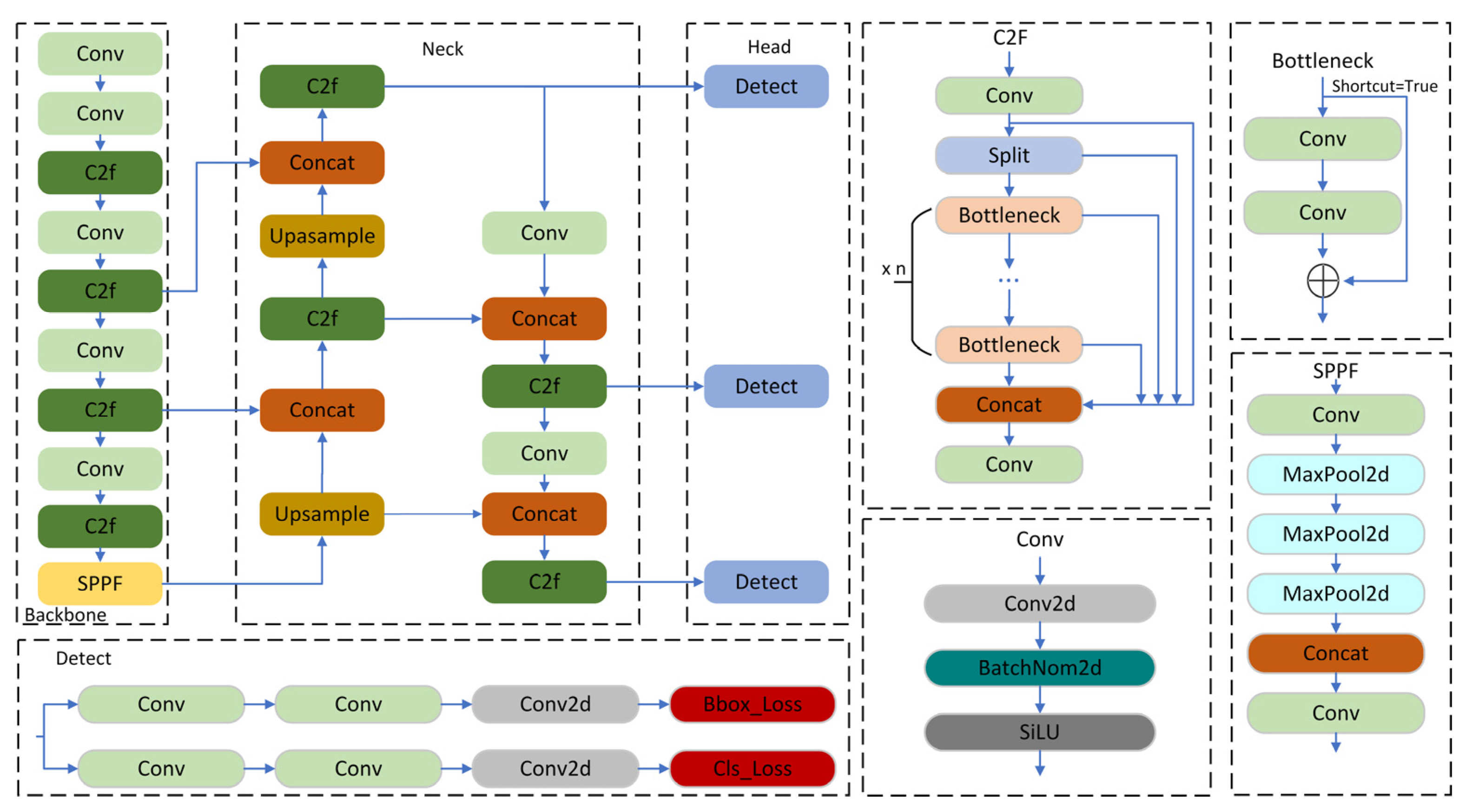
The network architecture of YOLOv8 consists of three parts: backbone, neck, and head. As an improved version of YOLOv5, YOLOv8 adopts the gradient separation concept in both the backbone and neck structures and also utilizes the PAN-FPN structure [
24,
25]. Inspired by the ELAN module in YOLOv7 [
26], YOLOv8 replaces the C3 module in YOLOv5 with a more lightweight C2f module. Moreover, YOLOv8 modifies the decoupled head structure of the head. It separates the classification and localization tasks and adopts an Anchor-Free methodology. These improvements further enhance the model’s flexibility and accuracy. As a result, YOLOv8 shows better performance in object detection tasks and has greater adaptability to targets of different sizes and shapes.
Figure 1 illustrates the overall architecture of YOLOv8.
3. The Object Detection Network of PPY-YOLO
The official YOLOv8 offers five versions: YOLOv8n, YOLOv8s, YOLOv8m, YOLOv8l, and YOLOv8x. Given the need for a lightweight and highly real-time steel defect detection model in actual steel production, this paper uses YOLOv8n as the baseline for improvement.
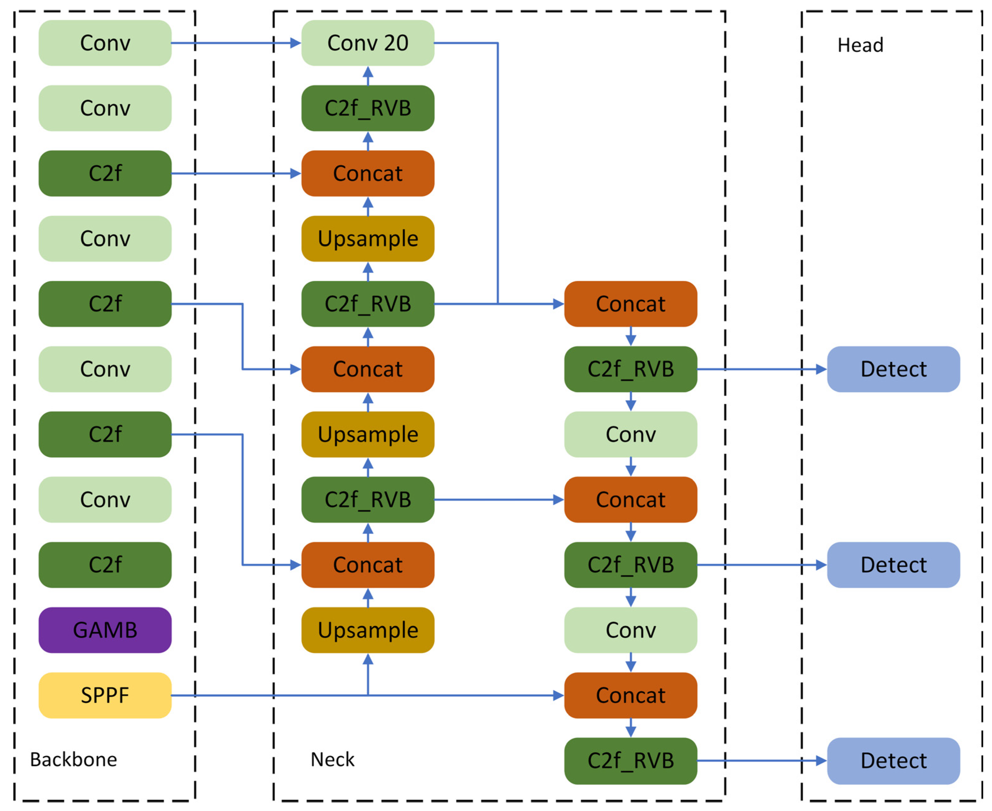
The architecture of the improved network PPY-YOLO is presented in
Figure 2. The whole network consists of three parts: backbone, neck, and head.
3.1. Improvement of the Neck
In the practical applications of steel defect detection, the surface of the steel strip often has complex background textures, illumination changes, and potential mechanical scratches and other interfering factors. These complex backgrounds significantly increase the difficulty of detecting small-target defects in steel.
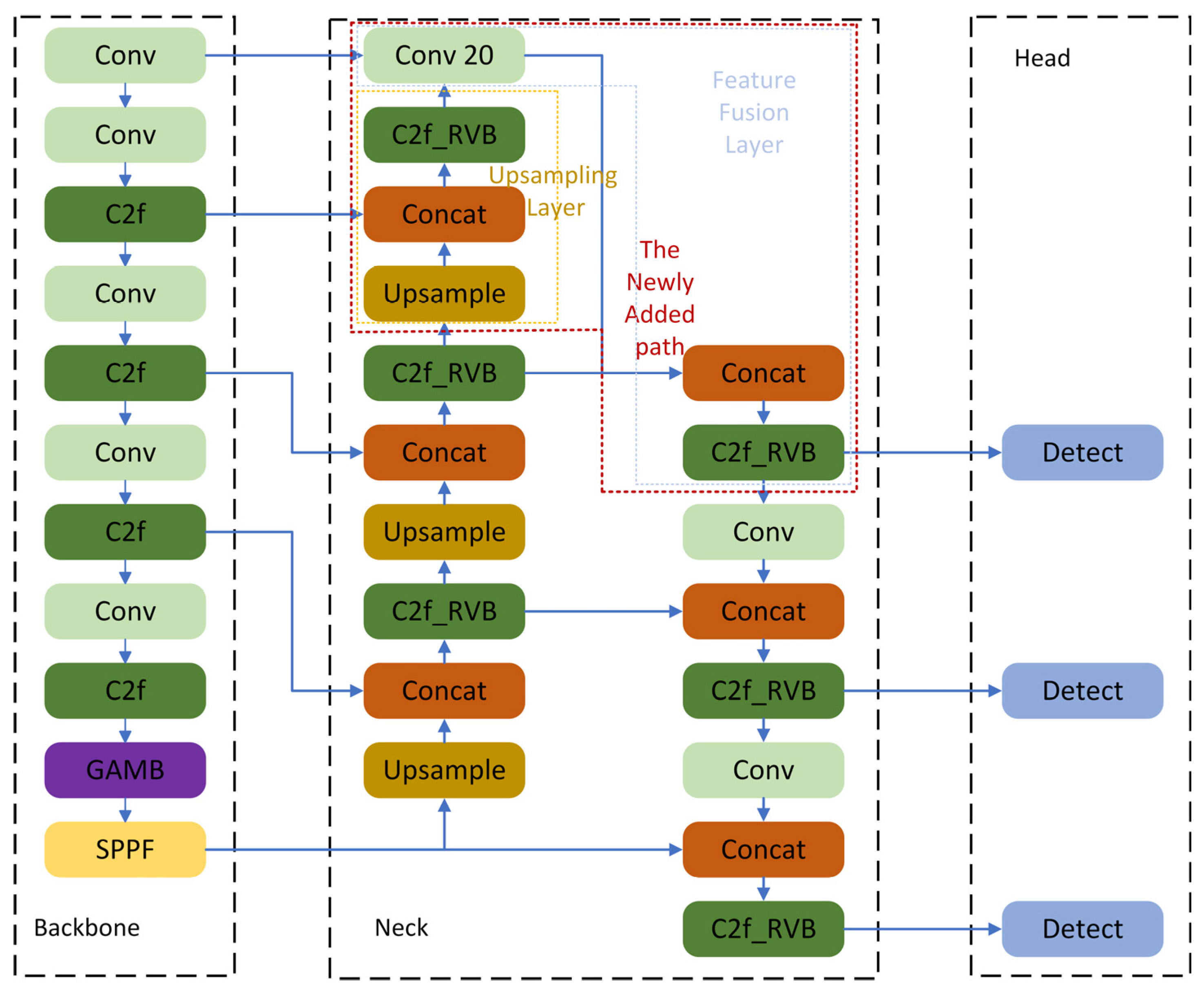
Therefore, this paper adds a group of upsampling fusion layers and feature extraction fusion layers to the neck structure of YOLOv8n. This addition aims to identify and locate small-target defects in steel more comprehensively and accurately.
As the box in
Figure 3 shows, this paper introduces a new path. In deep learning, different network layers can capture image information at different scales. Shallow features, being closer to the original input image, are more sensitive to detailed image information like edges and textures. For small-target defects on the steel surface, this detailed information is often crucial for distinguishing defects from the background.
To fully leverage the advantages of shallow features, this paper first inserts a group of upsampling fusion layers in the newly added path. These upsampling fusion layers can increase the resolution of the feature map through upsampling. They can also align and fuse it with shallow features in space via feature fusion operations. Feature fusion, an important technique in deep learning, combines features from different layers, allowing for a comprehensive utilization of each layer’s advantages to form a more complete and representative feature representation. This process not only preserves the rich detailed information in shallow features but also provides more spatial context information for subsequent defect detection by further enhancing the feature map’s resolution. As a result, the model extracts more complete features, improving the detection performance.
Moreover, this paper further adds a feature extraction fusion layer. This layer integrates the detailed features from shallow layers and the semantic features from deep layers. Eventually, it effectively fuses the detailed information from earlier layers and the abstract high-level features from deeper layers, strongly supporting the accurate detection of small-target defects in steel.
3.2. The Improved GAM-B Attention Mechanism
In the field of steel material surface defect detection, the attention mechanism is a key technology for enhancing the model’s detection performance. As a comprehensive attention mechanism, GAM (Global Attention Module) [
27] redesigned two sub-modules: the channel attention mechanism and the spatial attention mechanism based on the CBAM attention mechanism [
28]. By integrating global spatial information and channel information simultaneously, GAM can significantly boost the model’s ability to focus on key regions in the image.
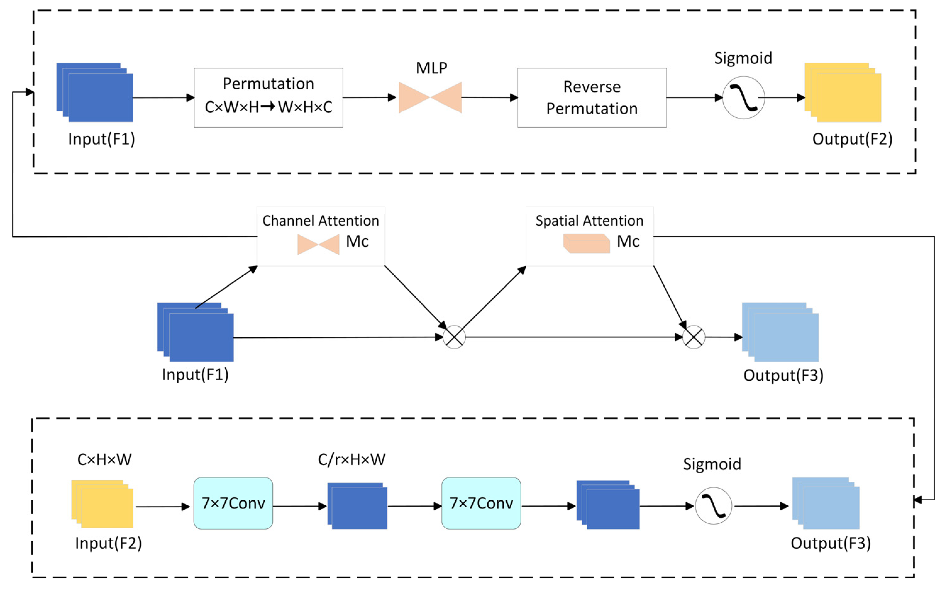
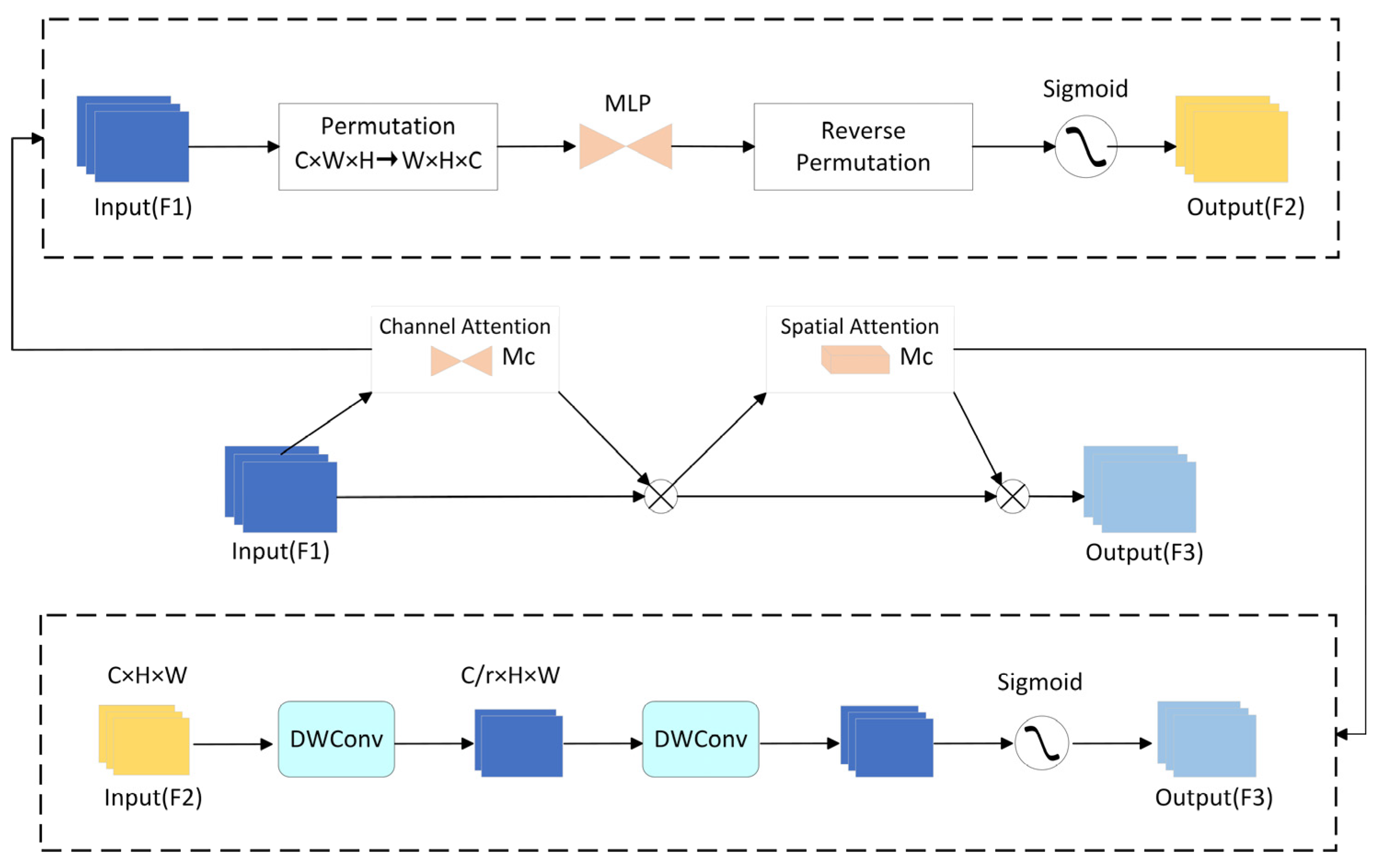
Figure 4 shows the structure of the GAM attention mechanism.
First, in the channel attention [
29] sub-module, perform a permutation operation on the input feature map
. This operation generates new feature information with a size of W × H × C. Next, use a two-layer multi-layer perceptron (MLP) [
30] to strengthen the cross-dimensional channel-spatial dependencies. Finally, obtain the output feature map
through the inverse permutation operation and the Sigmoid activation function.
Regarding the spatial attention sub-module, use two 7 × 7 standard convolutional layers to fuse the spatial feature information of the output feature map . This facilitates a more extensive acquisition of spatial features. Eventually, derive the final output feature map through the Sigmoid activation function.
Assume the input feature is
, the feature obtained after channel attention is
, and the final output feature is
. Denote the channel attention sub-module as
and the spatial attention sub-module as
. Then, we have
In fine visual tasks like the surface defect detection of steel materials, capturing and processing spatial details are of particular importance. Thus, this paper optimizes the spatial attention sub-module in GAM. Drawing inspiration from the large-kernel attention mechanism (LSKA), we enhance the spatial feature extraction capability by using a decomposed large kernel [
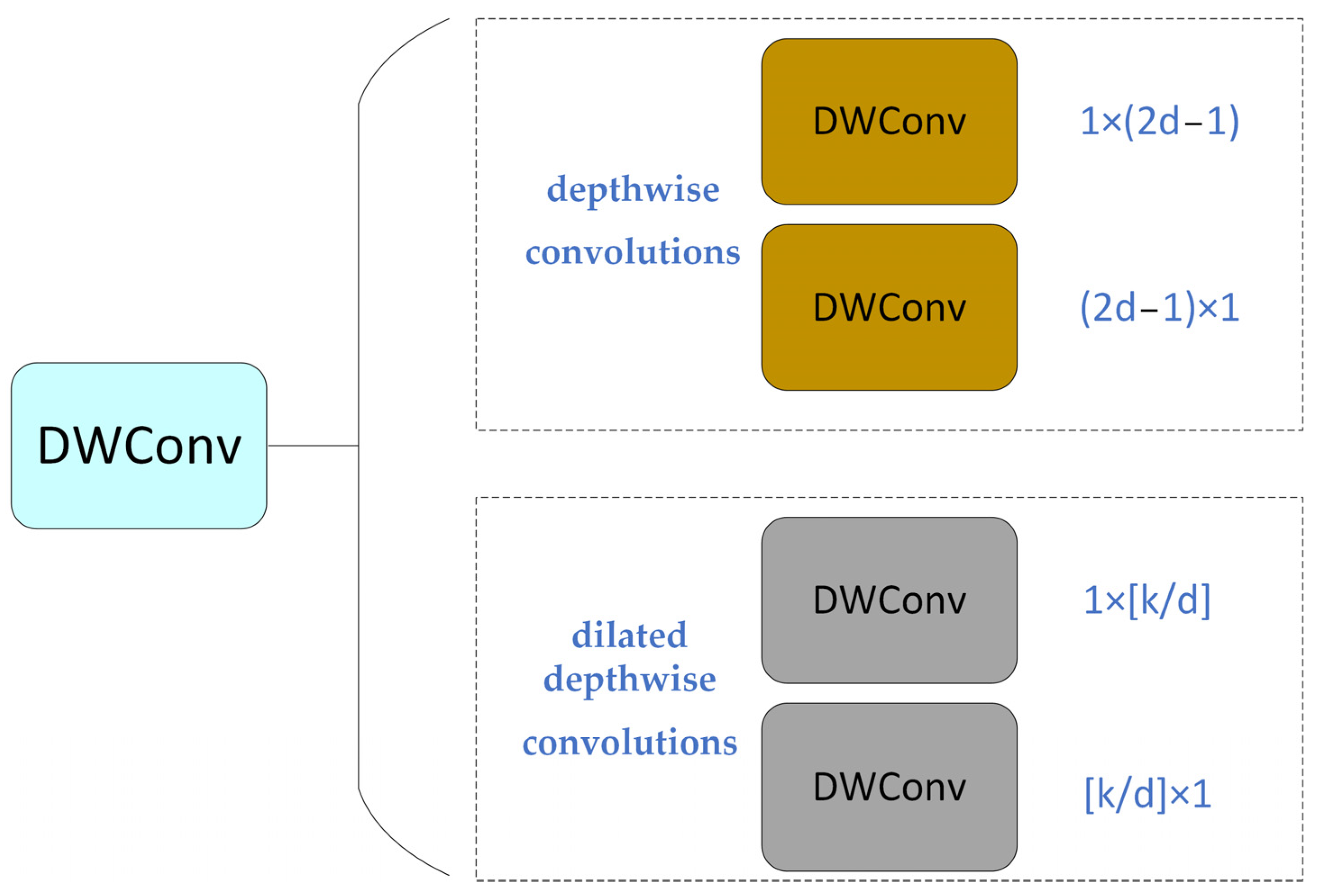
31]. Specifically, this paper replaces the two 7 × 7 standard convolution layers in the original GAM attention mechanism with two DWConv groups. Each group consists of two depthwise convolutions, one BatchNorm layer, one ReLU layer, and two dilated depthwise convolutions. The structure is presented in
Figure 5.
This modification keeps GAM’s channel attention advantages. It also boosts the model’s spatial detail sensitivity by adding depthwise convolution.
Depthwise convolution does separate convolution for each input channel, keeping channel independence. With the same receptive field, the model’s spatial attention sub-module can fully focus on extracting spatial features in each channel. So, more detailed features for steel surface defect detection are retained.
Also, the substitution of conventional convolution with depthwise convolution substantially lowers the computational complexity and parameter count [
32].
The output of the DWConv Group can be obtained as follows, assuming the input feature map is X:
where
,
,
, and
are the learnable parameters of the corresponding convolutional layers, respectively, and
denotes the depthwise convolution operation.
This improves the model’s training efficiency and reduces resource consumption during deployment. This is of significant importance for industrial defect detection scenarios that demand high real-time performance and deployability.
Figure 6 shows the structural diagram of the improved GAM-B attention mechanism.
3.3. C2f_RVB Block
The design inspiration of RepViT comes from deeply mining and innovatively integrating the intrinsic potential of lightweight visual models. It cleverly balances the efficiency of pure lightweight CNNs on mobile devices and the excellent performance of ViT networks in visual tasks. Also, it avoids ViT’s drawback of being unsuitable for resource-constrained scenarios due to its large number of parameters and high latency. With a carefully designed architecture, RepViT combines the capacity for localized feature extraction inherent in CNNs and the global contextual understanding offered by ViTs.
The RepViT Block [
33] is derived by optimizing the MobileNetV3 Block [
34]. The original MobileNetV3 Block has a 1 × 1 expansion convolution (EConv), a depthwise convolution, and a 1 × 1 projection layer. The 1 × 1 expansion and projection layers enable channel interaction, while the depthwise convolution fuses spatial information. RepViT improves channel and feature mixing. It does this by adjusting the depthwise convolution position and adding an SE layer [
35], thus enhancing performance. Furthermore, it uses the structural reparameterization technique. During training, it constructs a multi-branch topology for better performance. During inference, it merges the depthwise convolution’s multi-branch structure into one branch. This removes extra computational and memory costs from multiple branches and boosts efficiency.
In YOLOv8, the C2f module improves the model’s fine feature and context information extraction ability. However, stacking too many bottlenecks makes the C2f module’s computational complexity unable to meet the high demands for model lightweight and high computational efficiency in steel surface defect detection.
Therefore, in this paper, we replace the two standard convolution blocks with residual connections in the YOLOv8n C2f module with the RepViT Block module. Then, we fuse them into a new lightweight module, C2f_RVB. We use the C2f_RVB module to replace the C2f module in the YOLOv8n’s neck. The C2f_RVB module can maintain the ability to capture detailed information. It also optimizes multi-scale feature extraction and suppresses background noise. This allows the network to achieve higher detection accuracy in complex scenarios. Meanwhile, with a more efficient feature processing mechanism, it reduces the computational burden. It balances performance and resource utilization effectively, making the network better suited for deployment on resource-restricted platforms.
Figure 7 shows the structure diagram of the C2f_RVB module.
3.4. The Reconstruction of the Detection Head
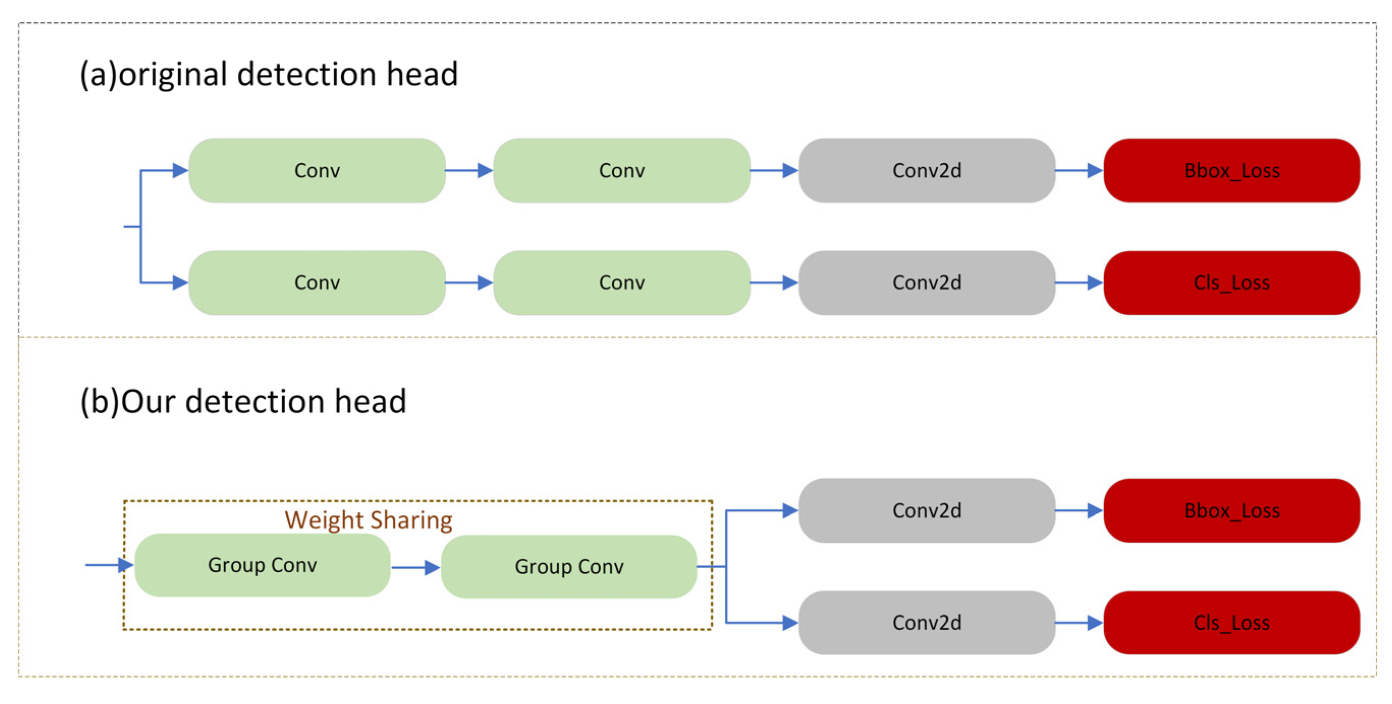
YOLOv8n differs from its previous versions in using decoupled detection heads. The structure of YOLOv8n’s detection head is shown in
Figure 8a.
The feature map passes through two branches, fulfilling classification and localization functions, respectively. Each branch consists of two 3 × 3 convolutions and one 1 × 1 convolution.
Compared with previous YOLO versions, while the decoupled detection head reduces the confusion and mutual interference of classification and localization features, thus improving accuracy, the three detection heads have twelve 3 × 3 convolutions and six 1 × 1 convolutions. This significantly increases the parameter count; this also affects the computational overhead of the detection head.
For this reason, this paper redesigns the YOLOv8n detection head. We merge the standard convolutions in the first half of the original detection head branches using the weight-sharing idea. We also use group convolutions to replace standard convolutions, further lightening the detection head. This retains the original decoupled detection head’s advantage in separating classification and localization and improves the model’s computational efficiency.
We replace all three detection heads in the YOLOv8n network with the redesigned ones, significantly reducing the network’s number of parameters and computational load.
Figure 8b shows the structure of the redesigned detection head.
4. Experiment and Analysis
4.1. Experimental Configuration
The experimental environment is Linux, the CPU is an Intel Xeon 8255C, the GPU is an RTX 2080 Ti, we used Python version is 3.8, and the deep learning framework is PyTorch 1.13.1 with CUDA 11.3. We used an initial learning rate of 0.01, a momentum of 0.937, a weight decay of 0.0005, and 400 training epochs, while the batch size was set to 16. We employed the SGD optimizer. The resolution of the input image is preprocessed to 640 × 640.
4.2. Dataset and Evaluation Metric
For the experiment, we use the NEU-DET steel surface defect dataset from Northeastern University [
36]. This dataset has six typical surface defects of hot-rolled steel strips: rolled-in scale (RS), patches (Pa), crazing (Cr), pitted surface (PS), inclusion (In), and scratches (Sc).
The dataset contains 1800 grayscale images.
Figure 9 shows the sample instance graphs of each defect type. In this paper, we partition the dataset into a training set, a validation set, and a test set in the ratio of 8:1:1. Finally, the training set has 1440 samples, the validation set has 180 samples, and the test set has 180 samples.
We evaluate the model performance using six metrics: precision, recall, mean average precision (mAP), inference speed (FPS), parameter quantity (Params), and computational complexity (GFLOPs). The calculation formulas are as follows.
Precision is the proportion of correct detection results among samples detected as positive. The formula is as follows:
Recall represents the fraction of true positive predictions out of all actual positive instances. The formula is as follows:
Among them, TP, FP, and FN, respectively, represent True Positive, False Positive, and False Negative.
The mean average precision (mAP) measures the detection accuracy and comprehensiveness of different classes. The formulas are:
where AP is the accuracy of a single class, mAP is the result of integrating the area under the PR curve, representing the mean accuracy of all classes, and
n is the number of classes. In this study, when the IoU threshold is 0.5, mAP@0.5 stands for the mAP value. Higher mAP@0.5 values indicate better detection results for different types of detection targets. mAP@0.5:0.95 averages the mAP across multiple IoU thresholds (from 0.5 to 0.95, with a 0.05 step). This accounts for the model’s performance at various IoU thresholds, providing a more comprehensive assessment.
FPS represents the model’s inference speed. Let
be the image preprocessing time,
be the image inference time, and
be the image postprocessing time. The formula is as follows:
The number of parameters (Params) refers to the parameters that need to be learned during the model training process of the network, representing the spatial complexity of the model. The larger the number of parameters, the more memory the model occupies.
Computational complexity (GFLOPs) refers to the number of floating-point operations of the model, which is used to measure the computational efficiency of the model.
4.3. Results of the Experiment and Analysis
4.3.1. Ablation Experiment
To verify the validity and effectiveness of our algorithm and each improvement, we performed ablation experiments on the improved modules using the NEU-DET dataset. Then, we assessed the improvement effect of these modules on the algorithm’s detection performance.
The experimental results are presented in
Table 1. Compared with the baseline YOLOv8n, when we improve the neck to New-Neck, the network slightly increases its FLOPs. However, the number of parameters remains nearly the same, and the mAP@0.5 increases by 0.6%. Precision (P) also improves by 0.4%, and recall (R) by 1.3%. However, the mAP@0.5:0.95 slightly drops by 1.0%. This suggests the improved neck enhances the model’s ability to recall more defects, but the quality of the predicted bounding boxes for these defects is not as robust at stricter thresholds. For steel surface defect detection, this balance can be useful, as correctly identifying the presence of a defect (high recall) is often a critical first step, even if the bounding box quality is not perfect. When we introduce only the C2f_RVB module, the model maintains the mAP@0.5. However, because of the lightweight structure of C2f_RVB, the number of parameters drops by 13.3% and the computational cost decreases by 8.6%. Precision (P) slightly improves by 0.9%, but recall (R) drops by 2.1%. The mAP@0.5:0.95 slightly drops by 0.6%, suggesting the module primarily optimizes the model’s efficiency without sacrificing too much localization quality. When we introduce both New-Neck and GAM-B, the model keeps the computational cost and the number of parameters unchanged. The mAP@0.5 also further improves by 0.2%, and recall (R) increases significantly by 0.9%, while precision (P) shows an even more notable increase of 0.5%. However, the mAP@0.5:0.95 shows a slight decrease of 0.2%. This indicates a trade-off where the GAM-B attention mechanism effectively boosts overall detection performance and recall, but at a minimal cost to localization precision at stricter thresholds. For our specific task of steel surface defect detection, enhancing recall to ensure fewer missed defects is a critical priority, making this a worthwhile trade-off. When we introduce only New-Head, the mAP@0.5 improves by 3.1%. At the same time, the number of parameters reduces by 20.0% and the computational cost decreases by 30.8%. Precision (P) and recall (R) both see strong gains, increasing by 3.4% and 3.1%, respectively. The mAP@0.5:0.95 also improves by 0.7%, indicating that this module significantly boosts both detection confidence and localization accuracy. When we introduce both New-Neck and C2f_RVB modules, compared with the model with only New-Neck, the mAP@0.5 improves by 1.9%. The number of parameters decreases by 13.3%, and its computational cost slightly decreases. Precision (P) and recall (R) both improve by 1.6%. The mAP@0.5:0.95 also increases by 1.1%, demonstrating a better balance between detection accuracy and localization precision. Based on this, when we introduce the GAM-B attention mechanism, although the number of parameters and the computational cost slightly increase, the mAP@0.5 significantly improves by 1.8%. Recall (R) shows a notable increase of 1.1%, while precision (P) slightly drops by 0.9%. Crucially, the mAP@0.5:0.95 also significantly improves by 1.3%. This indicates that the attention mechanism effectively helps the model focus on key features, leading to higher confidence in predictions and more accurate defect boundary localization. This result highlights the significant benefits of GAM-B in a different architectural context, showcasing its power in boosting detection performance and localization accuracy when integrated appropriately. When we introduce all four improvement points simultaneously, the improvement effect is the most remarkable. The mAP@0.5 improves by 4.8% compared with the baseline. While significantly enhancing the mAP@0.5, the number of parameters reduces by 30.0% and the computational cost decreases by 30.8%. Precision (P) increases by 6.2%, and recall (R) increases by 3.6%. The mAP@0.5:0.95 also reaches its highest value, improving by 1.7%. This comprehensive integration results in the best overall performance, providing a powerful tool for reliable and efficient steel surface defect detection.
Through the experimental results and data analysis, we can see that the improved algorithm not only boosts the model’s detection accuracy but also enhances its computational efficiency. It successfully performs lightweight optimization on the model and achieves a better balance between detection accuracy and deployability in the steel surface defect detection scenario.
4.3.2. Precision–Recall Curves and Confusion Matrix
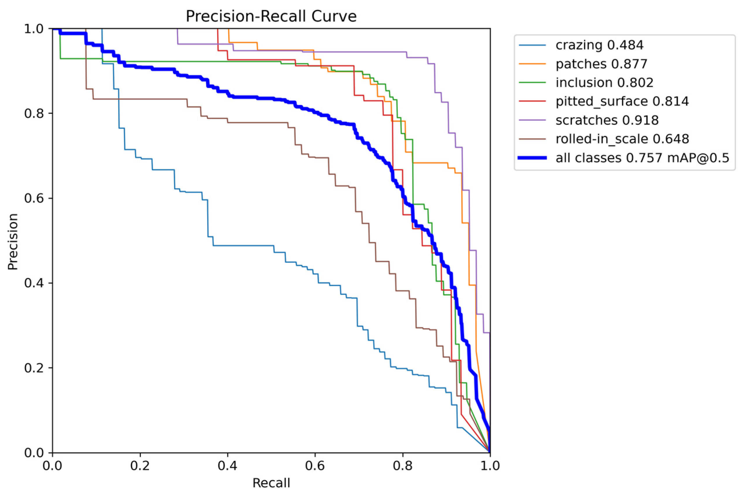
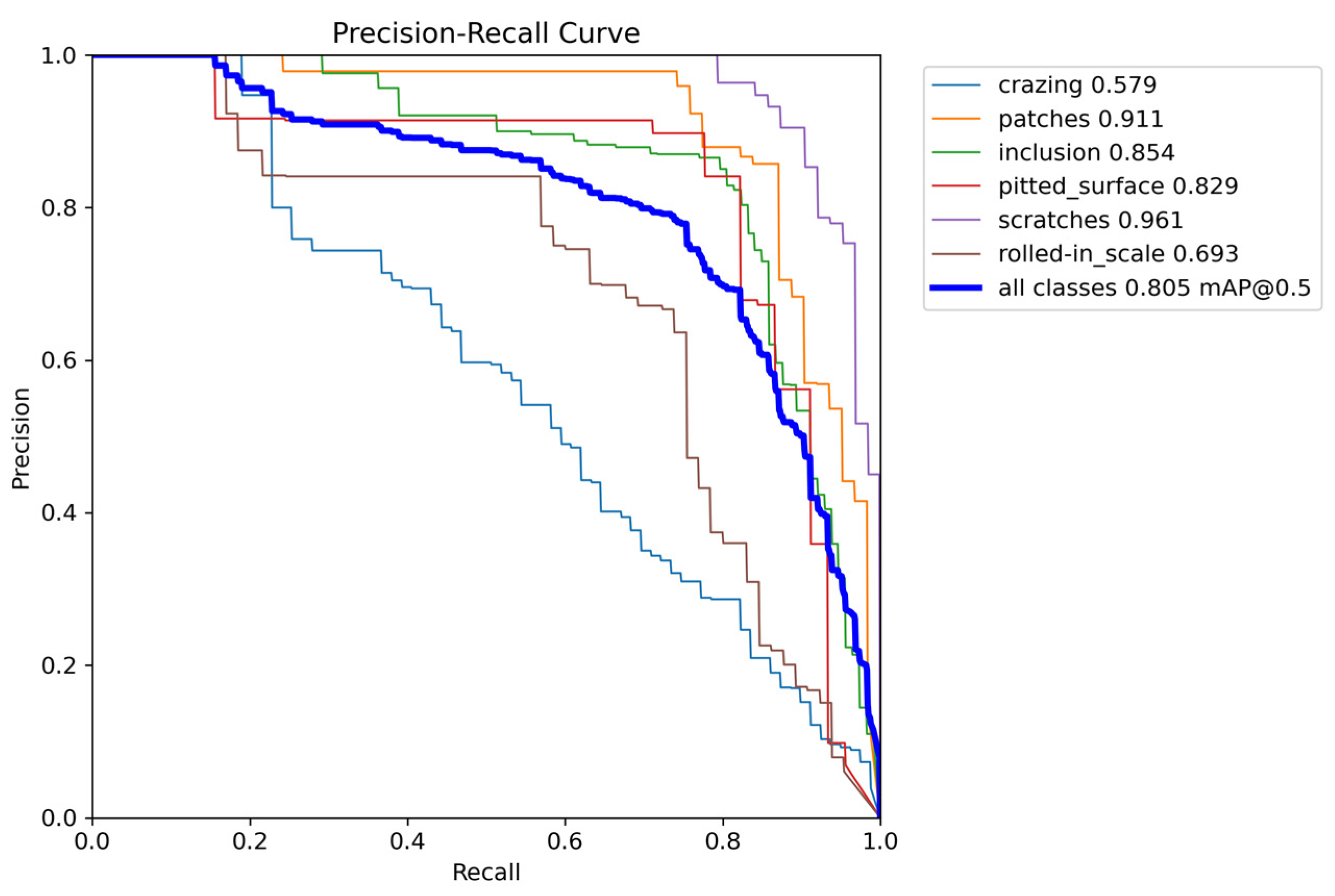
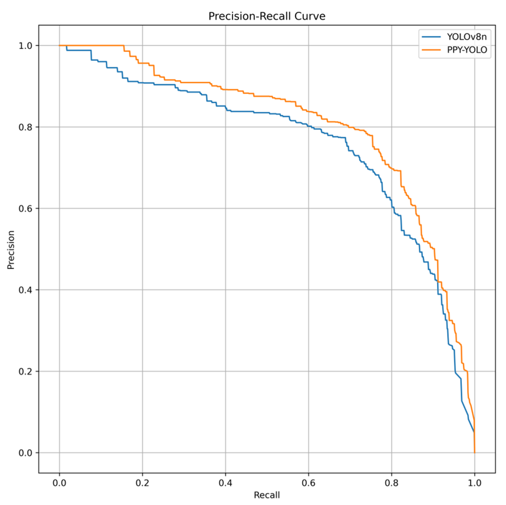
Figure 10 and
Figure 11 present the precision–recall (PR) curves for the baseline YOLOv8n and the improved PPY-YOLO models, respectively. The PR curve intuitively demonstrates the detection performance for each defect category, as well as the trade-off between precision and recall. From the figures, we can see that the PPY-YOLO model achieved an mAP@0.5 of 0.805, a significant improvement over the baseline YOLOv8n’s 0.757. Furthermore, the PR curves for all defect categories, except pitted_surface, show varying degrees of significant improvement, with the AP for the crazing category showing a particularly notable rise. This indicates that the PPY-YOLO model has a significant advantage in overall performance across almost all categories compared to the baseline. Regarding the shape of the PR curves, a curve closer to the top-right corner indicates better model performance. As shown in
Figure 10,
Figure 11 and
Figure 12, a comparison of the curves reveals that both PPY-YOLO’s overall PR curve for all classes and the curves for its individual categories are all closer to the top-right corner than those of the baseline. This shows that PPY-YOLO achieved better performance across the entire precision–recall trade-off. Specifically, the PPY-YOLO PR curves are generally smoother and positioned higher than YOLOv8n’s. This suggests that when precision is sacrificed for higher recall, PPY-YOLO’s performance degradation is slower, highlighting its robustness and stability.
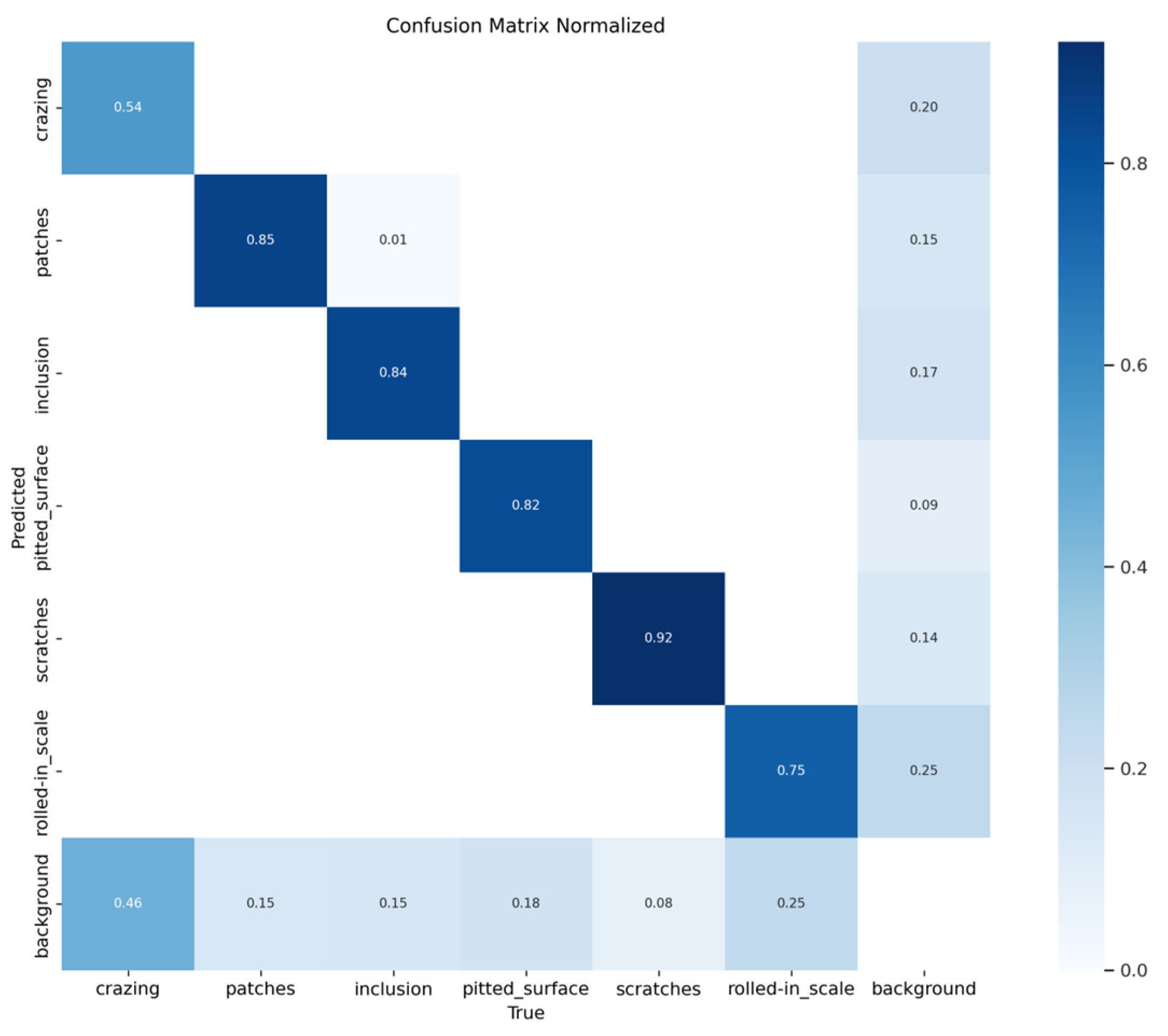
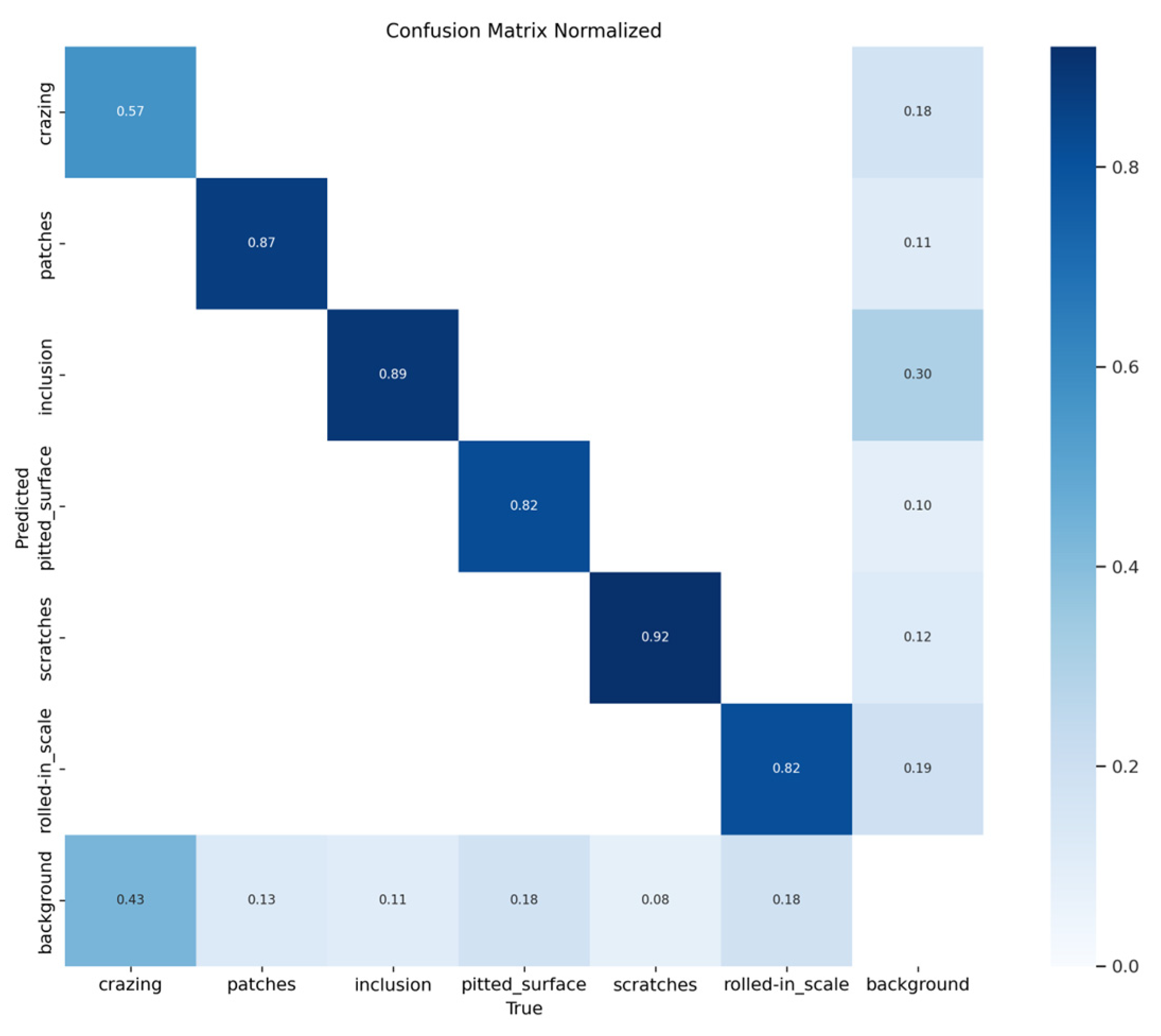
Figure 13 and
Figure 14 present the normalized confusion matrices for the Baseline and PPY-YOLO models, respectively. We can observe that the diagonal values, representing the recall of each category, are either stable or significantly improved. The most notable improvements are seen in the inclusion and rolled-in_scale categories. The recall for inclusion increased from 0.84 to 0.89, while rolled-in_scale saw a substantial jump from 0.75 to 0.82. This demonstrates PPY-YOLO’s enhanced ability to detect these specific defect types more effectively. Furthermore, the recall for the patches and crazing categories also experienced slight increases, from 0.85 to 0.87 and 0.54 to 0.57, respectively. The recall for pitted_surface and scratches remained stable at 0.82 and 0.92, indicating that PPY-YOLO successfully maintains the high performance achieved by the baseline model in these categories. Furthermore, most false positive indicators related to the background class have also decreased. Overall, these results indicate that PPY-YOLO can more precisely distinguish target defects from complex backgrounds.
4.3.3. Comparative Experiment of Attention Mechanism
To verify the validity of the improved GAM-B attention mechanism, we add this attention mechanism to YOLOv8n. We do this on the basis of introducing New-Neck, and place it above all SPPF layers. We conduct a horizontal comparison and analysis of three attention mechanisms: GAM-B, GAM, and CBAM. The results of the attention mechanism comparison experiment are shown in
Table 2.
From
Table 2, we can see that after adding the CBAM attention mechanism to New-Neck-v8n, the mAP@0.5, precision (P) and recall (R) all showed a decrease. However, adding the GAM or GAM-B attention mechanism to New-Neck-v8n increased these metrics.
With the GAM attention mechanism, the mAP@0.5 increased to 77.2%, a 0.9% improvement. Its precision reached 75.9% and recall was 72.6%. The model had 4.6 million parameters and 10.4 GFLOPs. With the GAM-B attention mechanism, the mAP@0.5 increased to 76.5%, a 0.2% improvement. Its precision was 74.4% and recall was 73.0%. The model had 3.0 million parameters and 9.1 GFLOPs. Notably, while the CBAM mechanism led to a decrease in most performance metrics, its mAP@0.5:0.95 of 42.9% was the highest among all compared models. The mAP@0.5:0.95 metric, which measures performance across a stricter range of IoU thresholds, is a strong indicator of a model’s ability to precisely localize a defect’s bounding box. A higher mAP@0.5:0.95 means the model is better at drawing tight, accurate boxes around the defects. However, precision and recall are the foundational metrics for defect detection. A model must first be able to accurately identify and find the defects before it can be judged on the precision of its bounding boxes. The low precision (70.8%) and recall (70.7%) of the CBAM mechanism indicate a significant number of false positives and false negatives, making it unreliable for initial defect screening despite its high bounding box quality.
Based on the data analysis in this section, a comprehensive consideration of all metrics shows that the GAM-B mechanism is the most promising. It can maintain the parameter count and computational cost at a level identical to that of New-Neck-v8n while improving core detection accuracy metrics.
When comparing the GAM-B and GAM attention mechanisms, although the mAP@0.5 and mAP@0.5:0.95 of GAM-B were slightly lower, its recall (73.0%) was actually higher than that of GAM (72.6%). More importantly, to achieve this competitive performance, GAM-B reduced its parameter count by 34.7% and computational cost by 12.5%. This demonstrates GAM-B’s superior efficiency. Also, as shown in
Section 4.3.1, when the baseline incorporates both the New-Neck and C2f_RVB modules, the GAM-B attention mechanism can significantly increase the detection accuracy by 1.8 percentage points. This shows that in the steel surface defect detection scenario, the improved GAM-B attention mechanism has greater practical application value than the original GAM attention mechanism.
4.3.4. Comparative Experiment
We conducted a comparative experiment under the same conditions, evaluating our PPY-YOLO model against several current mainstream object detection algorithms. These algorithms include Faster RCNN, SSD, YOLOv4, YOLOv5s, YOLOv7-tiny, YOLOv8n, YOLOv11n, and models from five references in the literature. The results of this comprehensive comparison are presented in
Table 3.
As shown in
Table 3, The Faster R-CNN algorithm has a high accuracy of 76.9%. However, its detection speed FPS is only 18 frames per second, failing to meet the real-time detection requirements. The detection accuracies of SSD and YOLOv4 are relatively low.
Among the YOLO series, the detection accuracies of YOLOv5s, YOLOv7-tiny, YOLOv8n, and YOLOv11n are all competitive. However, YOLOv5s and YOLOv7-tiny have significantly higher parameter counts and computational costs. YOLOv11n has the lowest parameter count and computational cost, while YOLOv8n achieves a slightly higher mAP@0.5, FPS, and mAP@0.5:0.95. YOLOv8n achieves the best balance between detection accuracy and computational efficiency.
The five referenced models also achieve high accuracy, with Method proposed in [
41] reaching an mAP@0.5 of 81.9% and Egc-yolo method proposed in [
40] reaching 80.2%. However, their parameter counts and GFLOPs are significantly higher than our PPY-YOLO model. For example, the model in Method proposed in [
41] has 38.6 million parameters, which is 18 times that of our model, while Egc-yolo method proposed in [
40] has 3.3 million parameters, which is still 1.5 times that of PPY-YOLO.
Compared to these models, PPY-YOLO demonstrates a superior balance. Its mAP@0.5 of 80.5% and mAP@0.5:0.95 of 45% are the highest among all real-time models and are notably 4.8% higher than the YOLOv8n baseline. While the FPS of PPY-YOLO is slightly lower than that of YOLOv8n, its speed still meets industrial detection standards. Moreover, PPY-YOLO features the minimal parameter count and the lowest computational burden among all compared algorithms, including the referenced models.
In summary, PPY-YOLO performs optimally in the steel surface defect detection scenario. Its lower number of parameters and computational load also offer a new approach for deploying the model to mobile detection devices.
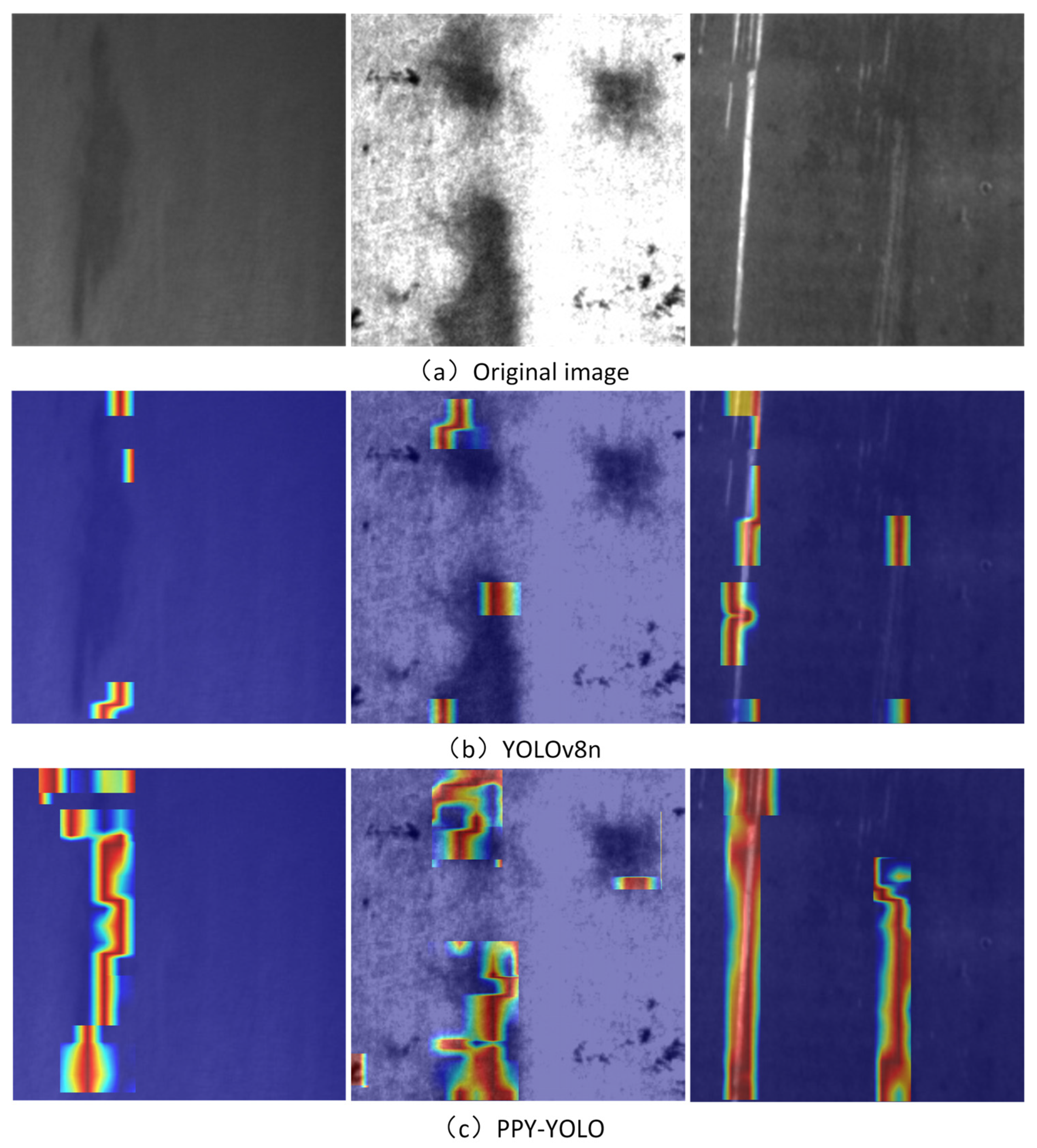
4.3.5. Heatmap Analysis
To further validate the improvement effect of our proposed algorithm, we randomly selected three different types of steel surface defect images from the NEU-DET dataset’s test set. We employed the Grad-CAM method to generate and visualize heatmaps [
44]. This allows for a more intuitive analysis of the regions of focus before and after model improvement.
Figure 15 illustrates the visualization results.
Figure 15 indicates the original YOLOv8n network’s susceptibility to factors like background and lighting. It focuses on targets other than defects.
In contrast, the PPY-YOLO model is more clearly focused on the defect target region. This indicates that the network’s feature extraction ability in the target region has been effectively enhanced. Furthermore, its attention distraction to irrelevant regions has been reduced.
Therefore, PPY-YOLO can help the network further strengthen the model’s perception of local details while grasping the overall context. This significantly improves the detection accuracy and robustness.
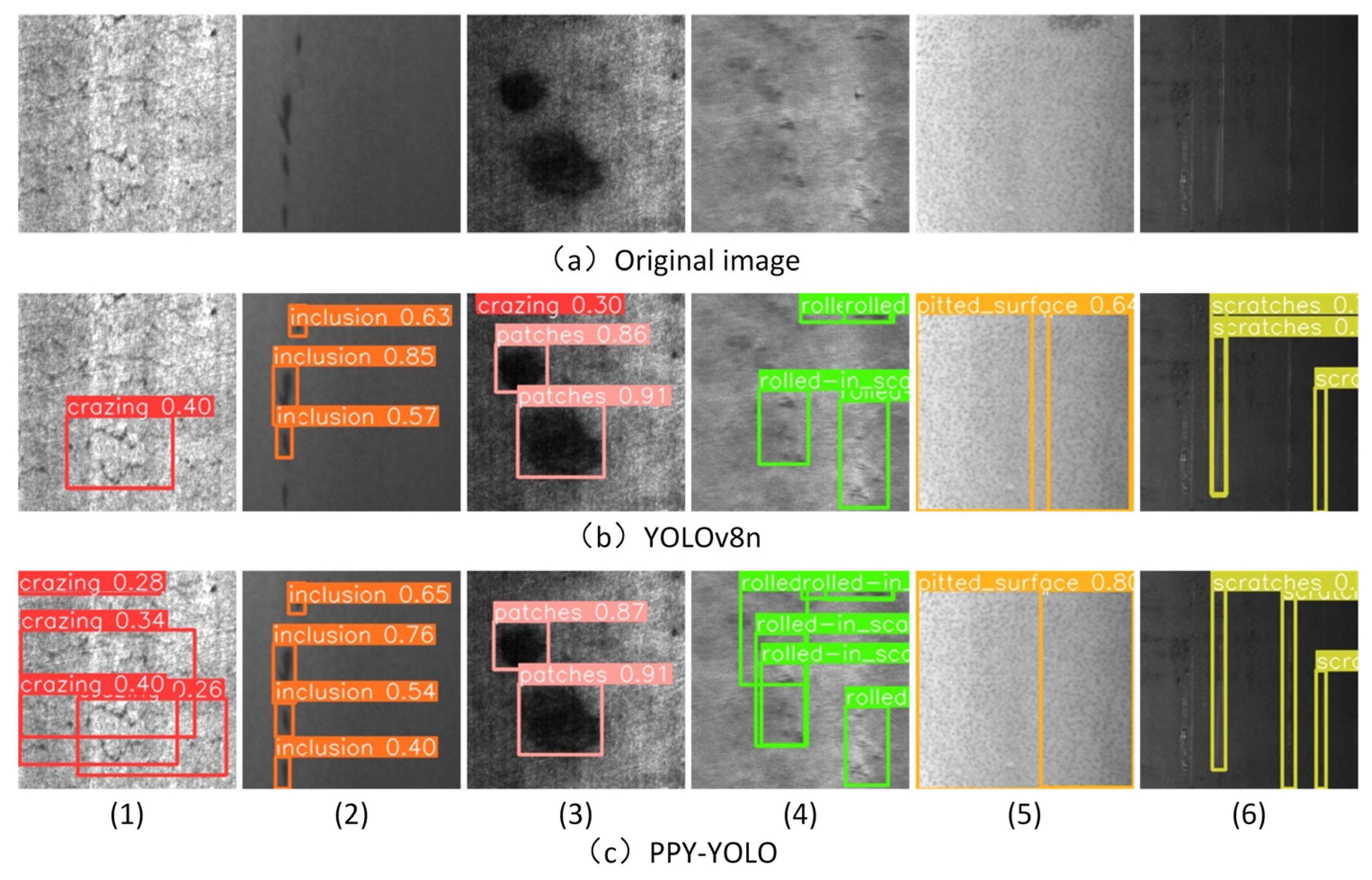
4.3.6. Analysis of Detection Performance
To verify the improvement effect of the model more intuitively, this section compares the detection effects of the two algorithms. We randomly selected images from the NEU-DET dataset’s test set and performed detection using both the YOLOv8n network and the PPY-YOLO model.
Figure 16 displays the detection results from these two algorithms.
The detection results indicate that the improved PPY-YOLO has significantly enhanced the detection accuracy compared to the baseline. Specifically, it has addressed issues in the pre-improvement YOLOv8n model. For example, it has resolved the false detection problem in Result Group (3) and the missed detection issues in Result Groups (1), (2), (4), (5), and (6). Moreover, the confidence of each group of results has also been somewhat improved.
This shows that the improved PPY-YOLO model in this paper has a more outstanding detection ability in the steel surface defect scenario. It can meet the requirements of industrial identification and rapid detection of steel surface defects.
4.3.7. Experiment on Generalization Ability
To verify the generalization ability of our improved algorithm, we use the industrial surface defect dataset GC10-DET for testing. The GC10-DET and NEU-DET datasets have similar properties and are both small-target defect detection datasets.
The GC10-DET dataset contains ten types of surface defects: punched holes (Pu), weld seams (Wl), crescent-shaped gaps (Cg), water spots (Ws), oil spots (Os), thread spots (Ss), inclusions (In), rolling pits (Rp), creases (Cr), and waist creases (Wf). It has 3570 grayscale images, divided into a training set, a validation set, and a test set at an 8:1:1 ratio.
Under the same experimental parameters, configurations, and evaluation metrics as in
Section 3.1 and
Section 3.2, we conduct an experimental comparison using the improved model PPY-YOLO and the baseline YOLOv8n algorithm. The experimental results are shown in
Table 4.
Table 4 clearly shows that the improved model PPY-YOLO proposed in this paper achieved an mAP@0.5 of 69.2 on the GC10-DET dataset. This is 6.6% higher than the baseline. Furthermore, the mAP@0.5:0.95 saw a significant increase from 31.3% to 36.6%. Meanwhile, the number of parameters decreased by 30% and the computational cost dropped by 30.8%. The experimental results verify that the algorithm in this paper has good generalization ability and superior detection performance.
5. Conclusions and Future Work
In this study, we added an upsampling layer and a feature fusion layer to the neck of YOLOv8n. This enhanced its feature extraction and feature fusion abilities. We introduced the C2f_RVB module. It assists the model in concentrating more on the key image information and reduces model complexity. We introduced an improved GAM-B attention mechanism. This allows the network model to focus on the image’s key information in both channel and spatial dimensions. When reconstructing the detection head, we significantly reduced the model complexity and improved the detection accuracy. Experimental results show that the improved algorithm reduces device computing and storage requirements while maintaining accuracy improvements. The model in this paper is more easily deployable on resource-constrained devices.
This study has a primary advantage over existing YOLOv8n improvements: it achieves a better balance between accuracy and deployability. Many current YOLOv8n enhancements focus on maximum accuracy, which causes a large increase in resource consumption. However, in various industrial scenarios and on resource-constrained devices, low-resource models are essential for practical deployment. Our improvements cut the model’s complexity and resource needs, maintaining or even exceeding the accuracy of existing models. Emphasizing both lightweight design and efficiency, our model can perform high-performance detection. It is more suitable for deployment on mobile devices, embedded systems, and other computationally limited environments. This fills a gap in the deployment efficiency of current enhancement efforts.
The algorithm here boosts performance and cuts computational and storage needs. This matters a lot for practical applications. For example, in mobile real-time detection, our model enables smartphones and alike to run complex object detection tasks efficiently and locally. They do not need high-computation cloud resources. This enhances user experience greatly. In embedded systems like robotic vision systems, the model’s lightweight feature allows it to integrate into power and resource-limited hardware platforms. Thus, it is very suitable for real-time industrial inspection. This efficient deployment can reduce hardware costs and energy use. It also paves the way for wider AI adoption in different real-world situations.
However, our study also has several limitations. It should be noted that the model training requires a large-scale annotated dataset and substantial computational resources. The high resource consumption during the training phase remains a key consideration for broader application, especially in environments with limited data or computing power. Furthermore, despite our lightweight design, the inference speed of the model might still be suboptimal for some highly real-time applications, such as on high-speed production lines. And although the model is highly efficient, it still faces challenges in real-world industrial environments. For instance, variable lighting conditions and complex background noise, such as oil stains and reflections on the steel surface, could negatively impact the model’s performance.
Although this study makes remarkable progress in balancing YOLOv8n’s lightweight design and performance, future research offers more opportunities. First, we plan to improve detection precision further. This might mean exploring advanced feature enhancement techniques, optimizing loss function designs or using more efficient training strategies. Second, we will focus on applying and optimizing the model for embedded systems. This includes quantizing, pruning the model, and performing hardware acceleration for different embedded hardware platforms. We aim to get higher inference speeds and lower energy consumption. Also, we need to ensure the model is robust and stable in real industrial settings.
6. Patents
Zhao, J.; Peng, Y.; Zhang, S.; Liu, S.; Duan, J.; Huang, X.; Yin, Z. A Steel Surface Defect Detection Method and System Based on PPY-YOLO. Chinese Patent CN119672031B, 25 April 2025.
Author Contributions
J.Z. and S.Z. are first co-authors of the article. Conceptualization, J.Z. and S.Z.; methodology, J.Z. and S.Z.; software, Y.P.; validation, Y.P. and S.Z.; formal analysis, S.Z. and X.L.; investigation, J.Z.; resources, Y.P.; data curation, Y.P. and S.Z.; writing—original draft preparation, Y.P. and S.Z.; writing—review and editing, J.Z. and X.L.; visualization, S.Z.; supervision, J.Z. and X.L.; project administration, J.Z.; funding acquisition, J.Z. and X.L. All authors have read and agreed to the published version of the manuscript.
Funding
This research was funded by the Key Research and Development Program of Hunan Province under grant NO. 2024JK2007; Hunan Provincial Natural Science Foundation of China under grant No. 2023JJ40237; Guangxi Science and Technology Major Program under grant No. 2024AA15007.
Data Availability Statement
The original contributions presented in this study are included in the article. Further inquiries can be directed to the corresponding author.
Conflicts of Interest
The authors declare no conflicts of interest.
Abbreviations
The following abbreviations are used in this manuscript:
| PPY | Performance-enhanced, Parameter-efficient, Young |
| YOLO | You Only Look Once |
| GAM | Global Attention Module |
| C2f_RVB | CSP Bottleneck with 2 Convolutions RepViT Block |
| DWConv | Depthwise Convolutions |
| BatchNorm | Batch Normalization |
References
- Yin, Q. Design and Application of Smart City Internet of Things Service Platform Based on Fuzzy Clustering Algorithm. Mob. Inf. Syst. 2022, 2022, 8405306. [Google Scholar] [CrossRef]
- Zhang, P.; Zhu, H.; Li, W.; Alfarraj, O.; Tolba, A.; Kim, G.-J. Secure and Efficient Data Transmission Scheme Based on Physical Mechanism. Comput. Mater. Contin. 2023, 75, 3589–3605. [Google Scholar] [CrossRef]
- Zhou, X.; Xu, X.; Liang, W.; Zeng, Z.; Yan, Z. Deep-Learning-Enhanced Multitarget Detection for End–Edge–Cloud Surveillance in Smart IoT. IEEE Internet Things J. 2021, 8, 12588–12596. [Google Scholar] [CrossRef]
- Wu, M.; Wu, Y.; Liu, X.; Ma, M.; Liu, A.; Zhao, M. Learning-Based Synchronous Approach from Forwarding Nodes to Reduce the Delay for Industrial Internet of Things. EURASIP J. Wirel. Commun. Netw. 2018, 2018, 10. [Google Scholar] [CrossRef]
- Zhang, J.; Alam Bhuiyan, Z.; Yang, X.; Wang, T.; Xu, X.; Hayajneh, T.; Khan, F. AntiConcealer: Reliable Detection of Adversary Concealed Behaviors in EdgeAI-Assisted IoT. IEEE Internet Things J. 2021, 9, 22184–22193. [Google Scholar] [CrossRef]
- Zhang, D.; Qiao, Y.; She, L.; Shen, R.; Ren, J.; Zhang, Y. Two Time-Scale Resource Management for Green Internet of Things Networks. IEEE Internet Things J. 2018, 6, 545–556. [Google Scholar] [CrossRef]
- Zhao, J.; Hosseini, S.; Chen, Q.; Armaghani, D.J. Super Learner Ensemble Model: A Novel Approach for Predicting Monthly Copper Price in Future. Resour. Policy 2023, 85, 103903. [Google Scholar] [CrossRef]
- Deshpande, A.M.; Minai, A.A.; Kumar, M. One-Shot Recognition of Manufacturing Defects in Steel Surfaces. Procedia Manuf. 2020, 48, 1064–1071. [Google Scholar] [CrossRef]
- Mo, C.; Sun, W. Point-by-Point Feature Extraction of Artificial Intelligence Images Based on the Internet of Things. Comput. Commun. 2020, 159, 1–8. [Google Scholar] [CrossRef]
- Zhou, X.; Liang, W.; Wang, K.I.-K.; Wang, H.; Yang, L.T.; Jin, Q. Deep-Learning-Enhanced Human Activity Recognition for Internet of Healthcare Things. IEEE Internet Things J. 2020, 7, 6429–6438. [Google Scholar] [CrossRef]
- Jiang, W.; Lv, S. Hierarchical Deployment of Deep Neural Networks Based on Fog Computing Inferred Acceleration Model. Clust. Comput. 2021, 24, 2807–2817. [Google Scholar] [CrossRef]
- Kong, X.; Li, J. Vision-Based Fatigue Crack Detection of Steel Structures Using Video Feature Tracking. Comput. Aided Civ. Infrastruct. Eng. 2018, 33, 783–799. [Google Scholar] [CrossRef]
- Leng, Y.; Liu, Z.; Xu, B.; Li, Z. Improved Faster R-CNN for Surface Defect Detection of Steel. Mach. Sci. Technol. 2025, 44, 75–83. [Google Scholar] [CrossRef]
- Kou, X.; Liu, S.; Cheng, K.; Qian, Y. Development of a YOLO-V3-based Model for Detecting Defects on Steel Strip Surface. Measurement 2021, 182, 109454. [Google Scholar] [CrossRef]
- Zhao, C.; Shu, X.; Yan, X.; Zuo, X.; Zhu, F. RDD-YOLO: A Modified YOLO for Detection of Steel Surface Defects. Measurement 2023, 214, 112776. [Google Scholar] [CrossRef]
- Wang, M.; Liu, Z. Improved YOLOv8 Algorithm for Steel Surface Defect Detection. Mach. Sci. Technol. 2025, 44, 19–29. [Google Scholar] [CrossRef]
- Cui, K.; Jiao, J. Steel Surface Defect Detection Algorithm Based on MCB-FAH-YOLOv8. J. Graph. 2024, 45, 112–125. [Google Scholar] [CrossRef]
- Song, X.; Cao, S.; Zhang, J.; Hou, Z. Steel Surface Defect Detection Algorithm Based on YOLOv8. Electronics 2024, 13, 988. [Google Scholar] [CrossRef]
- Peng, X.; Ren, J.; She, L.; Zhang, D.; Li, J.; Zhang, Y. BOAT: A Block-Streaming App Execution Scheme for Lightweight IoT Devices. IEEE Internet Things J. 2018, 5, 1816–1829. [Google Scholar] [CrossRef]
- Zhou, X.; Wu, J.; Liang, W.; Wang, K.I.-K.; Yan, Z.; Yang, L.T.; Jin, Q. Reconstructed Graph Neural Network with Knowledge Distillation for Lightweight Anomaly Detection. IEEE Trans. Neural Netw. Learn. Syst. 2024, 35, 11817–11828. [Google Scholar] [CrossRef] [PubMed]
- Tong, Y.; Sun, W. The Role of Film and Television Big Data in Real-Time Image Detection and Processing in the Internet of Things Era. J. Real-Time Image Process. 2021, 18, 1115–1127. [Google Scholar] [CrossRef]
- Zhou, X.; Liang, W.; Yan, K.; Li, W.; Wang, K.I.-K.; Ma, J.; Jin, Q. Edge-Enabled Two-Stage Scheduling Based on Deep Reinforcement Learning for Internet of Everything. IEEE Internet Things J. 2022, 10, 3295–3304. [Google Scholar] [CrossRef]
- Liu, J.; Zhang, X. Truthful Resource Trading for Dependent Task Offloading in Heterogeneous Edge Computing. Future Gener. Comput. Syst. 2022, 133, 228–239. [Google Scholar] [CrossRef]
- Lin, T.Y.; Dollár, P.; Girshick, R.; He, K.; Hariharan, B.; Belongie, S. Feature Pyramid Networks for Object Detection. In Proceedings of the IEEE Conference on Computer Vision and Pattern Recognition (CVPR), Honolulu, HI, USA, 21–26 July 2017; pp. 2117–2125. [Google Scholar] [CrossRef]
- Ruiz-Ponce, P.; Ortiz-Perez, D.; Garcia-Rodriguez, J.; Kiefer, B. Poseidon: A Data Augmentation Tool for Small Object Detection Datasets in Maritime Environments. Sensors 2023, 23, 3691. [Google Scholar] [CrossRef] [PubMed]
- Wang, C.Y.; Bochkovskiy, A.; Liao, H.Y.M. YOLOv7: Trainable Bag-of-Freebies Sets New State-of-the-Art for Real-Time Object Detectors. In Proceedings of the IEEE/CVF Conference on Computer Vision and Pattern Recognition (CVPR), Vancouver, BC, Canada, 17–24 June 2023; pp. 7464–7475. [Google Scholar] [CrossRef]
- Liu, Y.; Shao, Z.; Hoffmann, N. Global Attention Mechanism: Retain Information to Enhance Channel-Spatial Interactions. arXiv 2021, arXiv:2112.05561. [Google Scholar] [CrossRef]
- Woo, S.; Park, J.; Lee, J.-Y.; Kweon, I.S. CBAM: Convolutional Block Attention Module. In Proceedings of the Computer Vision—ECCV 2018: 15th European Conference, Munich, Germany, 8–14 September 2018; Part VII. pp. 3–19. [Google Scholar] [CrossRef]
- Wang, J.; Lv, P.; Wang, H.; Shi, C. SAR-U-Net: Squeeze-and-Excitation Block and Atrous Spatial Pyramid Pooling Based Residual U-Net for Automatic Liver Segmentation in Computed Tomography. Comput. Methods Programs Biomed. 2021, 208, 106268. [Google Scholar] [CrossRef] [PubMed]
- Tolstikhin, I.O.; Houlsby, N.; Kolesnikov, A.; Beyer, L.; Zhai, X.; Unterthiner, T.; Yung, J.; Steiner, A.; Keysers, D.; Uszkoreit, J.; et al. MLP-Mixer: An All-MLP Architecture for Vision. In Proceedings of the Advances in Neural Information Processing Systems 34 (NeurIPS 2021), Virtual, 6–14 December 2021; pp. 24261–24272. [Google Scholar] [CrossRef]
- Li, Y.; Hou, Q.; Zheng, Z.; Cheng, M.-M.; Yang, J.; Li, X. Large selective kernel network for remote sensing object detection. In Proceedings of the IEEE/CVF International Conference on Computer Vision, Paris, France, 1–6 October 2023; pp. 16794–16805. [Google Scholar] [CrossRef]
- He, J.; Wang, Y.; Wang, Y.; Li, R.; Zhang, D.; Zheng, Z. A Lightweight Road Crack Detection Algorithm Based on Improved YOLOv7 Model. Signal Image Video Process. 2024, 18 (Suppl S1), 847–860. [Google Scholar] [CrossRef]
- Wang, A.; Chen, H.; Lin, Z.; Han, J.; Ding, G. Rep ViT: Revisiting Mobile CNN From ViT Perspective. In Proceedings of the 2024 IEEE/CVF Conference on Computer Vision and Pattern Recognition (CVPR), Seattle, WA, USA, 16–22 June 2024; pp. 15909–15920. [Google Scholar] [CrossRef]
- Koonce, B. MobileNetv3. In Convolutional Neural Networks with Swift for TensorFlow: Image Recognition and Dataset Categorization; Apress: New York, NY, USA, 2021; pp. 125–144. [Google Scholar] [CrossRef]
- Tan, M.; Chen, B.; Pang, R.; Vasudevan, V.; Sandler, M.; Howard, A.; Le, Q.V. Mnasnet: Platform-Aware Neural Architecture Search for Mobile. In Proceedings of the 2019 IEEE/CVF Conference on Computer Vision and Pattern Recognition (CVPR), Long Beach, CA, USA, 15–20 June 2019; pp. 2820–2828. [Google Scholar] [CrossRef]
- He, Y.; Song, K.; Meng, Q.; Yan, Y. An End-to-End Steel Surface Defect Detection Approach via Fusing Multiple Hierarchical Features. IEEE Trans. Instrum. Meas. 2019, 69, 1493–1504. [Google Scholar] [CrossRef]
- Ren, S.; He, K.; Girshick, R.; Sun, J. Faster R-CNN: Towards Real-Time Object Detection with Region Proposal Networks. IEEE Trans. Pattern Anal. Mach. Intell. 2016, 39, 1137–1149. [Google Scholar] [CrossRef]
- Liu, W.; Anguelov, D.; Erhan, D.; Szegedy, C.; Reed, S.; Fu, C.Y.; Berg, A.C. SSD: Single Shot MultiBox Detector. In Proceedings of the Computer Vision—ECCV 2016: 14th European Conference, Amsterdam, The Netherlands, 11–14 October 2016; Part I. Springer International Publishing: Cham, Switzerland, 2016; pp. 21–37. [Google Scholar] [CrossRef]
- Liang, L.; Chen, K.; Chen, L.; Long, P. Improving the lightweight FCM-YOLOv8n for steel surface defect detection. Opto-Electron. Eng. 2025, 52, 240280. [Google Scholar] [CrossRef]
- Ni, Y.; Zi, D.; Chen, W.; Wang, S.; Xue, X. Egc-yolo: Strip steel surface defect detection method based on edge detail enhancement and multiscale feature fusion. J. Real-Time Image Process. 2025, 22, 65. [Google Scholar] [CrossRef]
- Wang, Y.; Wang, H.; Xin, Z. Efficient detection model of steel strip surface defects based on YOLO-V7. IEEE Access 2022, 10, 133936–133944. [Google Scholar] [CrossRef]
- Xu, K.; Zhu, D.; Shi, C.; Zhou, C. YOLO-DBL: A multi-dimensional optimized model for detecting surface defects in steel. J. Membr. Comput. 2025, 1–11. [Google Scholar] [CrossRef]
- Li, H.; Zhang, H.; Zang, W. StripSurface-YOLO: An Enhanced Yolov8n-Based Framework for Detecting Surface Defects on Strip Steel in Industrial Environments. Electronics 2025, 14, 2994. [Google Scholar] [CrossRef]
- Selvaraju, R.R.; Cogswell, M.; Das, A.; Vedantam, R.; Parikh, D.; Batra, D. Grad-CAM: Visual Explanations From Deep Networks via Gradient-Based Localization. In Proceedings of the IEEE International Conference on Computer Vision (ICCV), Venice, Italy, 22–29 October 2017; pp. 618–626. [Google Scholar] [CrossRef]
Figure 1.
Detailed architecture diagram of the YOLOv8 network.
Figure 1.
Detailed architecture diagram of the YOLOv8 network.
Figure 2.
The architecture diagram of the PPY-YOLO model.
Figure 2.
The architecture diagram of the PPY-YOLO model.
Figure 3.
A new path graph has been added to the neck structure.
Figure 3.
A new path graph has been added to the neck structure.
Figure 4.
The structure graph of GAM attention mechanism.
Figure 4.
The structure graph of GAM attention mechanism.
Figure 5.
Structure diagram of the DWConv group.
Figure 5.
Structure diagram of the DWConv group.
Figure 6.
Structure of the GAM-B attention mechanism.
Figure 6.
Structure of the GAM-B attention mechanism.
Figure 7.
Structural diagram of the C2f-RVB module.
Figure 7.
Structural diagram of the C2f-RVB module.
Figure 8.
Reconstruction of the structural diagram of the detection head. (a) Presents the original detection head. (b) Shows the improved detection head proposed herein.
Figure 8.
Reconstruction of the structural diagram of the detection head. (a) Presents the original detection head. (b) Shows the improved detection head proposed herein.
Figure 9.
Example of images from the database across all categories of defects.
Figure 9.
Example of images from the database across all categories of defects.
Figure 10.
PR curve of YOLOv8n.
Figure 10.
PR curve of YOLOv8n.
Figure 11.
PR curve of PPY-YOLO.
Figure 11.
PR curve of PPY-YOLO.
Figure 12.
The PR curve comparison of PPY-YOLO and YOLOv8n for all classes.
Figure 12.
The PR curve comparison of PPY-YOLO and YOLOv8n for all classes.
Figure 13.
Normalized confusion matrix of YOLOv8n.
Figure 13.
Normalized confusion matrix of YOLOv8n.
Figure 14.
Normalized confusion matrix of PPY-YOLO.
Figure 14.
Normalized confusion matrix of PPY-YOLO.
Figure 15.
Heatmap visualization outcomes. (a) Presents the original image, (b) shows the detection performance of the baseline model YOLOv8n, and (c) demonstrates the detection performance of the model proposed in this paper.
Figure 15.
Heatmap visualization outcomes. (a) Presents the original image, (b) shows the detection performance of the baseline model YOLOv8n, and (c) demonstrates the detection performance of the model proposed in this paper.
Figure 16.
Detection performance. (a) Represents the original input image. (b) Shows the detection results of the baseline YOLOv8n model. (c) Presents the detection results of the model proposed in this paper. Sub-graphs (1–6), respectively, correspond to instance images of different defect classes randomly chosen from the test set.
Table 1.
Ablation experiment result on the NEU-DET dataset.
Table 1.
Ablation experiment result on the NEU-DET dataset.
| New-Neck | C2f_RVB | GAM-B | New-Head | P/% | R/% | mAP@0.5/% | mAP@0.5:0.95 | Params/106 | GFLOPs |
|---|
| | | | | 73.5 | 70.8 | 75.7 | 43.3 | 3.0 | 8.1 |
| √ | | | | 73.9 | 72.1 | 76.3 | 42.3 | 3.0 | 9.1 |
| | √ | | | 74.4 | 68.7 | 75.7 | 42.7 | 2.6 | 7.4 |
| √ | | √ | | 74.4 | 73 | 76.5 | 42.1 | 3.0 | 9.1 |
| | | | √ | 76.9 | 73.9 | 78.8 | 44 | 2.4 | 5.6 |
| √ | √ | | | 75.5 | 73.7 | 78.2 | 43.4 | 2.6 | 8.0 |
| √ | √ | √ | | 74.6 | 74.8 | 80.0 | 44.7 | 2.7 | 8.1 |
| √ | √ | √ | √ | 79.7 | 74.4 | 80.5 | 45 | 2.1 | 5.6 |
Table 2.
Comparison of attention mechanisms on NEU-DET dataset.
Table 2.
Comparison of attention mechanisms on NEU-DET dataset.
| Algorithm | P/% | R/% | mAP@0.5/% | mAP@0.5:0.95 | Params/106 | GFLOPs |
|---|
| New-Neck-v8n | 73.9 | 72.1 | 76.3 | 42.3 | 3.0 | 9.1 |
| GAM-B | 74.4 | 73 | 76.5 | 42.1 | 3.0 | 9.1 |
| GAM | 75.9 | 72.6 | 77.2 | 42.5 | 4.6 | 10.4 |
| CBAM | 70.8 | 70.7 | 75.9 | 42.9 | 3.1 | 9.1 |
Table 3.
Comparative experiment results on the NEU-DET dataset.
Table 3.
Comparative experiment results on the NEU-DET dataset.
| Algorithm | mAP@0.5/% | mAP@0.5:0.95 | Params/106 | GFLOPs | FPS |
|---|
| Faster R-CNN [37] | 76.9 | 37.4 | 137.0 | 370.2 | 18 |
| SSD [38] | 69.2 | 30.8 | 26.2 | 62.7 | 46 |
| YOLOv4 | 65.1 | 27.9 | 64.4 | 60.5 | 58 |
| YOLOv5s | 75.1 | 40.6 | 7.0 | 15.8 | 108 |
| YOLOv7-tiny | 75.6 | 40.8 | 6.0 | 13.1 | 57 |
| YOLOv8n | 75.7 | 43.3 | 3.0 | 8.1 | 101 |
| YOLOv11n | 75.6 | 40.6 | 2.5 | 6.3 | 75 |
| PPY-YOLO | 80.5 | 45 | 2.1 | 5.6 | 80 |
| FCM-YOLOv8n method proposed in [39] | 76.7 | - | 2.5 | 6.6 | 154 |
| Egc-yolo method proposed in [40] | 80.2 | - | 3.3 | 8.3 | 136 |
| Method proposed in [41] | 81.9 | - | 38.6 | - | 56 |
| YOLO-DBL method proposed in [42] | 78.0 | - | 2.6 | 6.9 | 129 |
| StripSurface-YOLO method proposed in [43] | 78.1 | 43.8 | 2.3 | 6.0 | - |
Table 4.
Generalization study results on the GC10-DET dataset.
Table 4.
Generalization study results on the GC10-DET dataset.
| Algorithm | mAP@0.5/% | mAP@0.5:0.95 | Params/106 | GFLOPs |
|---|
| YOLOv8n | 62.6 | 31.3 | 3.0 | 8.1 |
| PPY-YOLO | 69.2 | 36.6 | 2.1 | 5.6 |
| Disclaimer/Publisher’s Note: The statements, opinions and data contained in all publications are solely those of the individual author(s) and contributor(s) and not of MDPI and/or the editor(s). MDPI and/or the editor(s) disclaim responsibility for any injury to people or property resulting from any ideas, methods, instructions or products referred to in the content. |
© 2025 by the authors. Licensee MDPI, Basel, Switzerland. This article is an open access article distributed under the terms and conditions of the Creative Commons Attribution (CC BY) license (https://creativecommons.org/licenses/by/4.0/).
