Recurrent Neural Networks (LSTM and GRU) in the Prediction of Current–Voltage Characteristics Curves of Polycrystalline Solar Cells

Abstract

The current–voltage (I-V) characteristic provides essential performance parameters of a solar cell, influenced by temperature and solar radiation. The efficiency of a solar cell is sensitive to variations in these conditions. This study electrically characterized a polycrystalline silicon solar cell in a solar simulator chamber at temperatures of 25–55 °C and irradiance levels of 600–1000 W/m². The acquired data were used to train and evaluate neural network models to predict the I-V characteristics of a polycrystalline silicon solar cell. Two recurrent neural network architectures were tested: LSTM and the GRU model. The performance of the model was assessed using MAE, RMSE, and R². The GRU model achieved the results, with MAE = $2.813\times {10}^{-3}$, RMSE = $5.790\times {10}^{-3}$, and R² = 0.9844, similar to LSTM (MAE = $2.6613\times {10}^{-3}$, RMSE = $5.858\times {10}^{-3}$, R² = 0.9840). These findings highlight the GRU network as the most efficient approach for modeling solar cell behavior under varying environmental conditions.

1. Introduction

Renewable energy is an alternative to traditional power plants [1,2,3,4,5]. In recent times, more specifically in the last century, renewable power has earned recognition over conventional power production [6]. One of the main advantages of solar photovoltaic power plants is their distributed generation [7]. In addition to solar photovoltaic energy generation [2,3,8], there are some other ways of harvesting solar energy, such as solar thermal energy generation, solar thermal water collection, and photocatalysis activated by sunlight, among others [7,9].

The I-V characteristic is required in experiments for the characterization of solar cells [10,11]. This curve allows easy access to various performance parameters, such as fill factor and maximum power point, among others [10,11]. The I-V characteristics must be carefully and accurately measured since it is crucial to be able to distinguish cells correctly in terms of their efficiency [10]. For assessing the I-V parameters precisely, it is necessary to measure different conditions. The main and more relevant conditions are the associated irradiance and temperature [12].

The I-V characteristic of a solar cell represents the electrical response of the device under illumination. It illustrates how the output current varies with the applied voltage and is essential for understanding the cell’s performance. At one end of the curve (short-circuit condition), the voltage is zero and the current reaches its maximum value, defined as the short-circuit current ($I_{SC}$). At the other end (open-circuit condition), the current is zero and the voltage reaches its maximum value, known as the open-circuit voltage ($V_{OC}$) [13].

The shape of the I-V curve is governed by fundamental physical mechanisms, including the photogenerated current, diode ideality, and the internal resistances of the device (series and shunt) [10,11]. From this curve, key performance parameters can be extracted, such as the fill factor ($FF$), the maximum power point ($P_{MPP}$), and the overall energy conversion efficiency [14]. These parameters are highly sensitive to environmental conditions such as temperature and irradiance, making the I-V curve an indispensable tool for characterizing the real-world behavior of photovoltaic devices [15].

The $I_{SC}$ is the current delivered when the voltage across the terminals is zero, and it is directly influenced by the incident irradiance. The $V_{OC}$ is the voltage when no current flows through the external circuit ($I=0$), and it depends primarily on the material properties and temperature of the cell.

The $P_{MPP}$ corresponds to the point on the I-V curve where the product of current and voltage is maximized, representing the operating condition at which the solar cell delivers its highest power output [2,14].

The $FF$ is a dimensionless figure of merit that indicates the “squareness” of the I-V curve. It is defined as the ratio between the actual maximum power and the theoretical power, which would be obtained if the device operated simultaneously at $V_{OC}$ and $I_{SC}$ [13]. The $FF$ is calculated as:

$$FF={\displaystyle \frac{P_{MPP}}{V_{OC}·I_{SC}}}$$

(1)

A higher $FF$ indicates lower internal losses and better overall device quality. Together, $I_{SC}$, $V_{OC}$, $P_{MPP}$, and $FF$ are fundamental parameters for evaluating the efficiency and performance of photovoltaic technologies.

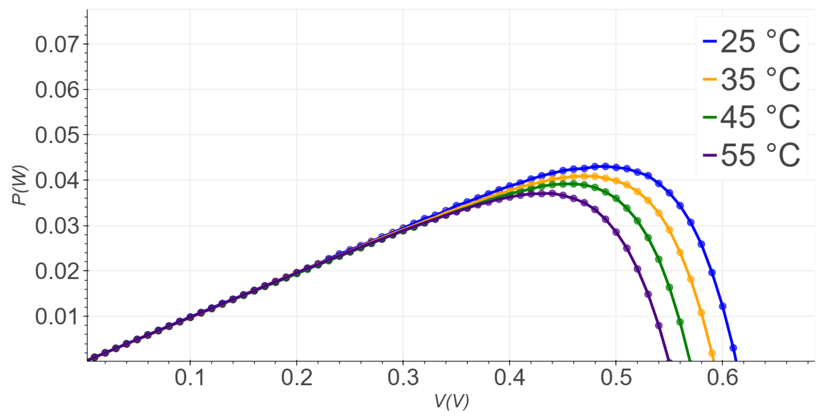
In general, the solar panel manufacturing industry uses specific test conditions, namely standard test conditions (STCs), which correspond to an irradiance of 1000 W/m² and cell temperature of 25 °C [15]. However, corresponding to optimal ratings does not allow us to infer how a cell will perform under varying environmental conditions, as there may be many factors that interfere with the irradiance and temperature conditions [16]. For instance, Figure 1 illustrates the dependence of power on temperature at constant illumination.

The power–voltage (P-V) curve is calculated using the I-V curve; therefore, each point of the I-V curve (these being a pair of voltage and current values) is used in Equation (2) to find the power, where the variable V is the voltage and I is the current. The result is shown in Figure 1.

$$P=V·I$$

(2)

To infer the impact on solar cell performance and to obtain reliable parameters that define its I-V model, it is necessary to apply a method for generating this curve in different scenarios of temperature and irradiance [16,17]. There are some available mathematical models in the literature that can describe this curve [18,19]. The main challenge of these models is the existence of transcendent variables, such as in the single diode model represented by Equation (3), that make it difficult to determine its parameters. The parameters, $I_{ph}$, $I_0$, $Rs$, $R_{sh}$ and n, associated with the cell construction or operating condition, demand intense computational resources due to the equation for the single diode model being transcendental and nonlinear [17,18,20,21].

$$I=I_{ph}-I_0\left[exp\left({\displaystyle \frac{q(V+I{R}_s)}{nkT}}\right)-1\right]-{\displaystyle \frac{V+I{R}_s}{R_{sh}}}$$

(3)

In this equation, I stands for the current (A) between solar cell terminals, $I_{ph}$ for the photocurrent (A), $I_0$ for the diode reverse saturation current (A), q is a constant, the elementary charge, V stands for the voltage through the solar cell terminals, $R_s$ for the series resistance, $R_{sh}$ for the shunt resistance, n for the diode ideality factor, k is the Boltzmann constant, and T is the absolute temperature.

There are three main steps for obtaining these parameters: selection of appropriate equivalent models, mathematical model formulation, and accurate extraction of parameter values from the models [9].

The main environmental conditions that affect solar cell behavior are temperature and illumination. For this reason, there is a need to estimate the solar cell parameters of the single diode model for each temperature and illumination value associated with the respective I-V characteristic curve [22,23]. Due to issues related to accuracy and computational cost, there are many methods for modeling the I-V characteristic curve, and numerous studies have been conducted with the objective of developing new methods of modeling this curve [23,24]. For instance, most approaches consider artificial networks, genetic algorithms, neuro-fuzzy inference systems, and particle swarm optimization [24,25].

Table 1. Typical trends of single-diode parameters with temperature and irradiance.

Parameter	Temperature Effect	Irradiance Effect
$I_{ph}$	slight positive (∼+0.05–0.09%/°C)	linear increase
$I_0$	strong exponential increase	negligible
n	minor increase	negligible
$R_s$	moderate increase	slight increase
$R_{sh}$	decreases	weakly decreases

presents the typical trends of single-diode parameters with temperature and irradiance.

These trends are consistent with both theory and measurement. The $I_{ph}$ increases nearly linearly with irradiance and slightly with temperature, due to temperature-induced increases in thermal carrier generation [26]. The $I_0$ has an exponential dependence on temperature stemming from the diode equation energy gap relation [27]. Parasitic resistances also vary: $R_s$ increases with temperature (higher resistivity) and marginally with irradiance, while $R_{sh}$ decreases under higher thermal loading, indicative of leakage pathways [28]. The n shows minimal irradiance dependence but may increase slightly with temperature, reflecting changes in recombination mechanisms [26].

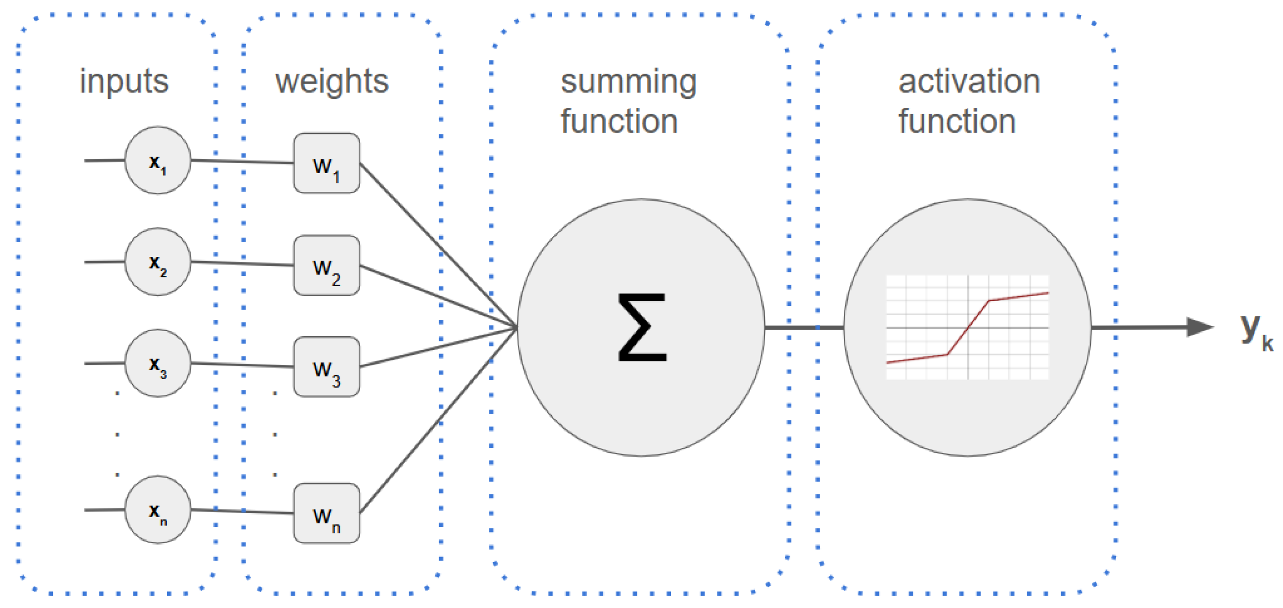
The issue of optimization was developed in the 1940s with the Simplex method was developed. This method was first developed with the objective of solving problem-type linear optimization [29]. In the late 1980s, neural networks became the main method used in machine learning and artificial intelligence [30]. The first generation of neural networks was based on two types called the multilayer perceptron and self-organizing maps. The multilayer perceptron was built with several “nodes” or “artificial neurons”. An illustration of an artificial neural network used in the multilayer perceptron is shown in Figure 2. The multilayer perceptron combines several of these neurons to solve problems (a combination of several neurons is called a network) [30]. These networks learn through a process called backpropagation, in which they adjust their own parameters based on the mistakes they make, improving with each attempt. The second type, self-organizing maps, are networks capable of learning on their own to identify patterns and organize information without receiving direct instructions about what is right or wrong.

Artificial neural networks (ANNs) are computational models inspired by the structure of the human brain capable of solving complex problems involving nonlinear relationships [31]. In the context of solar cells, ANNs have been successfully applied to predict electrical behavior based on environmental variables.

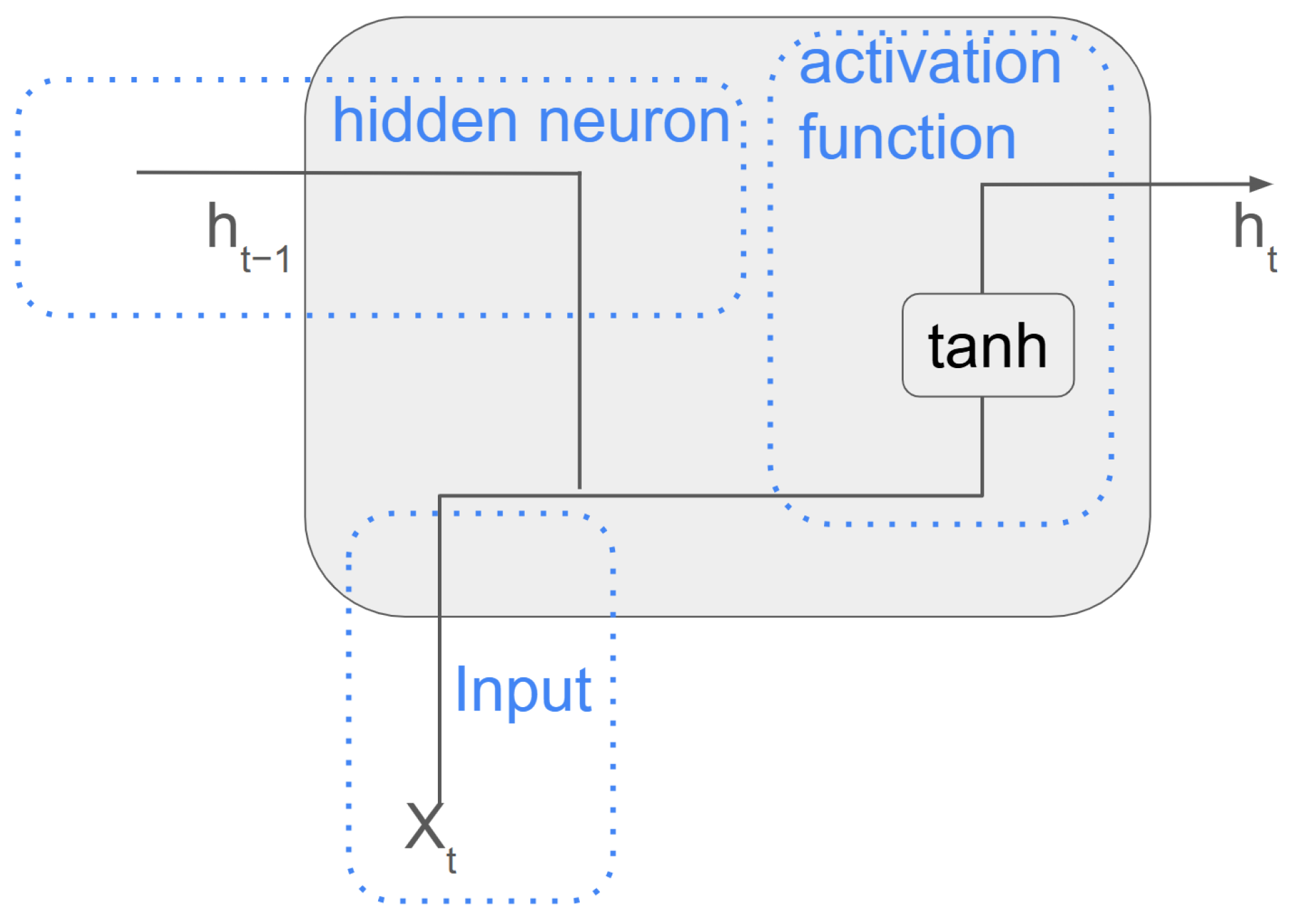
A particular class of these models, known as recurrent neural networks (RNNs), is especially suited for sequential data, such as time series or characteristic curves that vary with boundary conditions like voltage, temperature, and irradiance. RNNs differ from traditional ANNs by incorporating feedback loops, allowing the network to retain information from previous steps. These networks are used in difficult tasks such as recognition, machine translation, image captioning, and modeling I-V curves under varying environmental conditions [31]. In RNNs, the information flow is a little different from that of ANNs, as can be seen in Figure 3. In this case, the weights are characterized by $h_{t-1}$ and $X_t$. The $h_{t-1}$ is a weight which will be multiplied by the output from the previous neuron. With this, each RNN neuron is connected to the next one [30,32]. As with ANNs, there is an activation function to add non-linearity, as can be seen in Figure 3. In training, the weights are adjusted using an algorithm called Backpropagation Through Time (BPTT), which is responsible for calculating the output error and adjusting the weights, taking into account all previous steps in the sequence.

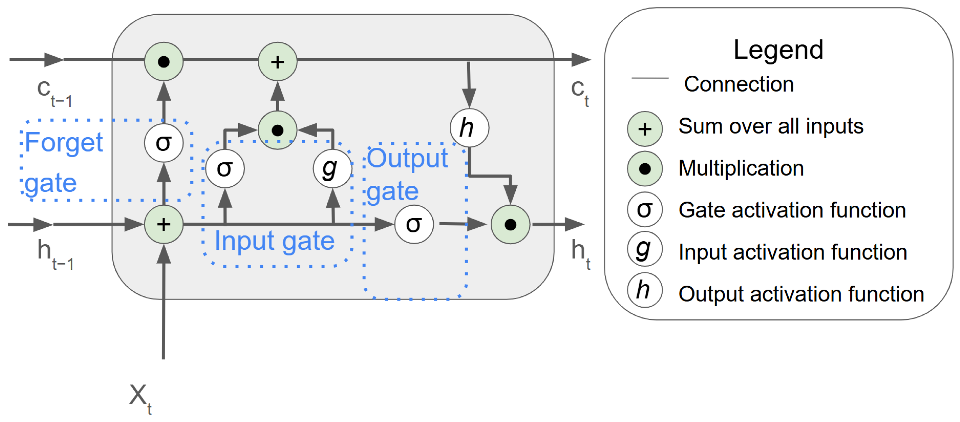
There is a problem in simple RNNs known as the vanishing gradient problem. This problem is a challenge for RNNs when they try to learn from very long sequences of data. During training, RNNs try to adjust the error using BPTT. However, when the data sequence is very large, the adjustment needed to be made to the sequence at the earliest step ends up becoming smaller and smaller. These weights end up decreasing so much that they practically disappear. As a result, the network can no longer learn or remember information that occurred early in the sequence, which impairs its ability to capture long-term relationships [32,33,34]. The long short-term memory (LSTM) is an alternative type of RNN that is more popular due to its architecture. This method solves a problem that exists in simple RNN [32,33,34]. The LSTM has a structure that can be classified as ‘gates’; these gates are responsible for having the memory of this neuron [34]. The neurons of an LSTM have a layout as three types of self-connected gates; these gates are responsible for allowing the reading, writing, and removal of information in memory [32]. The architecture of the LSTM is illustrated in Figure 4, which illustrates the complex calculations existing in a cell LSTM with the three gates represented. One way to understand these three gates is that they work as filters. The forget gate is responsible for deciding which data should be erased from memory (this behavior is developed by the use of the activation function and mathematical calculation), the input gate decides what should be stored in memory, and the output gate decides what from memory should be used. Like the simple RNN, this cell inputs previous data, but in this case, the LSTM has two states, one called the cell state (the weight value is $C_{t-1}$ in Figure 4) and a hidden state (the weight values is $h_{t-1}$ in Figure 4) and the current data period (with weight denominated $X_t$). The LSTMs have hidden weights associated with the gates, so there are multiple weights to adjust in each LSTM cell. The LSTMs also use BPTT to adjust weights during training.

LSTM is very accurate, but it has a high computational cost. There are several weights to be adjusted, and one way to improve LSTM was the development of the Gated Recurrent Unit (GRU), which can be considered a variant of the LSTM proposed by Chung in 2014 [35]. The difference between LSTM and GRU is how their gates monitor information flow; the GRU has two gates called reset and update [35,36,37]. The update gate decides how much of the memory should be maintained and how much of the new information should be used; it is like saying “this is still important, let us keep remembering it”. The second gate is the reset gate; it decides how much of the old memory should be kept and how much new information should be used—it is like saying “that does not matter anymore, let us start from scratch here” [36]. Figure 5 is illustrated the GRU, and it is possible to see that GRUs have another difference between LSTM and GRU—the GRU has only cell state represented by $h_{t-1}$ and data of current period ($X_t$) with Tanh playing the role of activation function [36].

There are numerous options for activation functions, such as Sigmoid, Tanh, ReLU, Linear, and others. In general, these functions were responsible for introducing nonlinearity in the neural network. These functions work with input values by transforming them, for example, ReLU transforms them to zero if the input value is negative, the sigmoid transforms the input value to the range zero to one, the Tanh transforms the input value to the range negative one to one, and other transformations take place.

In this work, LSTM and GRU architectures with a bidirectional method were employed to predict the output current of a polycrystalline silicon solar cell based on input voltage, temperature, and irradiance, ultimately modeling the full I-V characteristic. These architectures were selected due to their proven robustness in handling nonlinear experimental data and multi-variable dependencies.

2. Materials and Methods

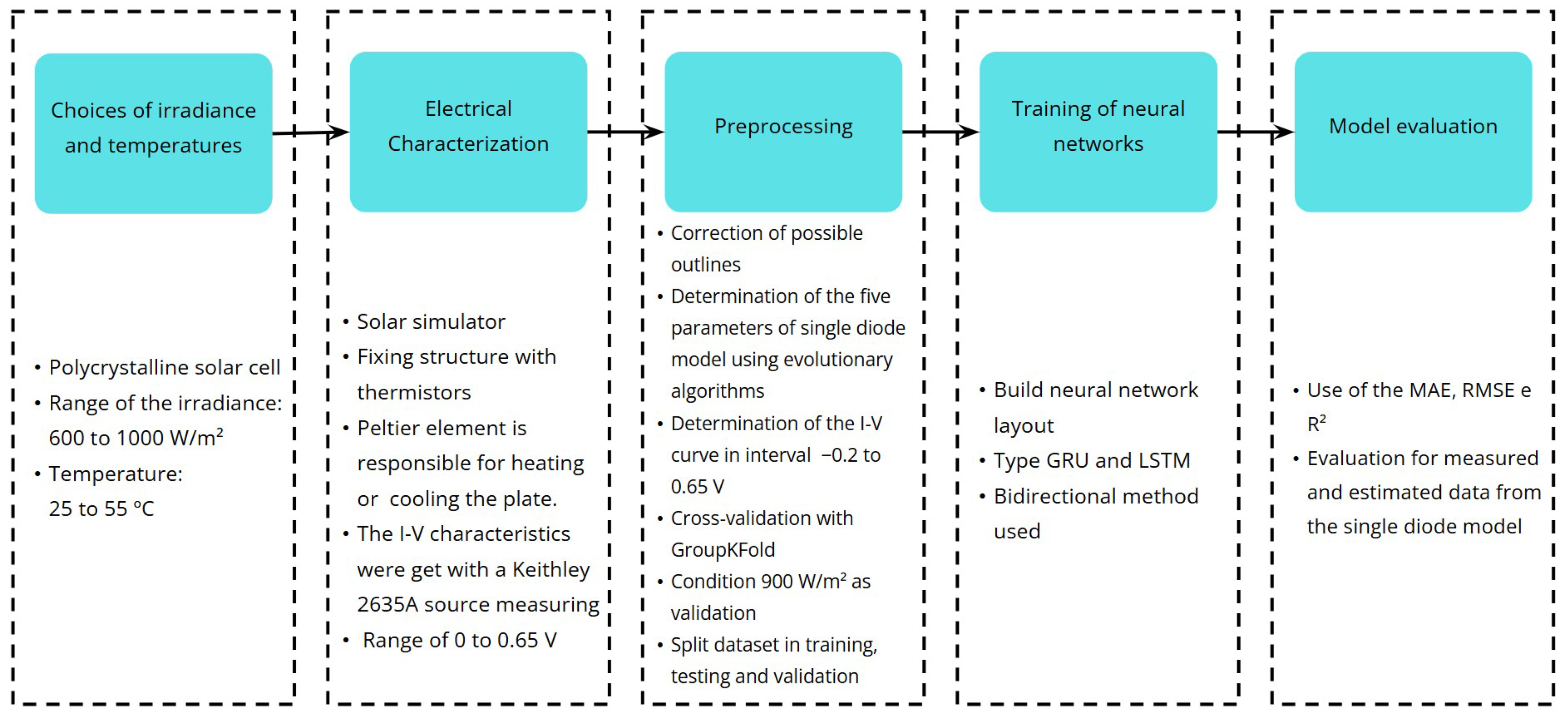
This section describes the materials, equipment, software, and methods used to achieve the objectives of this study. Figure 6 presents a flowchart summarizing the main experimental and analytical steps, detailed below.

2.1. Obtaining Datasets

The datasets were considered for different scenarios of the temperatures (°C) and irradiance (${\mathrm{W/m}}^2$). These scenarios chosen were temperature: 25 to 55 °C with a step of 5 °C and irradiance of 600 to $1000 {\mathrm{W/m}}^2$ with a step of $100 {\mathrm{W/m}}^2$ (the data are available in the Appendix A). One commercial polycrystalline silicon solar cell was used for this work.

The choice of irradiance values between 600 and $1000 {\mathrm{W/m}}^2$ was intended to simulate environments with partially cloudy skies, mornings, or late afternoons, which are the typical environmental conditions to which photovoltaic panels are exposed. The choice of temperature range was made so that data could be obtained to teach the models how the I-V curve would behave with temperature variation without irradiance variation. This strategy aims to provide data in different scenarios to the model, thus improving performance.

2.2. Experimental Procedure

The measurements of the I-V characteristics of the chosen polycrystalline solar cell (the parameter values provided by the manufacturer can be found in

Table 2. Parameter of the polycrystalline solar cell.

Parameter	Value
Power (W)	$0.045$
Maximum Power Point Current (A)	$0.087$
Maximum Power Point Voltage (V)	$0.52$
Short-circuit current (A)	$0.104$
Voltage Open Circuit (V)	$0.62$
Efficiency (%)	$17.57\%$
Dimension (mm)	50 × 19

) considered the temperature and irradiance conditions mentioned in Section 2.1. For each pair of illumination and temperature conditions, the measurements were repeated ten times in order to reduce the occurrence of measurement errors.

To generate stable and precise irradiance during the I-V acquisition, a solar simulator of the company Zundar, (located in Shanghai, China), model ZTHSO61L, was used (Figure 7a). This simulator has a 2500 W xenon lamp controlled by a power source that allows varying the radiation by controlling the output power. The determination of the correct irradiance level was determined by using a calibrated pyranometer Kipp & Zonen CM4 (The company is location in Sterling, VA, USA) with a resolution of 7 µV/Wm² and represented in Figure 7b.

The solar cell was positioned inside the solar simulator using a setup that fixed the solar cell tightly using an aluminum plate with a series of small holes and connected to a vacuum pump (Figure 7c). This plate houses two negative temperature coefficient (NTC) thermistors (an accuracy of 0.3 °C) (from company Ketotek localized in Xiamen, China), one inside and another on the upper surface very close to the solar cell. The aluminum plate is placed on top of a Peltier element TEC1-12715 from company Javino localized in Hong Kong, China, which is responsible for heating or cooling the plate. The electrical contacts were carried with two tungsten contact probes pressed over the painted cell interdigitated electrodes.

Finally, the I-V characteristics were measured with a Keithley 2635A from company Tektronix localized in Beaverton, OR, USA (Figure 7d) Source Measuring Unit (SMU) considering a range of 0 to 0.65 V with a step of 0.01 V. The accuracy of the SMU is ±(0.03% + 1.5 mA) up to 1 A, and the voltage has accuracy ±(0.02% + $350 \mathsf{\mu }$V) up to 2 V.

2.3. Error Metrics

The performance of the models was evaluated using mean absolute error (MAE), root mean square error (RMSE), and the coefficient of determination (R²). These error measurement equations are widely used to evaluate regressions.

MAE calculates the average of the absolute differences between the measured and estimated values, represented by Equation (4). In the equation, the N is the number of samples, $y_i$ is the observed value for each sample, and $\widehat{y_i}$ is the value predicted by the model for each sample

$$\mathrm{MAE}={\displaystyle \frac{1}{N}}\sum _{i=1}^N|y_i-\widehat{y_i}|$$

(4)

RMSE is similar to MAE, but it penalizes larger errors more significantly. Therefore, a high RMSE value indicates that there are points in the real data that the regression was unable to predict, as it squares the difference before taking the average, represented by Equation (5), where N is number of samples, $y_i$ is observed value for each sample, and $\widehat{y_i}$ is the value predicted by the model for each sample

$$\mathrm{RMSE}=\sqrt{{\displaystyle \frac{1}{N}}\sum _{i=1}^N{(y_i-\widehat{y_i})}^2}$$

(5)

R² is a metric that indicates how well your model fits the data. A value of 1.0 (100%) indicates a perfect fit, making it more suitable for comparing models, represented by Equation (6). The variables, N is the number of samples, $y_i$ is the observed value for each sample, $\widehat{y_i}$ is the value predicted by the model for each sample, and $\overline{y}$ is the average of the measured sample values.

$${\mathrm{R}}^2=1-{\displaystyle \frac{{\sum }_{i=1}^N{(y_i-\widehat{y_i})}^2}{{\sum }_{i=1}^N{(y_i-\overline{y})}^2}}$$

(6)

2.4. Data Preprocessing

After collecting the experimental data, a preprocessing step was carried out to ensure data quality and consistency. Since each I-V curve was measured ten times under identical temperature and irradiance conditions, potential outliers were identified and corrected. A statistical approach based on the interquartile range (IQR) was used, replacing outlier values with the mean of the valid measurements for each condition.

To improve the neural network’s performance, it was chosen to derive the I-V curves from the measured data using evolutionary algorithms to solve Equation (3). This allowed us to obtain the negative voltage values observed in the first quadrant of the curve, since negative voltage values generate a very small reverse saturation current compared to the forward current. Therefore, the equipment required to measure reverse current could not be the same as that required to measure forward current, which must be capable of measuring at much higher currents. This is different from the currents observed in signal diodes. Measuring with different devices poses enormous challenges due to small systematic errors due as the calibration of high-current instruments interferes with the accuracy of the two quadrants for +V and −V.

Therefore, solving Equation (3) was the way to access the negative voltage data. Thus, the I-V curve was determined for each temperature and irradiance condition in the range from −0.2 to 0.64 V. With the I-V curve determined by Equation (3), these data were used to train the neural networks.

To evaluate the predictive performance of the neural network models, a cross-validation strategy was employed, with special consideration given to the structure of the dataset. A GroupKFold—a method present in Scikit-Learn version 1.5.1—validation approach was adopted because each set of measurements corresponds to a distinct environmental condition. This ensures that all data from a given condition are used exclusively for training or testing in each fold, preventing data leakage between training and test sets.

Additionally, one specific irradiance (900 W/m²) was reserved as an external validation set. This dataset was not used during model training and served to assess the models’ ability to generalize to unseen experimental conditions.

The dataset was split into training and testing using GroupShuffleSplit (this technique—a method present in Scikit-Learn version: 1.5.1—split the dataset randomly between training and testing, but respecting the groups) with a ratio of 10% for testing. With this, the datasets had a total of 15,000, 1800, and 4200 rows, respectively, for training, testing, and validation.

The neural networks were implemented in the Python language (version: 3.12.7) with the Pandas (version: 2.2.2) and Numpy (version: 1.26.4) libraries to analyze and manipulate the data, Scikit-Learn (version: 1.5.1) for data preprocessing, and TensorFlow (version: 2.16.2) to build the neural networks.

2.5. Modeling GRU and LSTM

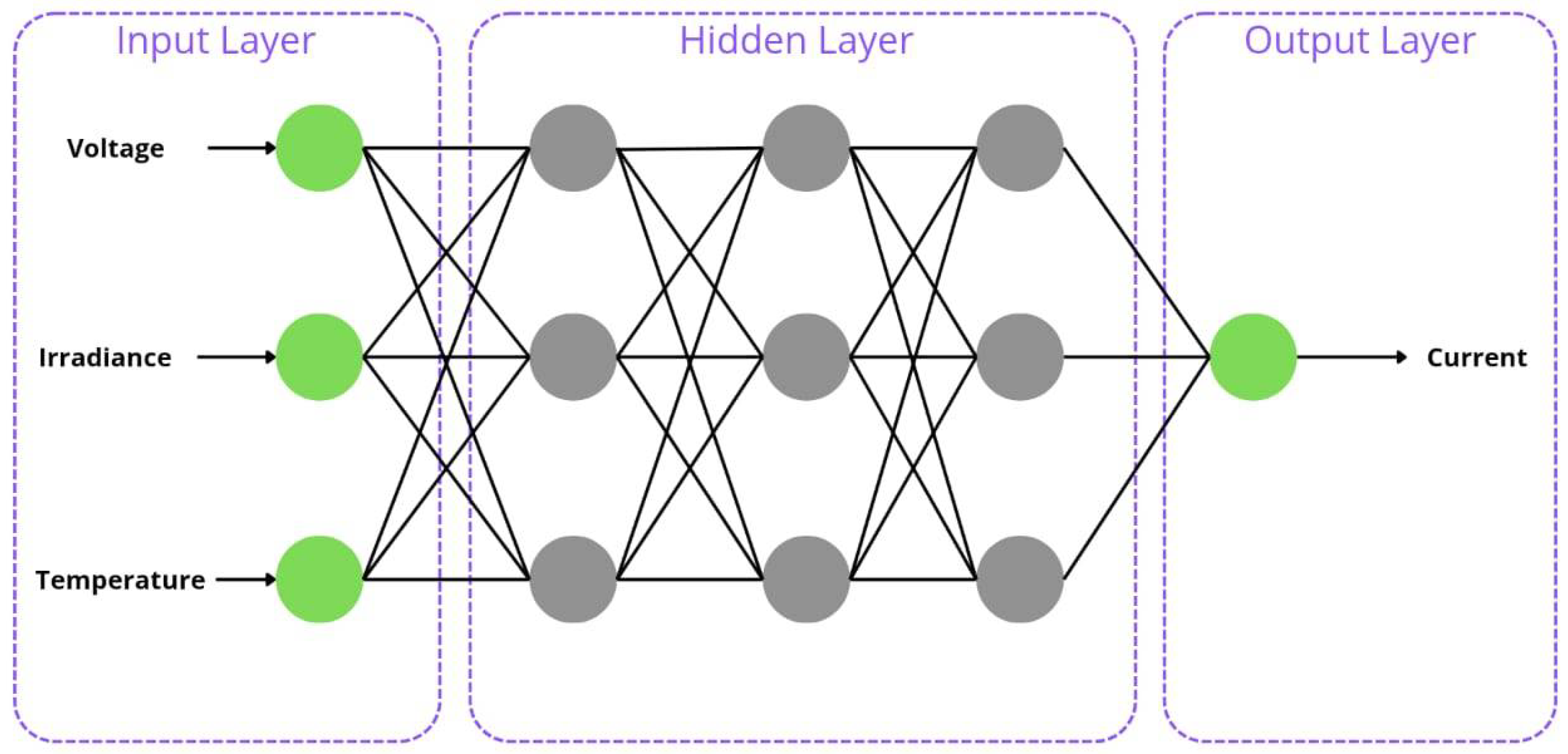
The neural network architecture is represented in Figure 8; it is of the fully connected type (all neurons are interconnected) and the input values are the electrical voltage, irradiance, and temperature. Since the objective is to find the current value, this architecture does regression work for the I-V characteristic curve. In the hidden layer, there are differences between the types of artificial neural networks, and their representation is shown in Table 3. Another method employed was the use of bidirectional in the LSTM and GRU layout (this method is characterized by the processing of data in both directions, that is, for each neuron of the RNN, there is an equal one, but which processes the data in the opposite direction. Both results of the neurons are combined to generate a more accurate output). Each model is represented in Table 3; the model based on GRU and LSTM has four layers in the hidden layer. The number of neurons in each layer is represented in Table 3, as well as the type of neuron. “Dropout” is a layer responsible for redefining part of the weight so that there are not overfitting problems (the rate value represented by the percentage of the previous layer would be reset randomly).

Each model used the same configuration for training, with the loss function being a mean squared error (MSE) and the optimizer being Adam (the Adam optimizer is used to adjust weights to the neural network during training; it combines the best property between adaptive gradient descent and momentum and it was proposed by Kingma and Be [38]). The library TensorFlow was used to build the neural networks. The batch size used was 10, meaning that the weights of the neurons will be updated every 10 samples.

Another point is the total number of parameters (weights) in each model; the GRU model has 6973, and the LSTM is 8635.

The choice to use the Swish function was made due to its characteristics. The Swish function is smooth and continuous throughout its domain, which helps to keep the gradients during training. Compared to the ReLU function (which has a discontinuity at zero), the Swish function allows negative values to pass smoothly, which can be useful to preserve information. In general, the Swish function tends to present better results when compared to ReLU. However, it has a higher computational cost, but since in this study the network does not have a very large number of parameters, it was possible to use it during the cross-validation test, and it was possible to observe an improvement in the results when compared to ReLU. Therefore, the Swish function was chosen instead of ReLU for training.

Table 3. Neural network architecture. GRU(Bidirectional) and GRU_1(Bidirectional) represent the use of GRU cells in a given neural network layer with with the bidirectional method; ANN and ANN_1 represented the use of ANN cells in a given neural network layer; LSTM(Bidirectional) and LSTM_1(Bidirectional) represent the use of LSTM cells in a given neural network layer with the bidirectional method.

GRU Model Architecture	LSTM Model Architecture	Number of the Neurons	Activation Function
Input	Input	-	-
GRU(Bidirectional)	LSTM(Bidirectional)	24	Tanh
ANN	ANN	24	Swish [39]
Dropout	Dropout	Rate: 0.1	-
GRU_1(Bidirectional)	LSTM_1(Bidirectional)	9	Tanh
ANN_1	ANN_1	1	Linear

Table 3. Neural network architecture. GRU(Bidirectional) and GRU_1(Bidirectional) represent the use of GRU cells in a given neural network layer with with the bidirectional method; ANN and ANN_1 represented the use of ANN cells in a given neural network layer; LSTM(Bidirectional) and LSTM_1(Bidirectional) represent the use of LSTM cells in a given neural network layer with the bidirectional method.

GRU Model Architecture	LSTM Model Architecture	Number of the Neurons	Activation Function
Input	Input	-	-
GRU(Bidirectional)	LSTM(Bidirectional)	24	Tanh
ANN	ANN	24	Swish [39]
Dropout	Dropout	Rate: 0.1	-
GRU_1(Bidirectional)	LSTM_1(Bidirectional)	9	Tanh
ANN_1	ANN_1	1	Linear

3. Results

With the architecture assembled and the data corrected, it was possible to train the neural networks. Before training, the GRU and LSTM models with the bidirectional method were evaluated using cross-validation with the GroupKFold method. This method is used when data are grouped by some common feature, for example, multiple measurements for the same feature (which is the case in this study). Thus, GroupKFold divides the dataset into subsets (folds), where in each iteration, one fold is used for training and one is reserved for testing. The process is repeated for all folds, ensuring that each fold is used exactly once as a test set.

This study was used in five folds, because the choice of five folds in GroupKFold is a strategic decision that balances validation quality, computational efficiency, and respect for the data structure. With a training set containing 16,800 samples, this division allows each fold to contain, on average, about 3360 samples, which is enough to ensure statistical diversity in each division.

During cross-validation, the models’ predicted data were compared with real data using the MAE, RMSE, and R² metrics. The average results obtained with GroupKFold are presented in

Table 4. The average error metrics for the models in cross-validation.

Model	MAE $\times {10}^{-3}$	RMSE $\times {10}^{-3}$	R2
GRU	$1.629$	$3.072$	$0.9926$
LSTM	$1.564$	$3.060$	$0.9923$

.

Analysis of the error metrics revealed that both approaches were able to describe the real data, as the MAE and RMSE values were low. In addition, the R² was very close to one, indicating that almost all the variability in the data was handled by the models. These metrics can thus be used for model training.

Another point is the computational cost; the GRU model had a training time of 7 min and 22 s, and the LSTM model had a training time of 8 min and 15 s. The callback strategy was used for the optimizer at training time (two callbacks were used, and both functions are native to TensorFlow. ReduceLROnPlateau has the function of reducing the learning rate when the models are at local minima, and the EarlyStopping function has a function to stop training if the model does not have a better error metric).

The time to calculate the parameters by the evolutionary algorithm for all conditions analyzed (considering that they were measured ten times for each condition) was 97 min and 55 s.

Table 5. The mean error metrics for the models with data estimated from Equation (3), solved by the evolutionary algorithm. The GRU model was the best model, with fewer associated errors.

Model	MAE $\times {10}^{-3}$	RMSE $\times {10}^{-3}$	R2
GRU	$1.456$	$3.051$	$0.9936$
LSTM	$1.311$	$3.343$	$0.9923$

shows the averages of the error metrics of the validation set, and as shown in Figure 9, the models lead to a set of parameters with a reasonable prediction for a scenario of 900 W/m² in the range 25 to 55 °C. For Figure 9, as the measurements were made ten times for the I-V curve, the plotted curve is an average of these measurements for use as model validation, and two temperatures are also plotted, 25 and 45 °C; the other temperatures can be evaluated using

Table 6. The RMSE for the models. At temperatures of 45 and 50 °C, the models showed the worst performance.

Temperature	RMSE Between GRU Model and Evolutionary Algorithms $\times {10}^{-3}$	RMSE Between GRU Model and Measured Data $\times {10}^{-3}$	RMSE Between LSTM Model and Evolutionary Algorithms $\times {10}^{-3}$	RMSE Between LSTM Model and Measured Data $\times {10}^{-3}$
25	$0.879$	$0.936$	$1.083$	$1.586$
30	$2.009$	$3.326$	$1.406$	$2.652$
35	$2.059$	$2.565$	$1.994$	$2.938$
40	$1.869$	$2.611$	$1.954$	$2.258$
45	$4.395$	$5.814$	$5.197$	$6.878$
50	$9.081$	$11.849$	$9.251$	$11.930$
55	$3.021$	$3.585$	$2.005$	$2.240$

, which shows the RMSE of all temperatures.

Using the measurement data, the RMSE, MAE, and R² metrics were calculated. The values are represented in

Table 7. The average error metrics for the models with measured data. The GRU model was the best model, with fewer associated errors.

Model	MAE $\times {10}^{-3}$	RMSE $\times {10}^{-3}$	R2
GRU	$2.813$	$5.790$	$0.9844$
LSTM	$2.613$	$5.858$	$0.9840$

. The RMSE and MAE values were low, and R² was close to one.

The results for the GRU model can be observed in the graph of Figure 9. The curve obtained with the model is in green. The prediction is very close to the average experimental data (in blue) and to the I-V curve predicted by the evolutionary algorithm (in orange). Table 6 shows metrics for validation data; the values MAE, RMSE, and R² confirm that the model managed to get very close to the evolutionary algorithm. It can be observed that all models presented greater errors at temperatures of 45 and 50 °C. Consequently, the graph for the 45 °C temperature is presented in Figure 9b; it is possible to observe that the error is in the short-circuit region (negative current).

In the LSTM model, there was behavior very close to real data, and the data are estimated by an evolutionary algorithm. The LSTM model in comparison to the GRU model was similar. The values of the MAE, RMSE, and R² shown in Table 5 models are very close, for example, the average MAE in the validation data was $1.311\times {10}^{-3}$ and GRU was $1.456\times {10}^{-3}$ A, a small difference. R² was very close to one for both models (in Table 5). Comparing each temperature in Table 6, in some scenarios, the GRU model was better, and LSTM was better in others. In the forecast graph, at temperatures of 25 and 45 °C (Figure 9), these small differences become clearer.

The validation leads to low error metric values, indicating that the proposed architecture is capable of fitting and predicting experimental data. Table 5 and Table 7 show that the GRU model shows the best results with the validation data. Regarding measurements with fewer data points, the test data, and the metrics measured (

Table 8. Metrics of the models with test data with fewer data points.

Model	MAE $\times {10}^{-3}$	RMSE $\times {10}^{-3}$	R2
GRU	$7.594$	$16.077$	$0.9848$
LSTM	$8.465$	$17.344$	$0.9823$

), the best model was LSTM_GRU.

Another simulation that was carried out used only irradiance data equal to 600 and 1000 W/m² with a temperature between 25 and 55 °C. This was carried out to verify whether the architecture model will be able to describe experimental data, with a smaller amount of data for training. There is a total of 8400 data points, consisting of voltage, temperature, and irradiance. Remembering that ten measurements were taken for each temperature, these data were used for the new training. The first training was with 15,000 data points, so neural networks tend to perform better with large data sets. Thus, this procedure is a test on how reducing the data size influences the accuracy of the models. The other data (irradiance between 700, 800, and 900 W/m²) were used to test, and the error metrics (MAE, RMSE, and R²) are shown in Table 8.

The training time was longer in the second training; the GRU model took 7 min and 51 s, and the LSTM took 8 min and 50 s.

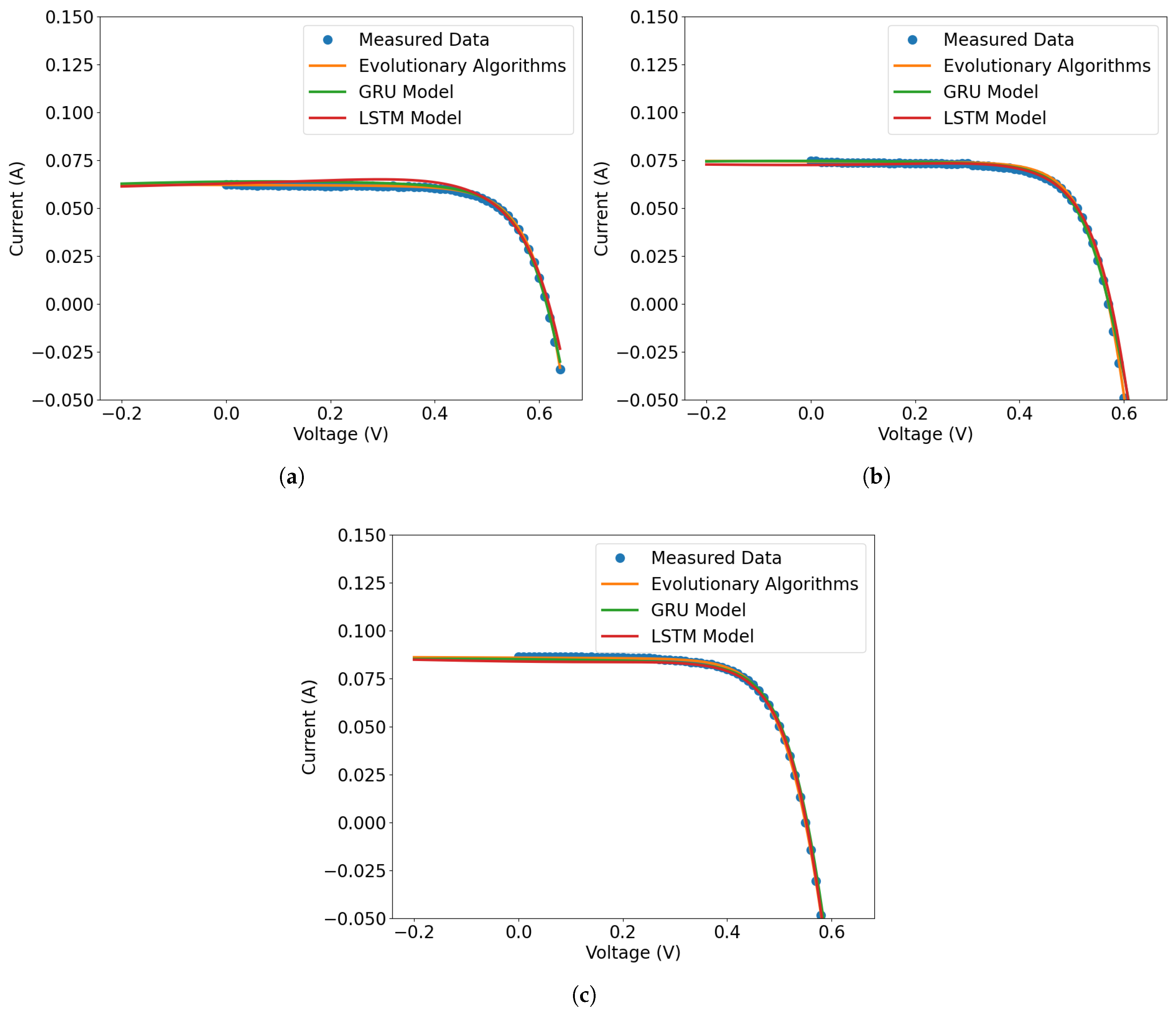
As expected, the model metrics got worse results, although R² values kept close to one. This is indicative of that model being able to describe the observed data. In Figure 10, some results for the test data are presented. The GRU model tends to improve its accuracy with an increase in temperature and irradiance.

The results demonstrate that both models—GRU and LSTM—were capable of accurately predicting the I-V characteristics of the solar cell under varying temperature and irradiance conditions. The GRU model exhibited the best overall performance, achieving the lowest error metrics while maintaining the shortest training time. Although the LSTM models produced similar results, their slightly higher computational cost and marginal improvements in accuracy suggest that GRU is the most efficient choice for this application. Additionally, when trained with a reduced dataset, all models experienced a small increase in error.

Comparing the results with the complete data and those with the reduced data, it can be seen that with the reduced data, the model had greater difficulty learning the behavior of the real data. This difficulty is associated with the complexity of the behavior of the I-V curve. Therefore, it is possible to conclude that the diversity and density of the input data—especially in relation to irradiance and temperature—are essential for the neural network to be able to accurately capture the variations in the current.

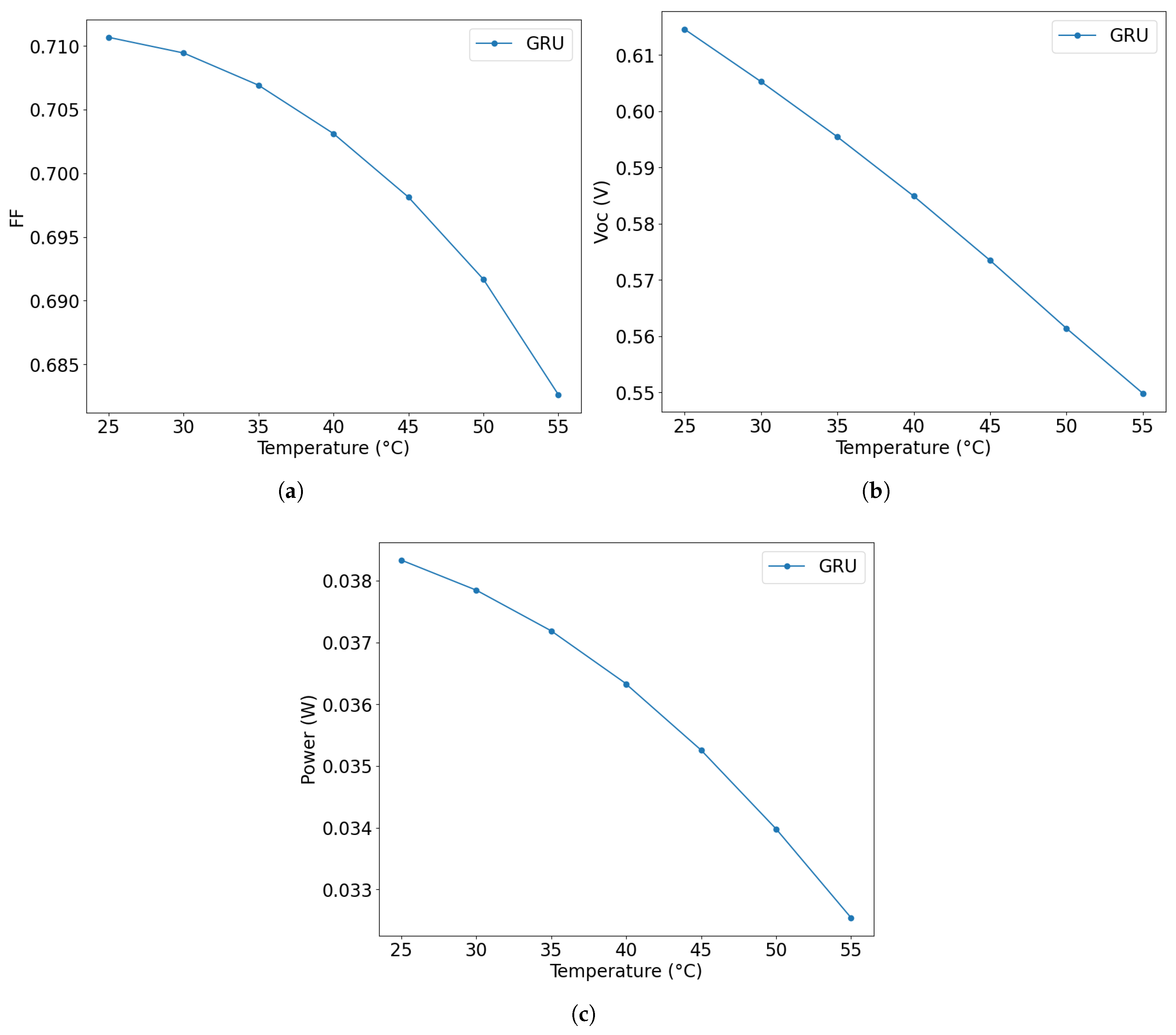
The physical consistency of the models’ I-V curves was assessed by extracting five key parameters from the single diode model (Equation (3)) for three scenarios: (a) a representative experimental measurement, (b) the reference condition at 900 W/m² and 25 °C, and (c) the model neural-predicted I-V curves under the same conditions. These parameters were obtained by fitting Equation (3) to both experimental and predicted curves using evolutionary algorithms. The extracted values are shown in

Table 9. Five main parameters obtained by traditional methods 900 W/m² and 25 °C.

Parameters	Data Types	Measured Data	GRU Model
$I_{ph}$	$0.09$ A	$0.087$ A	$0.087$ A
$I_0$	$1.01\times {10}^{-5}$ A	$6.18\times {10}^{-7}$ A	$4.40\times {10}^{-7}$ A
n	$1.64$	$2.03$	$1.949$
$R_s$	$0.04\mathrm{\Omega }$	$0.04\mathrm{\Omega }$	$0.09\mathrm{\Omega }$
$R_{sh}$	$1270\mathrm{\Omega }$	$919\mathrm{\Omega }$	$903\mathrm{\Omega }$

and compared across the three scenarios. Comparing the five parameters, the curve predicted by the GRU model had its results very close to the averaged data. Additionally, the parameters FF, $V_{OC}$, and $P_{MPP}$ were extracted from the I-V curve predicted by the GRU model, and the results are presented in Figure 11. A decreasing trend in Figure 11a $FF$ can be observed as temperature increases. This behavior is fully consistent with the behavior of photovoltaic devices. $V_{OC}$ exhibits a linear behavior (Figure 11b), decreasing with increasing temperature, a well-established phenomenon in semiconductor physics and essential for solar cell performance. As expected, $P_{MPP}$ also demonstrates a clear decrease with increasing temperature.

The values obtained for the n and $R_S$ differ from those commonly reported in the literature for crystalline silicon solar cells, which typically present n in the range of 1.2–1.5 and $R_S$ between 0.1 and $0.5 \mathrm{\Omega }$ [40,41]. In the present study, the n values were slightly higher (up to 2.03), while $R_S$ was lower (0.04–$0.09 \mathrm{\Omega }$). This discrepancy can be attributed to factors such as the specific test conditions adopted (900 W/m² and 25 °C), the possible aging of the module used, and the particularities of the parameter extraction method, which combines measured data with a GRU-type recurrent neural network-based model. Furthermore, parameter extraction from I-V curves at irradiances below the standard condition (STC) can lead to adjustments in the n and $R_S$ to compensate for variations in the photoelectric behavior of the cell. Similar results, with n greater than 2 and $R_S$ less than $0.1 \mathrm{\Omega }$, were also reported in studies that apply optimization methodologies or neural networks [42,43,44], reinforcing the plausibility of the values obtained in this work.

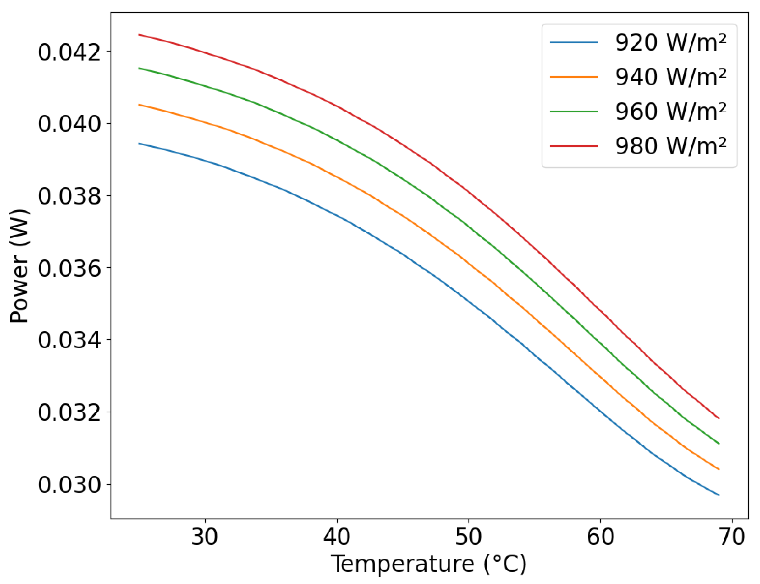
The GRU model (trained with complete data, as this presented the best results) was chosen to predict other scenarios and evaluate the behavior of solar energy cells. After predicting the I-V curve, the maximum power at a given temperature and irradiance was calculated using Equation (2); the results are shown in Figure 12. At each irradiance value, the temperature values were varied, and the I-V curve was estimated. From the I-V curve, the maximum power value was determined, and the values are plotted on the graph.

The model learned the behavior of the I-V curve, allowing the simulation of unmeasured scenarios and the estimation of the maximum power delivered by the solar cell in these scenarios. Another characteristic that can be evaluated is the behavior of the solar cell with temperature variation. In the GRU solar cell model, increasing the irradiance will only be beneficial if the temperature of the solar cell is controlled, since the behavior of the power is closely related to temperature and irradiance, where increasing the irradiance increases the power, but increasing the temperature reduces the power. This behavior is according with observed in the literature [45,46].

4. Discussion

This study investigated a new method for predicting the I-V curve for a polycrystalline silicon solar cell. The proposed strategy uses recurrent neural networks (LSTM and GRU) as the bidirectional method for estimating the current value, with inputs of irradiance, temperature, and voltage. In this sense, the models performed well, given that the error measurement results (RMSE and MAE) were considered low in the validation data.

Table 10. Comparison between different regression methods of the I-V characteristic curve.

Method	RMSE	R2
Random Forests-Based [47]	0.0091–0.2172	–
Regression Artificial Neural Network [48]	0.0130–0.0730	–
Mathematical model (Matlab/Simulink) [49]	0.1000–0.2600	0.9938–0.9625
Modified Taylor model [50]	0.0065–0.0156	–
Evolutionary algorithms [51]	0.0620–0.0720	0.9890–0.9992
Proposed method	0.0058–0.0173	0.9823–0.9848

shows a comparison of the most commonly used methods for regression of the I-V curve. Compared to other methods, the present study had the best metric in RMSE, where the value for the GRU-based model had the lowest associated error value.

4.1. Processing Time

A crucial point in using RNN is the processing time. Compared to the time to determine the I-V curves by solving Equation (3) using the evolutionary algorithm method, RNNs are more efficient. This study evaluated 350 I-V curves under different temperature and irradiance scenarios (five different irradiance and seven temperatures, with data collection performed ten times for each), with processing time exceeding 97 min. The time for training was 7 to 9 min (using the strategy to stop, the model does not improve accuracy), and after training, RNNs can predict these I-V curves in milliseconds.

There is another major advantage: considering the time required to obtain experimental data (characterization), trained models can estimate I-V curves simply by modifying the input variables, i.e., modifying the irradiance, temperature, and voltage values. Characterization requires more processing time and subsequent analysis.

4.2. Physical Properties

The efficiency and performance of solar cells are directly influenced by irradiance and temperature, as extensively documented in the literature [23]. Irradiance plays a crucial role, as it determines the amount of light energy converted into electricity. As illustrated in Figure 12, an increase in light intensity results in an increase in the cell’s output power.

In contrast, cell temperature has an inversely proportional effect on efficiency, being one of the main limiting factors. The negative impact of temperature is most visible in the $V_{OC}$ behavior, which decreases almost linearly with increasing temperature, as shown in Figure 11b. This voltage drop is attributed to the exponential increase in the reverse saturation current of the cell’s diode [52].

Therefore, a solar cell’s overall performance is the result of a complex balance between these two opposing effects. The ideal scenario for achieving maximum efficiency and power would be a combination of high irradiance and low temperature, such as that found on cold, sunny winter days, where the high current generated by light is not compromised by a heat-induced voltage drop.

5. Conclusions

The I-V characteristic curve of silicon solar cells provides access to various performance parameters, some of which are sensitive to temperature and illumination changes. While mathematical models may describe this curve well, the presence of transcendental variables makes their determination challenging. Neural networks offer an alternative approach to address this issue, which was the focus of this study.

To train these models, the I-V characteristic curves of polycrystalline silicon solar cells under different temperatures and lighting conditions were measured. Among the available neural network architectures, LSTM and GRU were selected. Model performance was evaluated using error metrics, with the GRU model achieving the best results: MAE = $2.813\times {10}^{-3}$, RMSE = $5.790\times {10}^{-3}$, and R² = $0.9844$. The other models had similar performance, with only minor variations in error metrics.

In terms of computational cost, the GRU model had the shortest training time with the full dataset, completing in 7 min and 22 s. When training with a reduced dataset, error metrics increased slightly, but the models still described the measured data well, as shown in Figure 10. In this case, the LSTM model had the lowest computational cost, with a training time of 8 min and 15 s. The use of recurrent neural networks with bidirectional for modeling the I-V characteristic curve proved to be a robust approach, leading to low error metrics. While differences in accuracy were observed between models, they were minimal. Training with a reduced dataset led to higher errors but maintained good fitting quality while reducing the computational cost. Overall, LSTM and GRU models are reliable approaches for modeling I-V curves. However, the GRU model demonstrated the best balance between accuracy and computational efficiency.

The GRU model was used to predict other scenarios, and the results were as expected for solar cells, another indication of the good performance of the model. With the predictions, it was possible to evaluate the performance of the solar cell, and the power of the solar cell is closely related to the temperature since the increase in the temperature of the surface of the solar cell reduces the power.

Evaluating the performance of the GRU and LSTM-based models, the accuracy was comparable to that of regression using the evolutionary algorithm of Equation (3). The I-V curves predicted by the artificial neural network models showed a notable overlap with those obtained by regression, as illustrated in Figure 9 and Figure 10. However, the gain in computational time is a notable point. Training the GRU/LSTM models was completed in approximately 8 min, while determining the parameters of Equation (3) and estimating the curves for the scenarios studied took approximately 97 min. This time difference represents a substantial improvement in process efficiency.

In neural network training, one of the biggest challenges is finding the balance between learning enough from the data and not learning too much. This balance directly influences the model’s ability to generalize to new data. A recurrent neural network model that has overfitted during training over-adjusts the network’s weights to the training data, capturing not only the real patterns but also the noise and outliers. This causes the model to perform excellently on the data it has already seen, but to fail when dealing with new data. During this study, dropout techniques (during training, some neurons are chosen to be turned off randomly) and early stopping (stopping training when an improvement does not occur) were used as a way to mitigate the risk of overfitting. The presented results demonstrate high robustness. However, since the database is limited, the risk of generalization still persists.

The study was developed using experimental data from polycrystalline solar cells, and for this type of material, the model’s accuracy can be considered good. However, as the I-V characteristic curves of other photovoltaic materials (thin-film and perovskite) were not present, the model’s behavior with these materials cannot be determined. It is believed that with a dataset with several types of solar cells, it would be possible to develop a model capable of predicting the current for the I-V curve from the temperature, irradiance, and voltage data. If generalizability is confirmed, application to photovoltaic equipment would be possible.

Based on the study’s findings and limitations, a natural next step is to expand the model’s capabilities to be more broadly applicable. A promising avenue for future research involves training the model on a more diverse dataset that includes thin-film and perovskite solar cells. This would allow for a comprehensive evaluation of the model’s performance across different photovoltaic technologies, moving beyond the current focus on polycrystalline cells.

References

1. Ivanova, V.; Rozhentsova, N.; Dautov, R. The analysis of the technical condition of power plants when using renewable energy sources in the territory of the Russian Federation. In Proceedings of the 2022 4th International Youth Conference on Radio Electronics, Electrical and Power Engineering (REEPE), Moscow, Russia, 17–19 March 2022; IEEE: Piscataway, NJ, USA, 2022; pp. 1–5. [Google Scholar] [CrossRef]
2. Zhang, X.; Ding, T.; Mu, C.; Han, O.; Huang, Y.; Shahidehpour, M. Dual Stochastic Dual Dynamic Programming for Multi-Stage Economic Dispatch With Renewable Energy and Thermal Energy Storage. IEEE Trans. Power Syst. 2024, 39, 3725–3737. [Google Scholar] [CrossRef]
3. Kumar, R.; Saha, R.; Simic, V.; Dev, N.; Kumar, R.; Banga, H.K.; Bacanin, N.; Singh, S. Rooftop solar potential in micro, small, and medium size enterprises: An insight into renewable energy tapping by decision-making approach. Sol. Energy 2024, 276, 112692. [Google Scholar] [CrossRef]
4. Ahmed, M.M.R.; Mirsaeidi, S.; Koondhar, M.A.; Karami, N.; Tag-Eldin, E.M.; Ghamry, N.A.; El-Sehiemy, R.A.; Alaas, Z.M.; Mahariq, I.; Sharaf, A.M. Mitigating Uncertainty Problems of Renewable Energy Resources Through Efficient Integration of Hybrid Solar PV/Wind Systems Into Power Networks. IEEE Access 2024, 12, 30311–30328. [Google Scholar] [CrossRef]
5. Liu, X.; Su, H.; Huang, Z.; Lin, P.; Yin, T.; Sheng, X.; Chen, Y. Biomass-based phase change material gels demonstrating solar-thermal conversion and thermal energy storage for thermoelectric power generation and personal thermal management. Sol. Energy 2022, 239, 307–318. [Google Scholar] [CrossRef]
6. Mathivanan, V.; Ramabadran, R.; Nagappan, B.; Devarajan, Y. Assessment of photovoltaic powered flywheel energy storage system for power generation and conditioning. Sol. Energy 2023, 264, 112045. [Google Scholar] [CrossRef]
7. Shen, S.; Yuan, Y. The economics of renewable energy portfolio management in solar based microgrids: A comparative study of smart strategies in the market. Sol. Energy 2023, 262, 111864. [Google Scholar] [CrossRef]
8. Patil, M.; Sidramappa, A.; Shetty, S.K.; Hebbale, A.M. Experimental study of solar PV/T panel to increase the energy conversion efficiency by air cooling. Mater. Today Proc. 2023, 92, 309–313. [Google Scholar] [CrossRef]
9. Lin, P.; Cheng, S.; Yeh, W.; Chen, Z.; Wu, L. Parameters extraction of solar cell models using a modified simplified swarm optimization algorithm. Sol. Energy 2017, 144, 594–603. [Google Scholar] [CrossRef]
10. Hevisov, D.; Sporleder, K.; Turek, M. I-V-curve analysis using evolutionary algorithms: Hysteresis compensation in fast sun simulator measurements of HJT cells. Sol. Energy Mater. Sol. Cells 2022, 238, 111628. [Google Scholar] [CrossRef]
11. Corrêa, H.P.; Vieira, F.H.T. Explicit three-piece quadratic model for accurate analytic representation of S-shaped solar cell current–voltage characteristics. Sol. Energy 2023, 258, 143–147. [Google Scholar] [CrossRef]
12. Piliougine, M.; Elizondo, D.; Mora-López, L.; Sidrach-De-Cardona, M. Photovoltaic module simulation by neural networks using solar spectral distribution. Prog. Photovolt. Res. Appl. 2013, 21, 1222–1235. [Google Scholar] [CrossRef]
13. Green, M. Solar Cells: Operating Principles, Technology, and System Applications; Prentice-Hall: Englewood Cliffs, NJ, USA, 1982. [Google Scholar]
14. Messenger, R.A.; Abtahi, A. Photovoltaic Systems Engineering; CRC Press: Boca Raton, FL, USA, 2018. [Google Scholar] [CrossRef]
15. Campanelli, M.B.; Osterwald, C.R. Effective irradiance ratios to improve I-V curve measurements and diode modeling over a range of temperature and spectral and total irradiance. IEEE J. Photovolt. 2016, 6, 48–55. [Google Scholar] [CrossRef]
16. Romero, H.F.M.; Hernández-Callejo, L.; Ángel González Rebollo, M.; Cardeñoso-Payo, V.; Gómez, V.A.; Aragonés, J.I.M.; Moyo, R.T. Optimized estimator of the output power of PV cells using EL images and I-V curves. Sol. Energy 2023, 265, 112089. [Google Scholar] [CrossRef]
17. Duran, E.; Piliougine, M.; Sidrach-De-Cardona, M.; Galan, J.; Andujar, J.M. Different methods to obtain the I-V curve of PV modules: A review. In Proceedings of the Conference Record of the IEEE Photovoltaic Specialists Conference, San Diego, CA, USA, 11–16 May 2008. [Google Scholar] [CrossRef]
18. Fébba, D.; Bortoni, E.; Oliveira, A.; Rubinger, R. The effects of noises on metaheuristic algorithms applied to the PV parameter extraction problem. Sol. Energy 2020, 201, 420–436. [Google Scholar] [CrossRef]
19. Ismail, H.A.; Diab, A.A. An efficient, fast, and robust algorithm for single diode model parameters estimation of photovoltaic solar cells. IET Renew. Power Gener. 2024, 18, 863–874. [Google Scholar] [CrossRef]
20. Deotti, L.M.P.; da Silva, I.C. A survey on the parameter extraction problem of the photovoltaic single diode model from a current–voltage curve. Sol. Energy 2023, 263, 111930. [Google Scholar] [CrossRef]
21. Abdulrazzaq, A.K.; Bognár, G.; Plesz, B. Enhanced single-diode model parameter extraction method for photovoltaic cells and modules based on integrating genetic algorithm, particle swarm optimization, and comparative objective functions. J. Comput. Electron. 2025, 24, 44. [Google Scholar] [CrossRef]
22. Seapan, M.; Hishikawa, Y.; Yoshita, M.; Okajima, K. Temperature and irradiance dependences of the current and voltage at maximum power of crystalline silicon PV devices. Sol. Energy 2020, 204, 459–465. [Google Scholar] [CrossRef]
23. Marion, B. A method for modeling the current-voltage curve of a PV module for outdoor conditions. Prog. Photovoltaics: Res. Appl. 2002, 10, 205–214. [Google Scholar] [CrossRef]
24. Liu, Y.; Ding, K.; Zhang, J.; Lin, Y.; Yang, Z.; Chen, X.; Li, Y.; Chen, X. Intelligent fault diagnosis of photovoltaic array based on variable predictive models and I-V curves. Sol. Energy 2022, 237, 340–351. [Google Scholar] [CrossRef]
25. Mellit, A.; Saǧlam, S.; Kalogirou, S.A. Artificial neural network-based model for estimating the produced power ofaphotovoltaic module. Renew. Energy 2013, 60, 71–78. [Google Scholar] [CrossRef]
26. Zhou, Y.; Chen, Z.; Jing, J.; Ma, L.; Feng, C.; Hou, J.; Xu, L.; Sun, M. Study on the mechanism of mismatched changes in photopotential and photocurrent at different temperatures and their impact on the photoinduced cathodic protection performance of ZnO. J. Alloys Compd. 2025, 1010, 177319. [Google Scholar] [CrossRef]
27. Giebink, N.C.; Wiederrecht, G.P.; Wasielewski, M.R.; Forrest, S.R. Ideal diode equation for organic heterojunctions. I. Derivation and application. Phys. Rev. B—Condensed Matter Mater. Phys. 2010, 82, 155305. [Google Scholar] [CrossRef]
28. Barbato, M.; Meneghini, M.; Cester, A.; Mura, G.; Zanoni, E.; Meneghesso, G. Influence of shunt resistance on the performance of an illuminated string of solar cells: Theory, simulation, and experimental analysis. IEEE Trans. Device Mater. Reliab. 2014, 14, 942–950. [Google Scholar] [CrossRef]
29. Wang, J.; Chankong, V. Recurrent Neural Networks For Linear Programming: Analysis And Design Principles. Comput. Oper. Res. 1992, 19, 297–311. [Google Scholar] [CrossRef]
30. Sarker, I.H. Deep Learning: A Comprehensive Overview on Techniques, Taxonomy, Applications and Research Directions. SN Comput. Sci. 2021, 2, 420. [Google Scholar] [CrossRef]
31. Rajagukguk, R.A.; Ramadhan, R.A.; Lee, H.J. A review on deep learning models for forecasting time series data of solar irradiance and photovoltaic power. Energies 2020, 13, 6623. [Google Scholar] [CrossRef]
32. Srivastava, S.; Lessmann, S. A comparative study of LSTM neural networks in forecasting day-ahead global horizontal irradiance with satellite data. Sol. Energy 2018, 162, 232–247. [Google Scholar] [CrossRef]
33. Hochreiter, S.; Schmidhuber, J. Long Short-Term Memory. Neural Comput. 1997, 9, 1735–1780. [Google Scholar] [CrossRef]
34. Raman, R.; Kumar, V.; Pillai, B.G.; Rabadiya, D.; Divekar, R.; Vachharajani, H. Forecasting Bitcoin Value with Hybrid LSTM-GRU Neural Networks. In Proceedings of the 2nd IEEE International Conference on Data Science and Information System, ICDSIS 2024, Hassan, India, 17–18 May 2024; Institute of Electrical and Electronics Engineers Inc.: Piscataway, NJ, USA, 2024. [Google Scholar] [CrossRef]
35. Chung, J.; Gulcehre, C.; Cho, K.; Bengio, Y. Empirical Evaluation of Gated Recurrent Neural Networks on Sequence Modeling. arXiv 2014, arXiv:1412.3555. [Google Scholar] [CrossRef]
36. Song, H.; Liu, X.; Song, M. Comparative study of data-driven and model-driven approaches in prediction of nuclear power plants operating parameters. Appl. Energy 2023, 341, 121077. [Google Scholar] [CrossRef]
37. Han, S.; Meng, Z.; Zhang, X.; Yan, Y. Hybrid deep recurrent neural networks for noise reduction of mems-imu with static and dynamic conditions. Micromachines 2021, 12, 214. [Google Scholar] [CrossRef]
38. Kingma, D.P.; Ba, J. Adam: A Method for Stochastic Optimization. arXiv 2014, arXiv:1412.6980. [Google Scholar] [CrossRef]
39. Ramachandran, P.; Zoph, B.; Le, Q.V. Searching for Activation Functions. arXiv 2017, arXiv:1710.05941. [Google Scholar] [CrossRef]
40. Sharma, A.; Sharma, A.; Averbukh, M.; Jately, V.; Azzopardi, B. An effective method for parameter estimation of a solar cell. Electronics 2021, 10, 312. [Google Scholar] [CrossRef]
41. Ćalasan, M.; Vujošević, S.; Krunić, G. Towards enhanced photovoltaic Modeling: New single diode Model variants with nonlinear ideality factor dependence. Eng. Sci. Technol. Int. J. 2025, 65, 102037. [Google Scholar] [CrossRef]
42. Sabadus, A.; Paulescu, M. On the nature of the one-diode solar cell model parameters. Energies 2021, 14, 3974. [Google Scholar] [CrossRef]
43. Almansuri, M.A.K.; Yusupov, Z.; Rahebi, J.; Ghadami, R. Parameter Estimation of PV Solar Cells and Modules Using Deep Learning-Based White Shark Optimizer Algorithm. Symmetry 2025, 17, 533. [Google Scholar] [CrossRef]
44. Cárdenas-Bravo, C.; Barraza, R.; Sánchez-Squella, A.; Valdivia-Lefort, P.; Castillo-Burns, F. Estimation of single-diode photovoltaic model using the differential evolution algorithm with adaptive boundaries. Energies 2021, 14, 3925. [Google Scholar] [CrossRef]
45. Amelia, A.R.; Irwan, Y.M.; Leow, W.Z.; Irwanto, M.; Safwati, I.; Zhafarina, M. Investigation of the effect temperature on photovoltaic (PV) panel output performance. Int. J. Adv. Sci. Eng. Inf. Technol. 2016, 6, 682–688. [Google Scholar] [CrossRef]
46. Al–bashir, A.; Al-Dweri, M.; Al–ghandoor, A.; Hammad, B.; Al–kouz, W. Analysis of effects of solar irradiance, cell temperature and wind speed on photovoltaic systems performance. Int. J. Energy Econ. Policy 2020, 10, 353–359. [Google Scholar] [CrossRef]
47. Ibrahim, I.A.; Hossain, M.J.; Duck, B.C. An Optimized Offline Random Forests-Based Model for Ultra-Short-Term Prediction of PV Characteristics. IEEE Trans. Ind. Inform. 2020, 16, 202–214. [Google Scholar] [CrossRef]
48. Khatib, T.; Ghareeb, A.; Tamimi, M.; Jaber, M.; Jaradat, S. A new offline method for extracting I-V characteristic curve for photovoltaic modules using artificial neural networks. Sol. Energy 2018, 173, 462–469. [Google Scholar] [CrossRef]
49. Jenkal, S.; Kourchi, M.; Yousfi, D.; Benlarabi, A.; Elhafyani, M.L.; Ajaamoum, M.; Oubella, M. Development of a photovoltaic characteristics generator based on mathematical models for four PV panel technologies. Int. J. Electr. Comput. Eng. (IJECE) 2020, 10, 6101. [Google Scholar] [CrossRef]
50. Lun, S.-x.; Du, C.-j.; Guo, T.-t.; Wang, S.; Sang, J.-s.; Li, J.-p. A new explicit I-V model of a solar cell based on Taylor’s series expansion. Sol. Energy 2013, 94, 221–232. [Google Scholar] [CrossRef]
51. Muhsen, D.H.; Ghazali, A.B.; Khatib, T.; Abed, I.A. A comparative study of evolutionary algorithms and adapting control parameters for estimating the parameters of a single-diode photovoltaic module’s model. Renew. Energy 2016, 96, 377–389. [Google Scholar] [CrossRef]
52. Ghani, F.; Rosengarten, G.; Duke, M.; Carson, J.K. On the influence of temperature on crystalline silicon solar cell characterisation parameters. Sol. Energy 2015, 112, 437–445. [Google Scholar] [CrossRef]
Figure 1. P-V characteristic curves at constant illumination of 1000 W/m2 for a temperature range from 25 °C to 55 °C with step 10 °C.
Electronics 14 03342 g001
Figure 2. Illustration of a simple artificial neuron, also known as a perceptron. Data are input into the artificial neuron and the input values are multiplied by weights (these values are numbers belonging to real numbers). Then the results are added together and the activation function is applied (this function is responsible for adding nonlinearities to the neuron).
Electronics 14 03342 g002
Figure 3. Illustration of an RNN with data flow among neurons.
Electronics 14 03342 g003
Figure 4. Illustration of the architecture of an LSTM cell.
Electronics 14 03342 g004
Figure 5. The structure of a GRU cell.
Electronics 14 03342 g005
Figure 6. Flowchart of work steps.
Electronics 14 03342 g006
Figure 7. Equipment used to characterize photovoltaic cells. In (a) is a Zundar solar simulator, model ZTHSO61L, with a 2500 W xenon lamp. In (b) is a Kipp & Zonen CM4 pyranometer; this was used to measure solar irradiance and ensure characterization conditions were correct. In (c) is the solar cell holder, used to position the cell precisely during testing. In (d) is a Keithley multimeter, model 2635A, used to measure the I-V characteristics curve of the photovoltaic cell.
Electronics 14 03342 g007
Figure 8. Illustration of the neural network architecture. The architecture is divided into three parts: input, hidden layer, and output. At the input, the values of voltage, radiation, and temperature are provided to the network. In the hidden layer, there are several artificial neurons represented by the gray circles. Since the architecture of this network is of the fully connected type, all neurons are interconnected (represented by the black lines). At the end, the network estimates the value of the current.
Electronics 14 03342 g008
Figure 9. Forecasts for the models and data measured at 900 W/m2. The forecasted data are in orange and green, while the measured data are in blue. In (a) is the plot for the 900 W/m2 and 25 °C, where the predicted data is very close to the measured data, and there are small differences between the models. In (b) is the plot for the 900 W/m2, and the 45 °C scenario is shown.
Electronics 14 03342 g009
Figure 10. The forecasts made from the models for weaker datasets and measured data for 700, 800, and 900 W/m2 at temperatures of 25, 45, and 55 °C. The predicted data in orange and green are the predictions for GRU and LSTM, respectively. Measured data are in blue. In (a), the plot is presented for the predictions of the 700 W/m2 scenario at 25 °C. The GRU model presented predicted data very close to the measured data, and the behavior of the prediction curve is very close to the measured data. The graph for 800 W/m2 at 45 °C and 900 W/m2 at 55 °C scenarios are shown in (b,c), respectively. In these scenarios, the GRU model performed best, although all models produced forecast data very close to the measured data.
Electronics 14 03342 g010
Figure 11. Graph of solar cell performance properties for 900 W/m2 irradiance. In (a) is the variation in F F with temperature, as predicted by the GRU model. Note the decrease in F F with increasing temperature, in agreement with the expected physical behavior. In (b) is V O C behavior as a function of temperature, obtained by the GRU model. The reduction in Voc with increasing temperature is consistent with solar cell physics. In (c) is P M P P predicted by the GRU model as a function of temperature. The reduction in maximum power with increasing temperature is a physically expected result and reproduced by the model.
Electronics 14 03342 g011
Figure 12. Power forecast for other scenarios irradiance ( W/m 2 ) and of temperature range from 25 °C to 70 °C with step 1 °C.
Electronics 14 03342 g012