Article

Deep Residual Shrinkage Network Recognition Method for Transformer Partial Discharge

College of Electrical and Electronic Engineering, North China Electric Power University, Baoding 071003, China
*
Author to whom correspondence should be addressed.
Electronics 2025, 14(16), 3181; https://doi.org/10.3390/electronics14163181
Submission received: 20 July 2025 / Revised: 6 August 2025 / Accepted: 8 August 2025 / Published: 10 August 2025

Abstract

Partial discharge (PD) is not only a critical indicator but also a major accelerating factor of insulation degradation in power transformers. Accurate identification of PD types is essential for diagnosing insulation defects and locating faults in transformers. Traditional methods based on phase-resolved partial discharge (PRPD) patterns typically rely on expert interpretation and manual feature extraction, which are increasingly being supplanted by Convolutional Neural Networks (CNNs) due to their ability to automatically extract features and deliver high classification accuracy. However, the inherent subtlety and diversity of characteristic differences among PRPD patterns, coupled with substantial noise resulting from complex electromagnetic interference, present significant hurdles to achieving accurate identification. This paper proposes a transformer partial discharge identification method based on Deep Residual Shrinkage Network (DRSN) to address these challenges. The method integrates dual-path feature extraction to capture both local and global features, incorporates a channel-domain adaptive soft-thresholding mechanism to effectively suppress noise interference, and utilizes the Focal Loss function to enhance the model’s attention to hard-to-classify samples. To validate the proposed method, given the scarcity of diverse real-world transformer PD data, an experimental platform was utilized to generate and collect PD data by artificially simulating various discharge defect models, including tip discharge, surface discharge, air-gap discharge and floating discharge. Data diversity was then enhanced through sample augmentation and noise simulation, to minimize the gap between experimental data and real-world on-site data. Experimental results demonstrate that the proposed method achieves superior partial discharge recognition accuracy and strong noise robustness on the experimental dataset. For future work, it is essential to collect more real transformer PD data to further validate and strengthen the model’s generalization capability, thereby ensuring its robust performance and applicability in practical scenarios.

1. Introduction

Power transformers are vital to power system stability, and their operational status directly impacts system safety. Insulation defects are a major cause of transformer failures and can lead to severe consequences [1]. Under strong electric fields, these defects can readily trigger partial discharge (PD), which in turn accelerates insulation degradation and may ultimately cause catastrophic failure. As both a cause and indicator of insulation deterioration, PD plays a crucial role in transformer condition monitoring. Accurate identification of PD types is essential for diagnosing insulation defects and locating faults. However, the complex structures and diverse fault mechanisms within transformer insulation systems lead to subtle differences in the discharge signal characteristics of various defect types. Furthermore, on-site detection is often plagued by noise from electromagnetic interference, which can mask or distort true discharge signal characteristics, significantly complicating transformer PD identification [2,3,4,5].
Traditional partial discharge identification methods recognize PD types by analyzing parameters such as pulse amplitude, waveform, frequency spectrum or time-frequency energy distribution [6,7,8,9]. However, these approaches often fail to fully leverage the intrinsic phase relationship between the discharge signal and the power frequency phase, provide insufficient reflection of the underlying physical discharge mechanism, and are susceptible to misjudgments or missed detections due to noise interference.
Phase-Resolved Partial Discharge (PRPD) characterizes PD patterns using three-dimensional features of phase, amplitude, and frequency. Different insulation defects generate distinct fingerprint-like patterns in PRPD images, making PRPD an effective tool for PD pattern recognition. However, manual interpretation relies heavily on expert experience and is increasingly being replaced by AI-driven automated methods.
Traditional machine learning recognition methods manually design and extract statistical or shape features such as pulse amplitude, phase, frequency, skewness, steepness, correlation coefficient of PRPD image, and then input the features into KNN (k-nearest neighbors), neural network, Bayesian classifier, support vector machines (SVM), random forest or other classification algorithms for pattern recognition [10,11,12]. However, manual feature engineering heavily relies on the designer’s domain expertise, and the incompleteness or limitations of the handcrafted features often result in critical information loss or inadequate representation within the PRPD patterns. This hampers the accurate capture and effective differentiation of diverse discharge patterns under complex working conditions, thereby compromising the overall accuracy of partial discharge identification. Deep learning technology, especially convolutional neural networks (CNNs), has developed rapidly in recent years. By automatically extracting features from raw data and performing classification tasks in an end-to-end manner [13,14], deep learning offers a new paradigm for automated PRPD pattern analysis [15,16,17]. Reference [18] fused PRPD images obtained under different applied voltage frequencies into a CNN with three-channel inputs, thereby enabling automated feature extraction and pattern recognition of PRPD. References [19,20] employed the ResNet model for PRPD recognition, achieving significantly higher accuracy than traditional machine learning methods including neural networks and SVM. Reference [21] applied three CNN models—VGG, InceptionV3 and Resnet50—to the recognition of PRPD patterns, with all models achieving exceeding 92%. Although deep learning methods have made significant advancements in PRPD pattern recognition, the related research remains relatively limited, particularly in scenarios involving noise interference.
The Deep Residual Shrinkage Network (DRSN) [22], proposed by Zhao et al. in 2020, is a deep learning model designed specifically for noisy data. By integrating soft-thresholding techniques from signal processing with a residual learning framework, DRSN achieves adaptive noise suppression, offering an approach for feature learning in noisy environments. In this paper, the DRSN is applied into transformer partial discharge recognition. The DRSN network structure is tailored to the characteristics of PRPD pattern recognition, employing dual-path feature extraction to capture both local details and global structural features of PRPD, incorporating an adaptive soft threshold shrinkage mechanism to effectively suppress noise, and introducing Focal Loss function to enhance model’s focus on misclassified samples during training, thereby enabling end-to-end PRPD pattern recognition. To validate the proposed method, due to the scarcity of diverse real-world transformer PD data, an experimental platform was employed to simulate various defect modes, including tip discharge, surface discharge, air-gap discharge and floating discharge, for collecting PRPD data. To bridge the gap between experimental and real-world on-site conditions, data diversity was significantly augmented via sample augmentation and noise simulation, thereby constructing diverse types of datasets. Experimental analysis shows that the features extracted by the DRSN model exhibit significantly better inter-class separability compared to classic CNN models. The average partial discharge identification accuracy exceeds 98% on the non-noisy experimental dataset, and reaches 96% on the experimental dataset with added simulated noise, significantly outperforming traditional CNN models. Finally, the generalization performance of the method is analyzed through case studies. For subsequent research, the collection of more actual transformer PD data is imperative to thoroughly validate the proposed model and bolster its generalization capability. This will be instrumental in ensuring its robust performance and applicability within practical environments.

2. Deep Residual Shrinkage Network and Its Improvement

To mitigate the performance degradation of deep neural networks in noisy environments, DRSN incorporates a soft-thresholding shrinkage mechanism into its network framework. This enables the network to adaptively suppress noise interference while preserving its depth, thereby improving the model’s robustness in complex environments [19]. Furthermore, this paper introduces the Focal Loss function into DRSN to improve the model’s attention to misclassified samples and alleviate the impact of sample imbalance on classification.

2.1. Deep Residual Shrinkage Network Structure

The deep residual shrinkage network (DRSN) employs the classic residual connection method to build its basic framework, with the residual shrinkage block (RSB) as its core module. The overall network architecture is composed of multiple RSBs stacked together, and the structural workflow includes: input → convolution block → RSB × M → Global Average Pooling (GAP) → Fully Connected (FC) layer × N → Softmax classification output.
The RSB structure, shown in Figure 1, is composed of three parts:
(1)
Basic residual block
Through identity connections, the input x is propagated across the intermediate layers and added to the output F(x), which is obtained through the convolution and soft-thresholding shrinkage operations. The results in the final network output   H x   =   F x   +   x . The learning goal of the network has changed from the output H x   to the residual function F x , which alleviates the degradation problem caused by vanishing or exploding gradients with the increase in network layers, and enhances the stability of training.
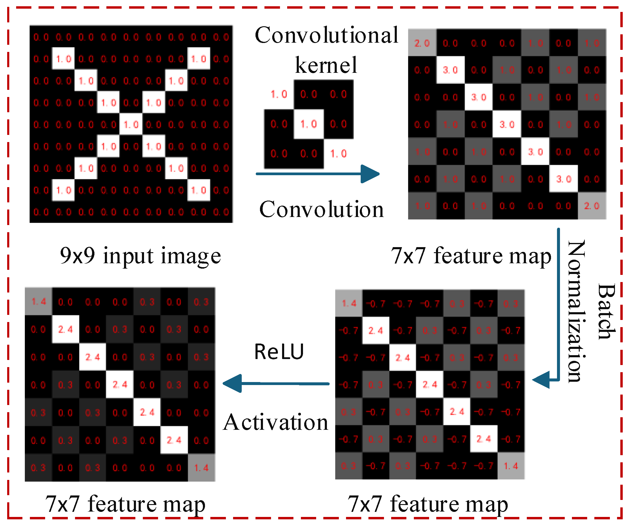
The basic residual block consists of two basic convolutional layers, each comprising a 3 × 3 convolution, batch normalization (BN) and the ReLU activation function. As illustrated in Figure 2, the convolution operation extracts local features by sliding the convolution kernel over the input data to generate feature map. Different convolution kernels can learn different features, such as contours, textures, etc. Batch normalization adjusts the feature map to a stable distribution with a mean of 0 and a standard deviation of 1 to accelerate training. The ReLU activation function introduces nonlinear operations, enabling the network to learn complex nonlinear mappings and thereby enhancing the model’s representational capacity.
An input image with dimensions H   ×   W   ×   C i n     (where H   ×   W is its spatial size and C i n is the number of channels) is processed through two convolutional layers followed by soft thresholding, resulting in an output of H 2   ×   W 2   ×   C 2 . In residual connections, if C i n C 2 , the input dimension is adjusted to C 2 via a 1 × 1 convolution to ensure consistency with the dimension of the soft thresholding output.
(2)
Adaptive soft-thresholding generative network
The mechanism operates by modeling inter-channel dependencies, dynamically adjusting the importance of channel features, and then adaptively generating soft thresholds for feature maps. The specific operations include:
a. Squeeze: Take the absolute value of the network’s input feature map to ensure that the elements are non-negative. Then, Global average pooling (GAP) is performed on the absolute-valued feature map for each channel, compressing the map of size   H 2   ×   W 2   ×   C 2   into the channel statistic of 1   ×   1   ×   C 2   according to Equation (1). This process effectively condenses the global spatial information into a channel descriptor, where Z c is the compressed value of the c - t h channel.
Z c = 1 H 2 ×   W 2 i = 1 H 2 j = 1 W 2 a b s   ( x c   ( i , j ) )
b. Excitation: Through the bottleneck structure of two FC layers, the nonlinear relationships between channels are learned, enabling the generation of channel weights. The first FC layer, using ReLU activation, reduces the dimension to C/r, where r is the compression ratio. The second FC layer restores the original number of channels and applies the Sigmoid activation function to adjust the output to a weight between 0 and 1. The calculation process for the excitation stage is shown in Equation (2), where δ represents the ReLU function, σ is the Sigmoid function, and W 1   and W 2 are the parameters of the two FC layers.
S c = σ   ( W 2   δ   W 1     Z c
c. Soft threshold generation: Multiply the learned channel attention weight S c with the channel mean Z c obtained from GlobalAvgPool to generate the feature map’s soft threshold τ c . Here, τ c represents the soft threshold of c - t h channel.
τ c = S c × Z c
d. Soft-thresholding layer: The nonlinear transformation is performed as described in Equation (4). The output feature map Y from the residual block’s convolution layer is shrunk channel by channel according to the soft threshold τ to suppress the noise characteristics. This layer is the core step of the denoising process.
F Y = Y τ × sign ( Y )         i f Y > τ 0                                                     others
Here, τ is soft threshold parameters ( τ > 0), sign (Y) is symbolic function. The relationship between the input and output of soft thresholding is shown in Figure 3.

2.2. Loss Function

To enhance the model’s attention to misclassified samples and mitigate the effects of data imbalance in the PRPD dataset on its recognition performance, the Focal Loss function is introduced into the network. The function formula is as follows:
F L   p , y   =   i   =   1 C a i   ( 1     p i ) γ y i l o g   ( p i )
Here, p   = ( p 1 , p 2 , , p C ) represents the predicted probability distribution of the sample. p i is the predicted probability that the sample belongs to the i -th discharge class. C is the number of classes.   y   = ( y 1 , y 2 , , y C ) is the true label, represented by a one-hot vector.
γ is the focusing parameter ( γ   0 ), which is used to control the penalty intensity for difficult and easy samples. When the value is 0, it degenerates to the standard cross entropy; the larger the value, the more attention is paid to difficult samples.
α i is the class balance factor, calculated as show in Equation (6), where N t o t a l represents the total number of samples and N i is the number of samples in the i -th class.
α i = N t o t a l C × N i + ε
The Focal Loss function dynamically calculates the class balance factor α i based on the number of samples in each class to alleviate the class imbalance problem.

3. Partial Discharge Recognition Based on DRSN

3.1. The Network Structure of DRSN Model

Deep networks construct composite functions f x   = f n f n 1   ( f 1 x ) by stacking nonlinear transformations layer by layer, with each layer learning features at different levels of abstraction. Network depth (i.e., number of layers) is a key dimension in the design of deep learning models. When the network is shallow, its ability to extract complex semantics is limited and its representational power is insufficient; when the network becomes too deep, it may lead to issues such as excessive computational resource consumption and overfitting.
Based on the conventional ResNet18 architecture, its original residual modules are replaced with RSBs, and the network structure is adjusted to align with the input and output dimensions required for PRPD pattern recognition. The network structure for PRPD pattern recognition is constructed as shown in Figure 4, with detailed parameters listed in Table 1. The model contains 18 weighted operation layers. The initial convolution layer (Conv2d+BN+ReLU) employs a 7 × 7 receptive field to extract the foundational features from input PRPD images. Normalization and activation operations serve to stabilize training process and enhance nonlinear representation. The Max Pooling layer (MaxPool2d) then reduces the spatial dimensions of the feature map, thereby highlighting key information and decreasing subsequent computational overhead. The backbone network is organized into four residual shrinkage stages, each containing two modules in series, either standard or downsampling RSB. The soft threshold shrinkage mechanism is applied within these blocks to suppress noisy features, and the identity connection is used to residual learning to mitigate vanishing gradients in deep networks. By adjusting the stride and channel count, the feature map is spatially downsampled and channel-expanded, enabling the progressive extraction of higher-level features. At the classification layer, the Global Average Pooling (GlobalAvgPool) aggregates spatial information into channel-level features, thereby reducing parameters and mitigating overfitting. Finally, the FC layer maps these features to the class space and applies a Softmax activation function to generate class probabilities for the partial discharge recognition task.

3.2. Partial Discharge Identification Algorithm Flow

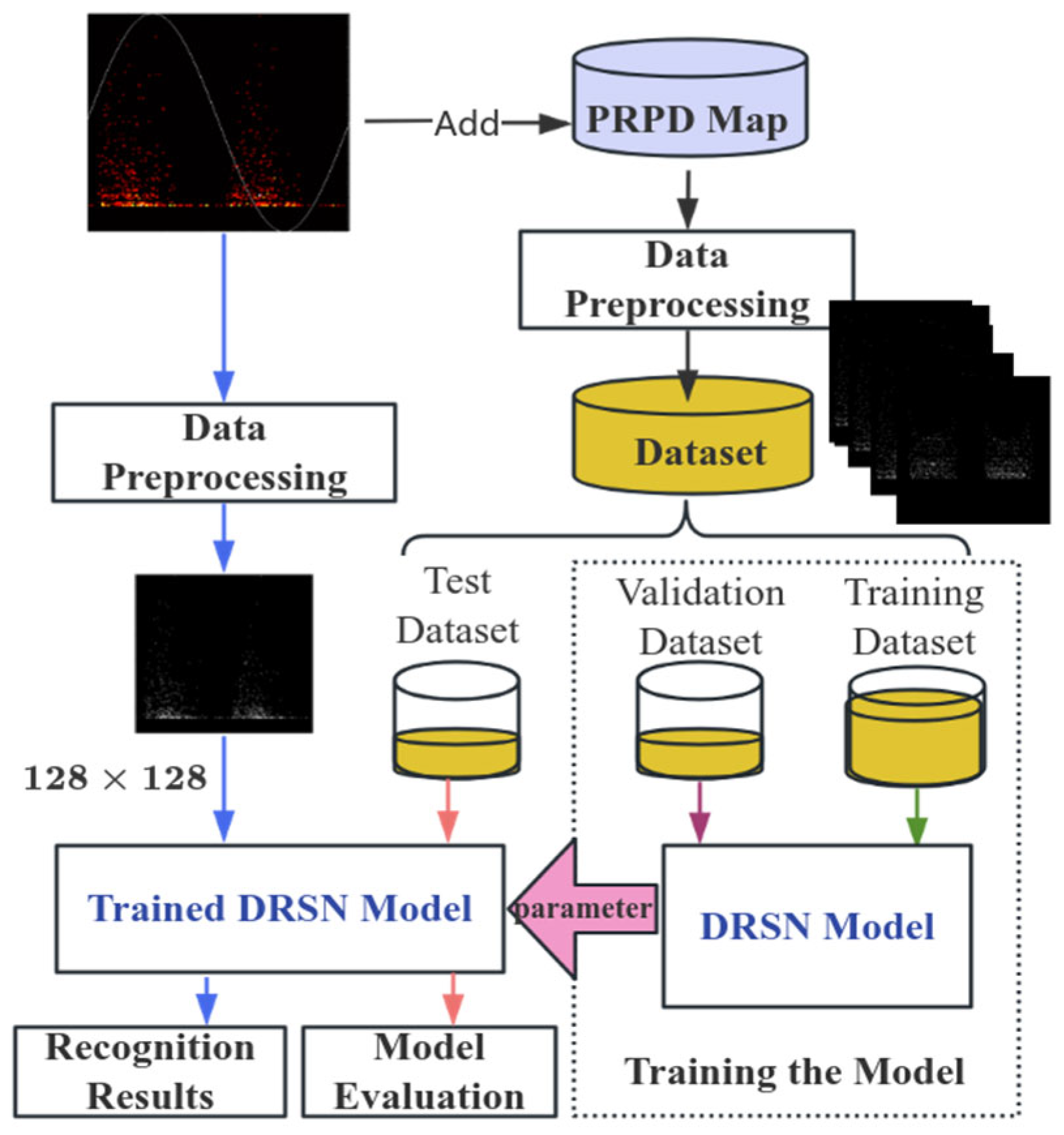
The flowchart of the DRSN-based transformer partial discharge recognition algorithm is shown in Figure 5. The key steps are as follows:
(1)
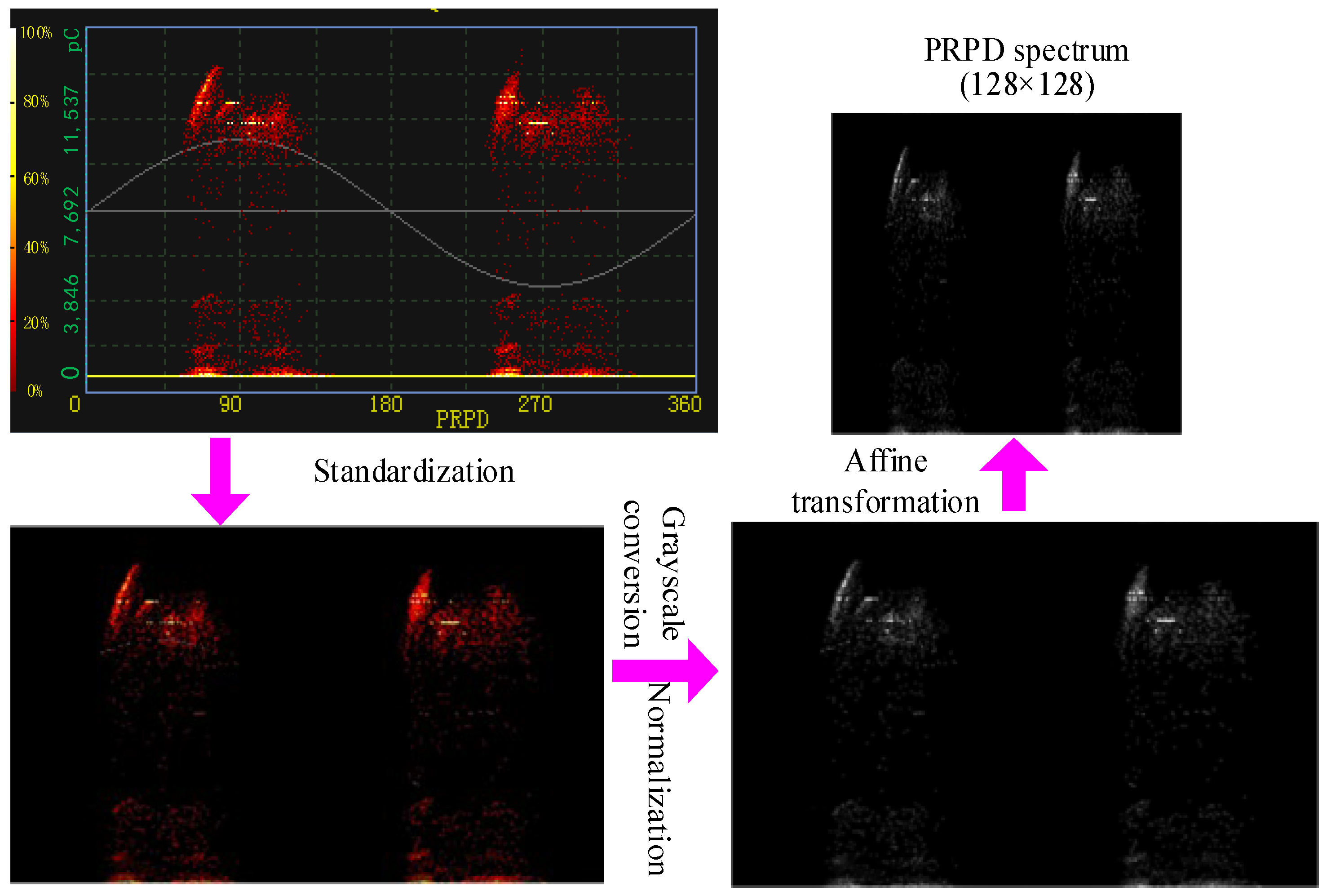
PRPD image preprocessing: The display color and pixel resolution of PRPD images vary among different types of PD analyzers, and auxiliary information such as grid lines and phase reference sine lines in the images can interfere with PRPD pattern recognition. To address this, the collected or sorted PRPD images are preprocessed by removing auxiliary information, converting them to 128 × 128 grayscale images, and normalizing pixel values to the [0, 1] range. Subsequently, data augmentation techniques are applied, and noise is added to enhance dataset diversity and model robustness.
(2)
Model training: DRSN model parameters are trained using the raining dataset, and its hyperparameters are selected with validation dataset.
(3)
Model evaluation: the trained model is evaluated based on the test dataset.
(4)
Model application: Perform the pattern recognition on the preprocessed PRPD image to be tested.

4. Experimental Results and Analysis

4.1. Experimental Dataset Construction

4.1.1. PRPD Data Acquisition

Acquiring and constructing a partial discharge (PD) dataset is a prerequisite for constructing a partial discharge recognition model. The experiment was carried out on a partial discharge test platform designed by Baoding Tianwei Xinyu Technology Development Co., Ltd. (Baoding, China), as shown in Figure 6. The experiment was conducted on an oil-immersed 35 kV transformer model TWTM-35, which is a three-phase, three-winding transformer with a rated frequency of 50 Hz and rated voltages of 35/0.4/0.4 kV. Four typical PD defect models were set up: tip discharge, surface discharge, air-gap discharge, and floating discharge. A TWHCT-8033K high-frequency current transformer (HFCT) was used to collect partial discharge signals from the neutral grounding wire of the transformer winding. The signals were detected by a TWPD-2F comprehensive partial discharge analyzer, with a sampling rate of 20 MS/s, a bandwidth range of 10 kHz to 20 MHz, and a measurement range of 0.1 pC to 10,000 pC.
During the experiment, the transformer was powered by a voltage regulation platform and energized through the low-voltage winding. The voltage regulation platform has a rated input of three-phase AC 380 V and an output of three-phase AC voltage ranging from 0 to 400 V. The experiment employed a gradient step-up method, starting from a lower voltage level and gradually increasing the voltage applied to the low-voltage winding of the transformer until characteristic partial discharge defects was triggered and stably observed. The partial discharge analyzer was set to generate one PRPD after collecting discharge signals for every 2 s, corresponding to 100 power frequency cycles.
Figure 7 shows the collected PRPD examples for four types of partial discharge. The horizontal axis of the image represents the discharge phase (0~360°), the vertical axis shows the normalized discharge quantity, and the values in the matrix indicate the number of partial discharges at the corresponding phase and quantity bins.
It is evident that PRPD patterns of different partial discharge types exhibit distinct characteristic differences.
For tip discharge defects, the discharge pulse phases are mainly distributed near the applied voltage peak, and the discharge signal displays a polarity effect. Surface discharges mainly occur near the rising edge and peak values of both the positive and negative half cycles, with a wide phase distribution and a less obvious polarity effect. Air gap discharges primarily occur within the phase ranges of 0–90° and 180–270°, with positive and negative half cycles showing similar discharge amplitudes and counts. The floating discharge phases are mainly distributed on both sides of the applied voltage peak, exhibiting some symmetry between positive and negative half-cycles, with a relatively strip-shaped distribution area.
The number of PRPD samples collected in the experiment is 490, 310, 200 and 370 for tip discharge, surface discharge, air gap discharge and floating discharge, respectively. The PRPD images were preprocessed to generate original 128 × 128 grayscale images, thereby constructing the original dataset.

4.1.2. Sample Expansion

Image recognition based on deep learning typically requires a large volume of image data as model input. However, the limited number of PRPD obtained from partial discharge tests, especially when derived from highly repeatable laboratory measurements free from noise interference, poses a significant challenge. Models trained on such data exhibit weak generalization ability, struggling to adapt to the complexities of partial discharge pattern recognition in real-world engineering scenarios, which involve intricate insulation structures and complex electromagnetic environments. To enhance model’s robustness and practical applicability, it is therefore necessary to augment the PRPD sample data through techniques including data augmentation and the addition of simulated noise [23,24].
(1)
Data augmentation
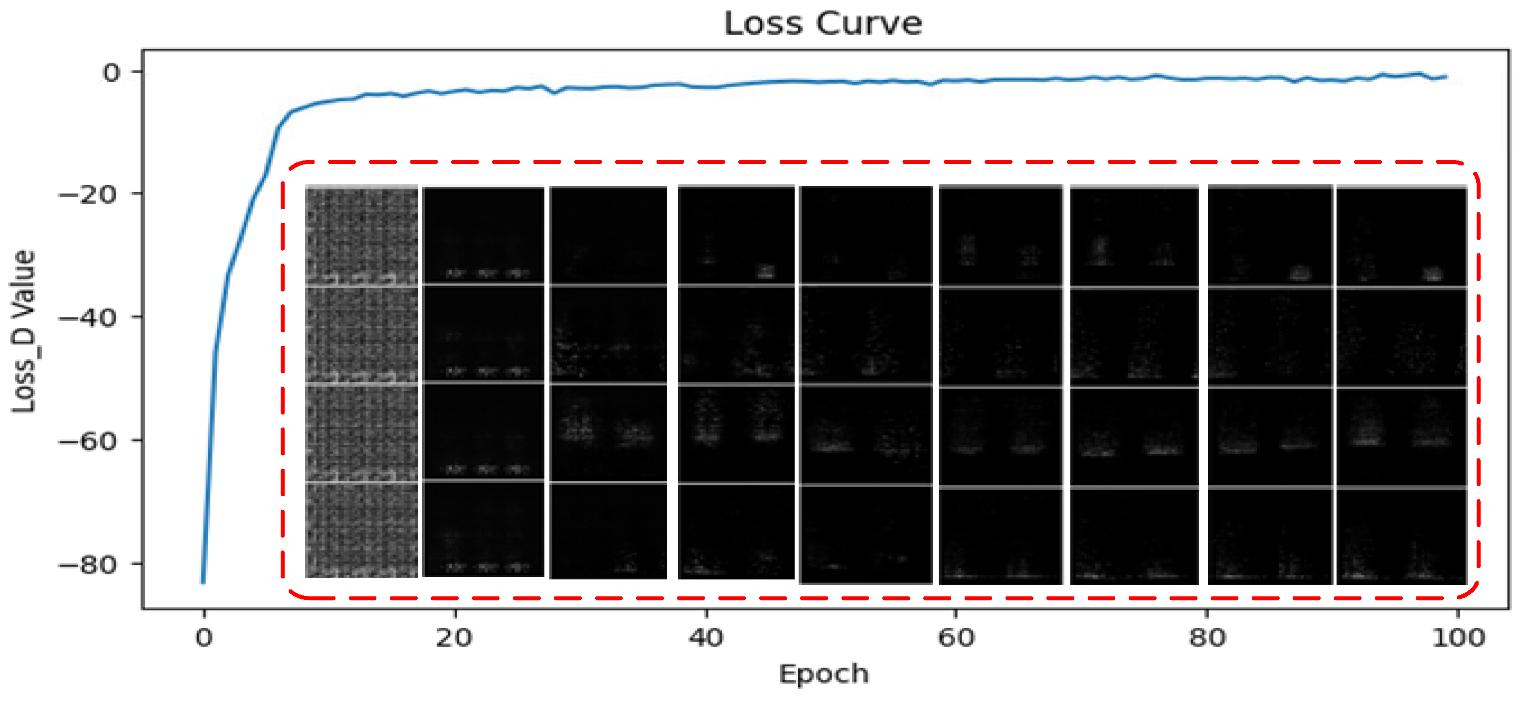
The original PRPD dataset was expanded using the Wasserstein GAN with Gradient Penalty (WGAN-GP). As shown in Figure 8, the adversarial loss function of the generator exhibits a stable convergence trend during the training process. With an increasing number of iterations, the generator gradually captures the implicit distribution characteristics of the discharge pulses. Consequently, the distribution features in the generated samples become more pronounced, and the clarity of the spectral textures is progressively refined. After 100 epochs, the loss value stabilizes, indicating the completion of the training process. The number of PRPD samples for each type of discharge defect was augmented to 800, resulting in an enhanced and balanced dataset.
(2)
Noise simulation
In practical engineering, transformers operate within complex electromagnetic environments characterized by significant noise interference. To improve the generalization ability of the model, it is necessary to introduce artificial noise into the PRPD experimental dataset. During the partial discharge detection of substation transformer, the PRPD images is susceptible to three typical types of electromagnetic interference, including random white noise arising from the inherent characteristics of the circuit, periodic noise caused by power frequency and harmonic interference, and impulse noise from switch operation or electromagnetic wave signal. This paper injects these above noise types into the sample set to simulate the impact of actual electromagnetic interference on the spectrum, thereby enhancing the robustness of the model and better adapting to practical applications. Examples of the injected noise spectrum are shown in Figure 9, and the resulting datasets are shown in Table 2.

4.2. Experimental Results Analysis

The DRSN model was implemented using the Pytorch framework (version 2.6.0). The dataset is split into training/validation dataset and the test dataset at an 8:2 ratio. Model parameters are updated using the stochastic gradient descent (SGD) optimizer. The model hyperparameters were determined by grid search. The number of training epochs is set to 50, the batch size is 32, the learning rate is dynamically adjusted using StepLR with a decay factor is 0.5, and the loss function focus parameter γ is 2. For comparison, the partial discharge recognition models based on classic CNNs were constructed, including AlexNet, VGG-16 and ResNet18. The input and output layers of these conventional models are modified to suit the specific requirements of the recognition task. These models are trained using the Adam optimizer and cross entropy loss function. All training is conducted on a server featuring an NVIDIA T4 GPU, with 12.67 GB system memory and 16 GB GDDR6 video memory.

4.2.1. Effectiveness Analysis of Feature Extraction

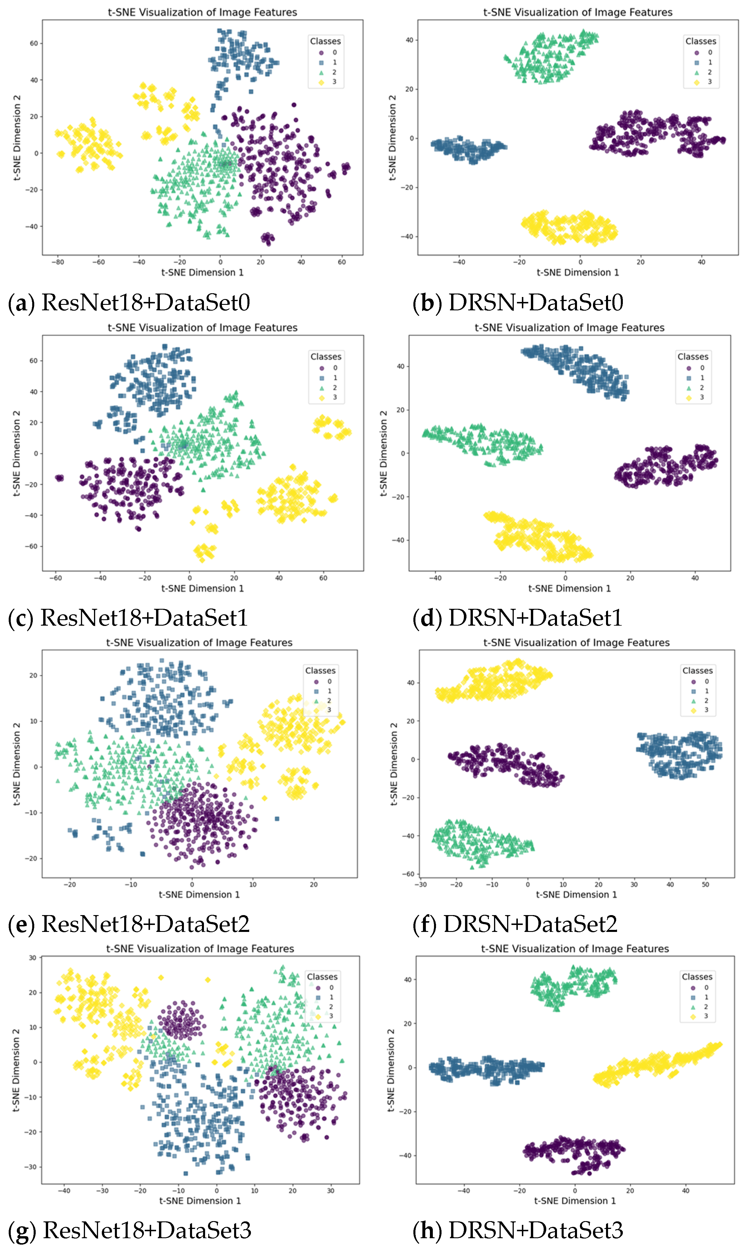
The feature extraction capability of the model is critical to achieving accurate discharge type identification. The features extracted by the proposed DRSN model and the baseline CNN models are analyzed across three datasets: the original dataset, augmented dataset and the noisy datasets. For ease of observation, the input features to the classification layer are reduced using the t-SNE method and then visualized. Figure 10 shows the visualization results of the features extracted by the DRSN model and the ResNet18 model.
The visualization results of feature extraction on the original PRPD dataset (DataSet0) show that the features extracted by the DRSN model exhibit high intra-class compactness and clear inter-class separation. In contrast, features extracted by the ResNet18 model show loose intra-class clustering, class overlap, and the presence of outliers. The feature visualization results of the augmented dataset DataSet1 are similar to those of DataSet0, with the ResNet18 model showing slightly better inter-class separability on DataSet1 compared to the imbalanced dataset DataSet0.
The feature visualization results for the noisy datasets (DataSet2 and DataSet3), demonstrate that the features extracted by the DRSN model still show excellent intra-class compactness and inter-class separation. This indicates that the model’s feature extraction is robust to noise and maintains good representation capabilities for noise data; in contrast, the ResNet18 model’s feature extraction under noisy conditions results in significantly reduced inter-class separation and blurred class boundaries, particularly in mixed noise datasets, leading to substantial inter-class confusion and an increased risk of misclassification.
Experimental results demonstrate that the proposed DRSN model possesses strong feature representation capability on both original and noisy datasets, significantly outperforming conventional CNN models in terms of class discrimination and noise robustness.

4.2.2. Discharge Pattern Recognition Performance Analysis

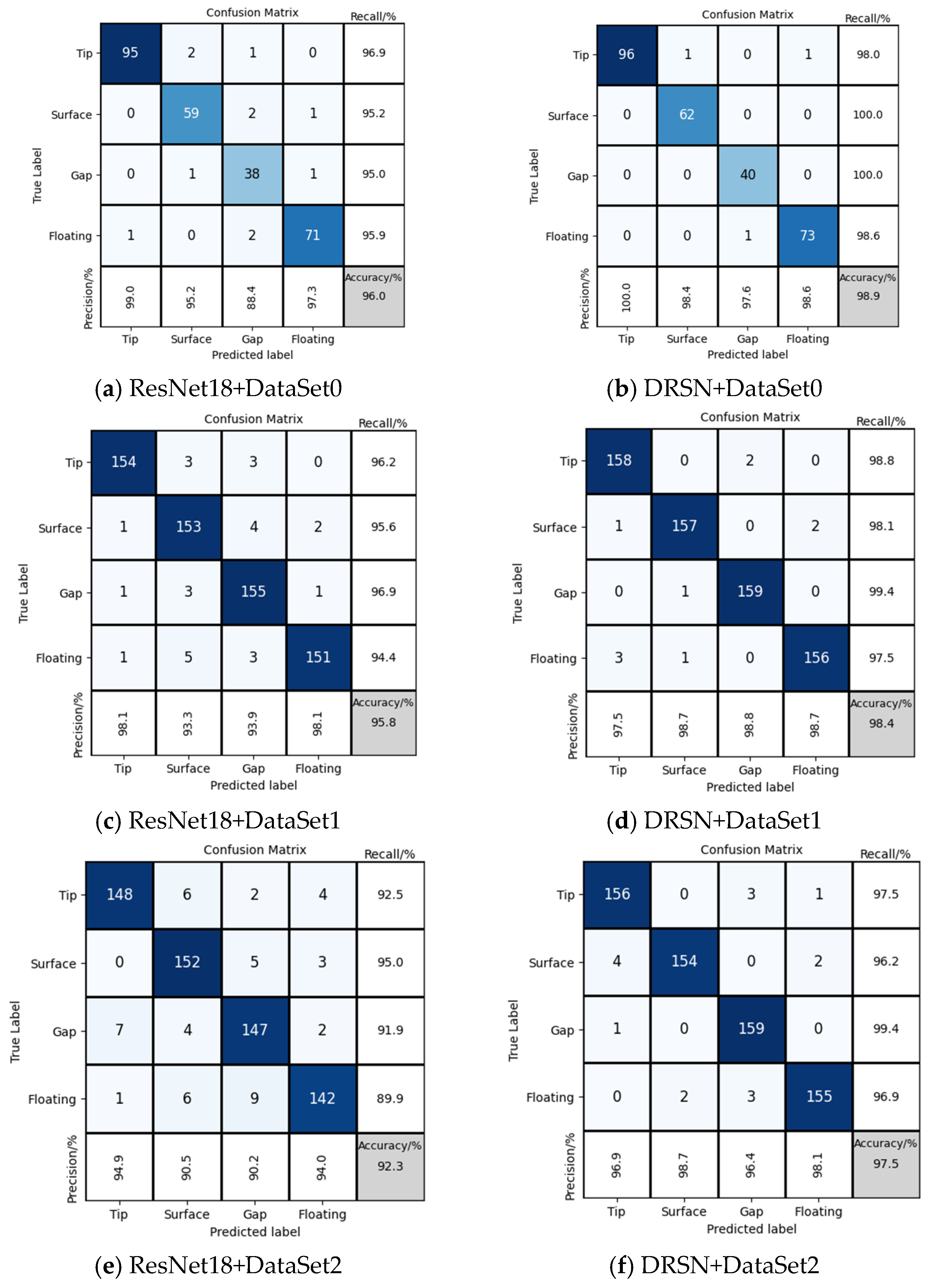
The proposed DRSN model and the conventional CNN models are applied to the discharge pattern recognition task on both the original dataset and the noisy datasets. Figure 11 shows the confusion matrices for the ResNet18 model and DRSN model on the test dataset. In each matrix, the horizontal axis denotes the true labels of each discharge type, while the vertical axis represents the recognition result by the model. The values in the matrix represent the number of samples classified into each class by the model, with the diagonal values indicating correctly recognized samples and the off-diagonal values representing misclassified samples.
As illustrated in the figure, the DRSN model misclassifies significantly fewer samples than ResNet18 across the original, augmented, and various noisy datasets. Precision and recall rates of DRSN model for each discharge type are consistently maintained above 94%. In contrast, ResNet18 exhibits a substantial increase in misclassified samples and a significant decrease in precision and recall rates when dealing with noisy datasets, particularly those with mixed noise.
Table 3 shows the comparison of different models’ discharge pattern recognition accuracy on both original and noisy datasets. The accuracy values are the average accuracy rates obtained from 5-fold cross-validation.
Experimental results demonstrate that the proposed DRSN model has significantly higher recognition accuracy than the conventional CNN models. On both the original and enhanced datasets, DRSN model has an accuracy exceeding 98.0%, marking an improvement of 2.4 to 4.2% over the benchmark models. Furthermore, on the noisy dataset, the DRSN model maintains an accuracy exceeding 96%, outperforming the benchmark models noticeably. Notably, on the mixed-noise dataset, it achieves significantly higher accuracy compared to traditional models, highlighting its superior robustness to noise.
The average inference time of the DRSN model for recognizing a single sample is 69.7 milliseconds in a GPU-based training environment. On a general-purpose computer equipped with an Intel® Core™ i7-8700 CPU, 16.0 GB of RAM, and running the 64-bit Windows 10 operating system, the average inference time is 616.4 milliseconds, which satisfies the requirements for rapid diagnosis.

4.2.3. Noise Immunity Analysis

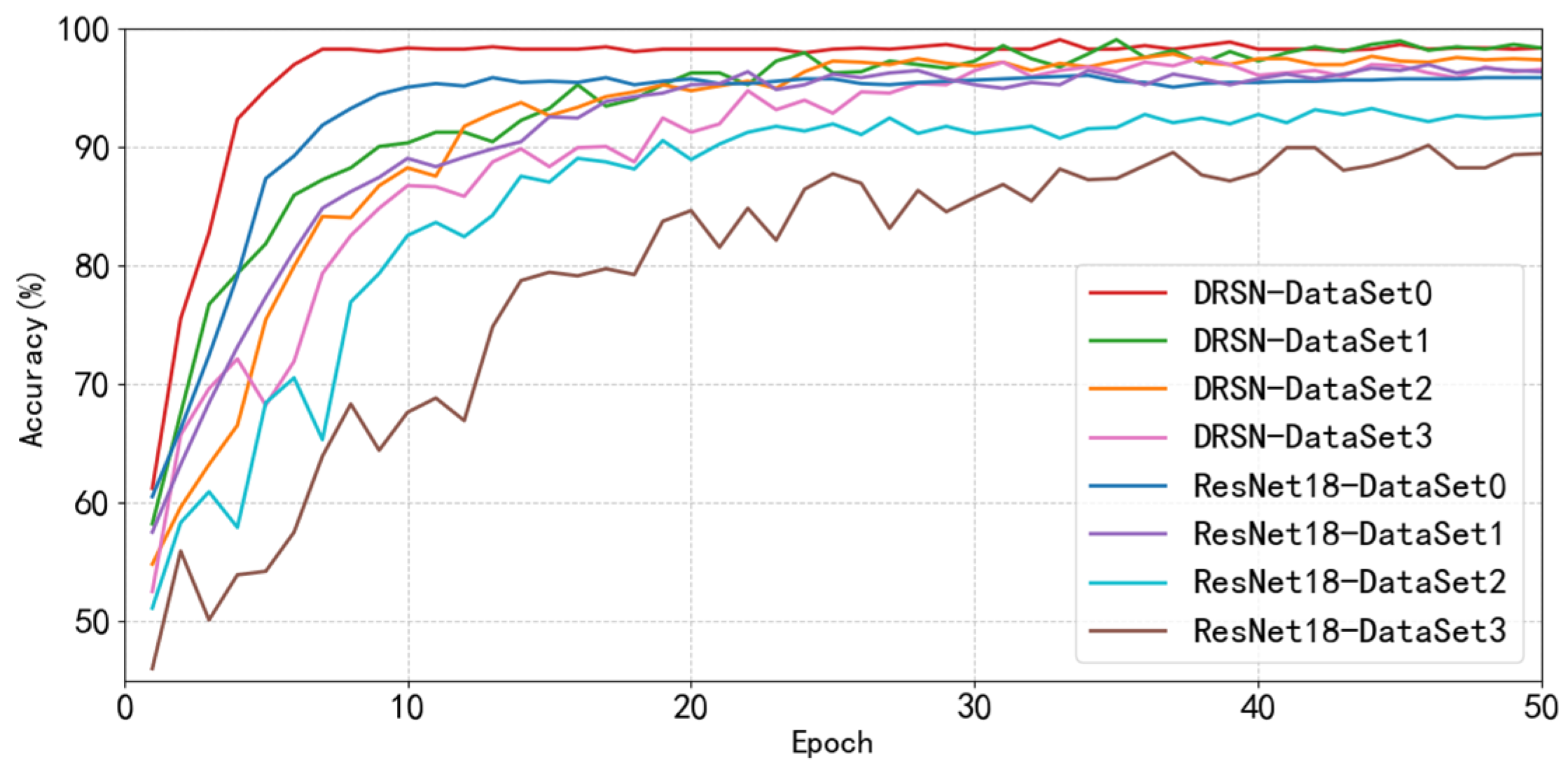
To further evaluate the model’s performance under different noise interference, Figure 12 shows the test accuracy curves of the DRSN model and the ResNet18 model across the training epochs on four PRPD pattern datasets.
AS shown in Figure 12, the DRSN model rapidly achieves an accuracy exceeding 96% within 30 iterations on the original dataset, the enhanced dataset, and the datasets with different noise interference. The accuracy and stability on both Gaussion noise dataset and mixed noise dataset are close to those achieved on the original dataset. In contrast, the accuracy of the RestNet18 model increases slowly and fluctuates significantly under noise interference, particularly on the mixed noise dataset. Although its accuracy improves with iterations, its accuracy is still only maintained in a fluctuation range of 85–90% even after more than 30 iterations, which is significantly lower than that of the DRSN model. These results demonstrate that the proposed DRSN model has clear advantages in noise immunity, exhibiting stronger noise robustness and improved suitability for accurate identification of transformer partial discharge under complex operating conditions.

4.3. Model Generalization Performance Analysis

The transformer partial discharge conditions simulated in laboratory settings are relatively simple. However, real-world monitoring data is complicated by structural differences among different types of transformers, electromagnetic interference, mechanical vibration, and other external factors, resulting in the diversity of PRPD patterns. Therefore, it is necessary to evaluate the model’s generalization capability in other experimental environments or real application scenarios.
(1)
Case Application 1
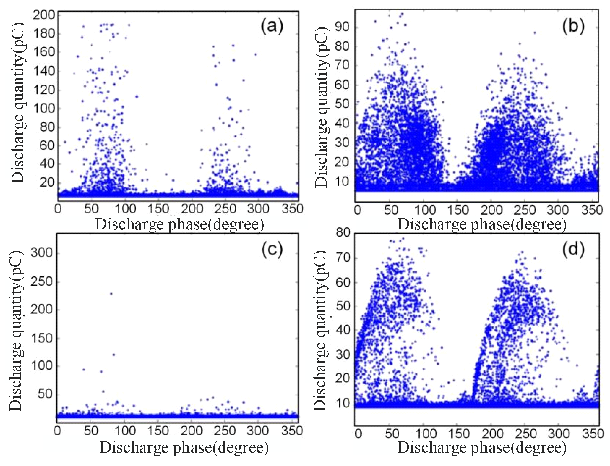
Figure 13 presents the PRPD images of surface discharge phenomena in soybean oil-impregnated insulation paperboard and mineral oil-impregnated insulation paperboard with varying moisture contents under plate-to-plate electrodes, as reported by B.T. Phung from the University of New South Wales, Australia, in 2007 [25,26].
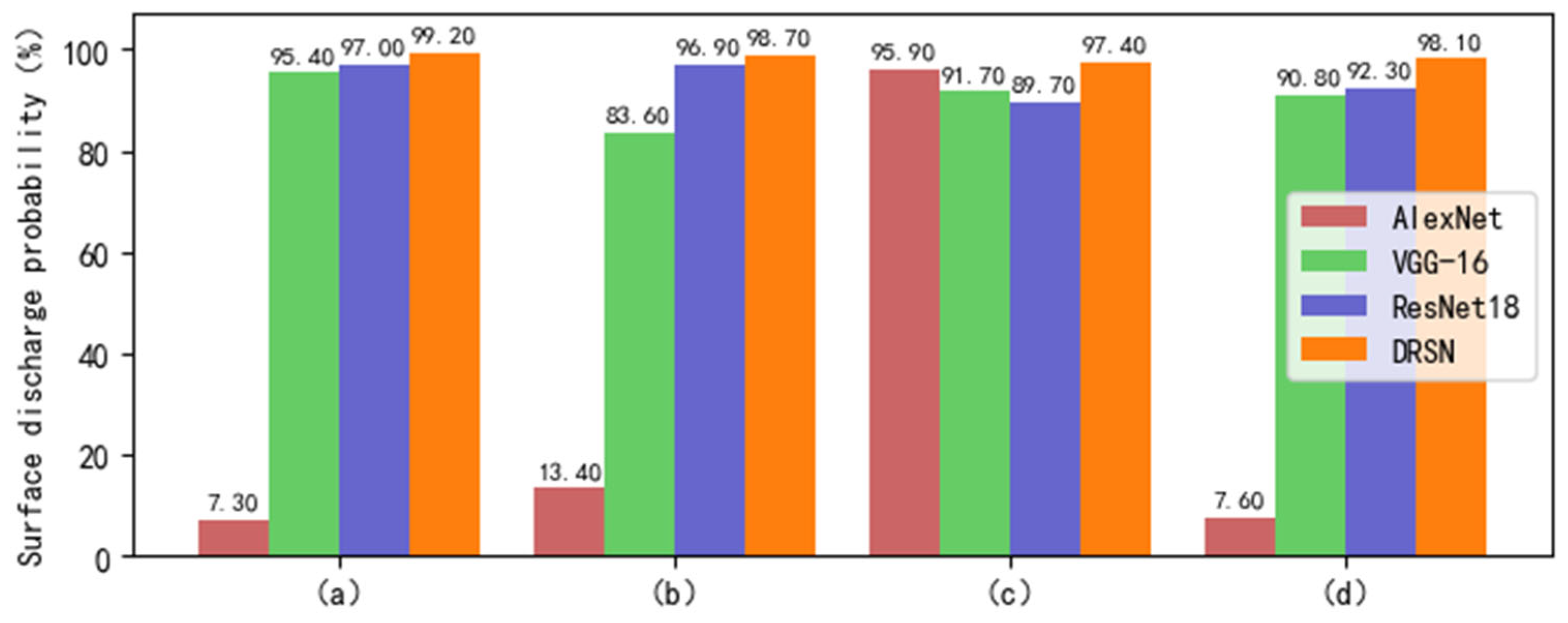
The above PRPD images are preprocessed and converted into 128 × 128 gray-scale images. Subsequently, both the proposed DRSN model and conventional CNN models are employed for pattern recognition. Figure 14 shows the probabilities of each model identifying the PRPD images as surface discharge.
Comparing the PRPD images in Figure 13, it is evident that the pulse amplitude and pulse count of surface discharge show significant differences under different working conditions. As shown in Figure 14, VGG-16, ResNet18 and the proposed DRSN model all successfully recognize the discharge pattern. The deep learning method demonstrates superior generalization capability in transformer PRPD pattern recognition. This advantage stems from its ability to overcome the limitations of traditional machine learning methods, which rely on predefined features such as pulse amplitude and pulse count. Instead, deep learning models can directly learn and extract complex features from PRPD images, such as the distribution shapes reflecting the discharge pattern, making their recognition results less susceptible to variations in experimental devices, sample collection duration, sampling frequency, discharge development stage, or the on-site operating environment.
Furthermore, the DRSN model consistently achieves recognition probabilities above 97% for identifying the four PRPD images as surface discharge, outperforming conventional CNN models and demonstrating superior recognition reliability. The results demonstrate that the proposed model has better generalization performance when dealing with discharge phenomena with significant variations in pulse amplitude and pulse count.
(2)
Case Application 2
Figure 15 shows the PRPD and PRPS images collected from an operational transformer using a partial discharge comprehensive analyzer. The type of transformer discharge has been confirmed as floating discharge. Preprocess the PRPD image and convert it into a standardized 128 × 128 grayscale image. The image processing process is shown in Figure 16.
The DRSN recognition model and conventional CNN models are used to identify the discharge type of the image, with the recognition results presented in Figure 17.
As can be seen from Figure 17, the AlexNet and ResNet18 models fail to correctly classify the PRPD, while the VGG-16 and DRSN models achieve accurate classification. The proposed DRSN model achieves a 95.6% probability in predicting a floating discharge, representing a 23.3% improvement over the VGG-16 model. This demonstrates that the DRSN partial discharge recognition model proposed in this paper has better generalization capability compared to conventional CNN models.

5. Conclusions

To address the limitations of traditional deep convolutional neural networks in learning discriminative features and achieving high recognition accuracy when processing partial discharge data under complex operating conditions or in the presence of noise interference, this paper presents an exploratory study on partial discharge identification methods based on deep residual shrinkage networks. The main conclusions are as follows:
(1) A DRSN model for PRPD pattern recognition was developed, incorporating a dual-path feature extraction architecture based on deep residual structures to fuse both local and global features. A channel-wise adaptive soft-thresholding denoising mechanism was introduced to effectively suppress noise interference. In addition, the Focal Loss function was employed to optimize network training by enhancing sensitivity to hard-to-classify samples.
(2) Performance comparison experiments were conducted between the proposed DRSN model and conventional CNN models. The visualization of the dimensionally reduced feature space show that the features extracted by the DRSN model exhibit significantly better inter-class separability than those extracted by conventional CNNs. In addition, the proposed model achieves higher average recognition accuracy on both the original and noise-contaminated datasets. Notably, its discharge recognition accuracy of DRSN model under various types of noise interference remains comparable to that achieved without any noise. The above results demonstrate that the proposed model has superior feature representation capabilities and maintains robust recognition performance in noisy environments.
The dataset for this study was obtained from a transformer test platform by artificially setting partial discharge defect models. It is important to note that the current defect models are relatively simple, and the experimental environment differs from actual field operating conditions in aspects such as electromagnetic interference, temperature, and humidity. These factors may potentially influence the performance of the proposed method in real-world applications. Although we have attempted to validate the model’s generalization capability through cross-scenario cases, the limited number of cases means its effectiveness in practical applications still requires further rigorous testing.
Future research will concentrate on two primary areas: Firstly, enriching the experimental data by incorporating more diverse defect models and recording test parameters in greater detail to enhance the interpretability and practical value of the experimental results; Secondly, actively collecting and organizing partial discharge data from transformers in actual operation to increase the diversity of the dataset, thereby effectively improving the model’s generalization ability and its potential for practical applications.

Author Contributions

Methodology, Y.W. and Y.Z.; software, Y.W.; writing—original draft preparation, Y.W.; writing—review and editing, Y.W. and Y.Z. All authors have read and agreed to the published version of the manuscript.

Funding

This research was funded by the National Natural Science Foundation of China, grant number 51677072 and the Natural Science Foundation of Hebei Province, grant number F2022502002.

Data Availability Statement

The datasets used and/or analyzed during the current study are available from the corresponding author on reasonable request.

Conflicts of Interest

The authors declare no conflicts of interest.

References

  1. IEEE Std C57.127-2018; Guide for the Detection and Location of Acoustic Emissions from Partial Discharges in Oil-Immersed Power Transformers. IEEE: New York, NY, USA, 2018.
  2. Shang, H.; Zhang, R.; Huang, T.; Lin, W.; Zhao, Z. Partial discharge signal denoising based on CEEMDAN-TQWT method for power transformers. J. Electr. Power Sci. Technol. 2024, 39, 272–284. [Google Scholar]
  3. Jiang, Y.; Zhu, Y.; Jiang, X.; Wan, Y. Partial discharge noise suppression method based on improved LMS Adaptive Filtering. Sci. Technol. Eng. 2022, 22, 1039–1047. [Google Scholar]
  4. Cheng, Y.; Zhang, Z. Multi-source partial discharge diagnosis of transformer based on Random Forest. Proc. CSEE 2018, 38, 5246–5256+5322. [Google Scholar]
  5. Kong, X.; Cai, B.; Yu, Y.; Yang, J.; Wang, B.; Liu, Z.; Shao, X.; Yang, C. Intelligent diagnosis method for early faults of electric-hydraulic control system based on residual analysis. Reliab. Eng. Syst. Saf. 2025, 261, 111142. [Google Scholar] [CrossRef]
  6. Zhang, J.; Wu, N.; Wang, Y.; Ma, Z.; Li, X.; Liu, C.; Wu, G. Partial discharge development process of oil-immersed aramid paper based on dynamic change rate of discharge statistical parameters. Insul. Mater. 2022, 55, 72–77. [Google Scholar]
  7. Dang, X.; Huang, R.; Liu, S.; Huang, Z. Analysis of single-pulse waveform of partial discharge based on time-frequency characteristics. Electr. Meas. Instrum. 2019, 56, 52–56. [Google Scholar]
  8. Chen, J.; Xu, C.; Li, P.; Shao, X.J.; Li, C.L. Feature extraction method for partial discharge pattern in GIS based on time-frequency analysis and fractal yheory. High Volt. Eng. 2021, 47, 287–295. [Google Scholar]
  9. Wang, L.; Chu, M.; Wang, X.; Guan, H.; Chen, P.; Gao, G. Research on monitoring method of primary equipment operation state in intelligent substation based on random forest. Electr. Meas. Instrum. 2024, 61, 184–190. [Google Scholar]
  10. Yao, R.; Hui, M.; Li, J.; Bai, L.; Wu, Q. Feature extraction and optimal selection based on Random Forest for partial discharges. J. North China Electr. Power Univ. 2021, 48, 63–72. [Google Scholar]
  11. Ren, M.; Xia, C.; Chen, R. Multispectral ratio characteristics analysis of partial discharge. Proc. CSEE 2023, 43, 809–819. [Google Scholar]
  12. Fan, L.; Lu, Y.; Tao, F. Application of artificial intelligence in partial discharge detection partⅡ: Pattern recognition and condition assessment. Insul. Mater. 2021, 54, 10–24. [Google Scholar]
  13. Hinton, G.E.; Osindero, S.; The, Y.W. A fast learning algorithm for deep belief nets. Neural Comput. 2006, 18, 1527–1554. [Google Scholar] [CrossRef]
  14. LeCun, Y.; Bengio, Y.; Hinton, G. Deep learning. Nature 2015, 521, 436–444. [Google Scholar] [CrossRef]
  15. Zhou, X.; Zhu, H.; Ma, Y. Partial discharge pattern recognition of transformer based on Deep Learning. High Volt. Appar. 2019, 55, 98–105. [Google Scholar]
  16. Zhang, Y.; Zhu, Y. A partial discharge pattern recognition method combining graph signal and graph convolutional network. Proc. CSEE 2021, 41, 6472–6481. [Google Scholar]
  17. Yang, C.; Wang, M.; Zhao, S.; Wu, N.; Dong, Q.; Cui, J.; Han, X. Research on partial discharge diagnosis algorithm for high voltage cable based on Deep Learning fusion method. High Volt. Appar. 2023, 59, 65–73. [Google Scholar]
  18. Chen, J.; Zhou, Y.; Bai, Z.; Zhao, Y. Pattern recognition method of partial discharge in oil-paper insulation based on multi-channel Convolutional Neural Network. High Volt. Eng. 2022, 48, 1705–1715. [Google Scholar]
  19. Xu, C.; Chen, J.; Liu, W.; Lv, Z.; Li, P.; Zhu, M. Pattern recognition of partial discharge PRPD Spectrum in GIS based on Deep Residual Network. High Volt. Eng. 2022, 48, 1113–1123. [Google Scholar]
  20. Lu, F.; Liu, G.; Wang, Q.; Lu, X.; Ou, Q.; Wang, S. Research on transformer partial discharge fault diagnosis method based on improved Residual Network and InforGAN. J. North China Electr. Power Univ. 2024, 51, 10–19. [Google Scholar]
  21. Tang, Z.; Cao, Z.; He, N. Application of Convolutional Neural Network transfer learning in partial discharge type diagnosis. High Volt. Appar. 2022, 58, 158–164. [Google Scholar]
  22. Zhao, M.; Zhong, S.; Fu, X.; Tang, B.; Pecht, M. Deep residual shrinkage networks for fault diagnosis. IEEE Trans. Ind. Inform. 2020, 16, 4681–4690. [Google Scholar] [CrossRef]
  23. Shao, X.; Cai, B.; Zou, Z.; Liu, Y.; Shao, H.; Yang, C. Artificial intelligence enhanced fault prediction with industrial incomplete information. Mech. Syst. Signal Process. 2025, 224, 112063. [Google Scholar] [CrossRef]
  24. Chen, H.; Guo, W.; Kang, K.; Hu, G. Automatic Modulation Recognition Method Based on Phase Transformation and Deep Residual Shrinkage Network. Electronics 2024, 13, 2141. [Google Scholar] [CrossRef]
  25. Imamovic, D.; Lai, K.X.; Muhamad, N.A.; Phung, T.; Blackburn, T. Partial discharge and dissolved gas analysis in biodegradable transformer oil. In Proceedings of the CIGRÉ Colloquium, Brugge, Belgium, 1 January 2007; pp. 1–7. [Google Scholar]
  26. Cui, L. Study on Discharge Characteristics and Its Effect on Insulation Detorioration of Thermal-Aged Vegetable Oil-Paper Insulation; Chongqing University: Chongqing, China, 2018. [Google Scholar]
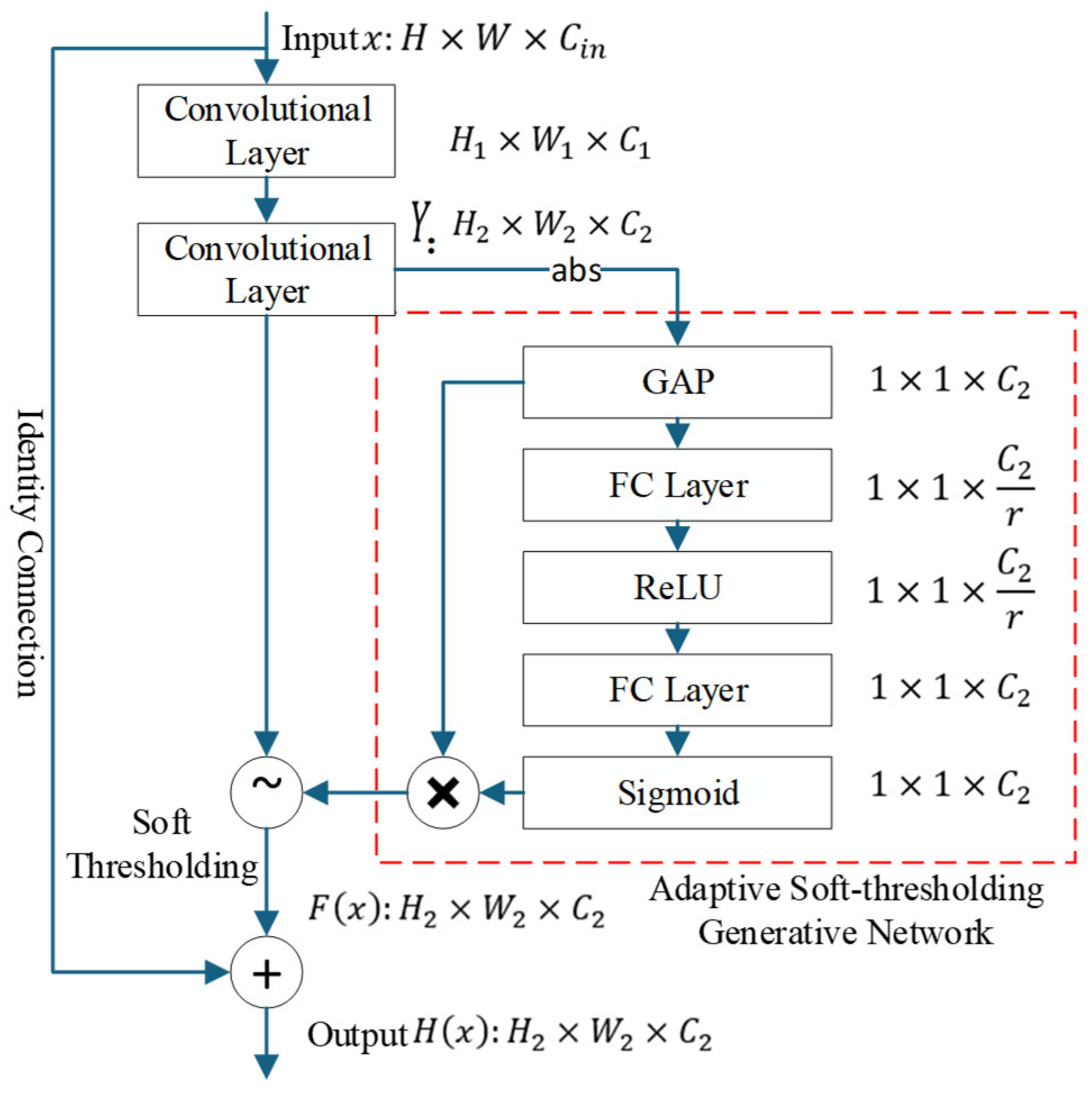
Figure 1. RSB structure.
Electronics 14 03181 g001
Figure 2. Example of convolution, batch normalization and activation.
Electronics 14 03181 g002
Figure 3. The relationship between input and output in Soft Thresholding.
Electronics 14 03181 g003
Figure 4. Network structure of DRSN model.
Electronics 14 03181 g004
Figure 5. Flowchart of partial discharge recognition algorithm.
Electronics 14 03181 g005
Figure 6. Partial discharge test.
Electronics 14 03181 g006
Figure 7. Examples of PRPD under different discharge types.
Electronics 14 03181 g007
Figure 8. Training loss curve of WGAN-GP and examples of generated images.
Electronics 14 03181 g008
Figure 9. Examples of PRPD with different types of noise added.
Electronics 14 03181 g009
Figure 10. Visualization of t-SNE features for different models and datasets.
Electronics 14 03181 g010
Figure 11. Confusion matrix of ResNet18 and DRSN.
Electronics 14 03181 g011aElectronics 14 03181 g011b
Figure 12. Test accuracy curves under conditions of different noise levels.
Electronics 14 03181 g012
Figure 13. PRPD of surface discharge: (a) Dry mineral oil-impregnated insulation paperboard, 1.5 mm thick, at 19 kV; (b) Dry soybean oil-impregnated insulation paperboard, 1.5 mm thick, at 18 kV; (c) Wet mineral oil-impregnated insulation paperboard, 3 mm thick, at 25 kV; (d) Wet soybean oil-impregnated insulation paperboard, 3 mm thick, at 29 kV.
Electronics 14 03181 g013
Figure 14. PRPD recognition result: (a) Probability of PRPD in Figure 13a identified as surface discharge by models; (b) Probability of PRPD in Figure 13b identified as surface discharge by models; (c) Probability of PRPD in Figure 13c identified as surface discharge by models; (d) Probability of PRPD in Figure 13a identified as surface discharge by models.
Electronics 14 03181 g014
Figure 15. Example of on-site floating discharge.
Electronics 14 03181 g015
Figure 16. Preprocessing process of PRPD.
Electronics 14 03181 g016
Figure 17. Partial discharge recognition results based on different methods.
Electronics 14 03181 g017
Table 1. Structure and parameters of DRSN model.
LayerKernel/Stride/ChannelsOutput Dimension
Input--128 × 128 × 1
Conv2d+BN+ReLU7 × 7/2/6464 × 64 × 64
MaxPool2d3 × 3/2/--32 × 32 × 64
Stage 1:
Standard RSB × 23 × 3/1/64-6432 × 32 × 64
Stage 2:
Downsampling RSB3 × 3/2/12816 × 16 × 128
Standard RSB3 × 3/1/12816 × 16 × 128
Stage 3:
Downsampling RSB3 × 3/2/2568 × 8 × 256
Standard RSB3 × 3/1/2568 × 8 × 256
Stage 4:
Downsampling RSB3 × 3/2/5124 × 4 × 512
Standard RSB3 × 3/1/5124 × 4 × 512
GlobalAvgPool--1 × 1 × 512
FC+Softmax--4
Table 2. Summary of datasets.
NameDescribe
DataSet0Original experimental PRPD dataset
DataSet1Dataset augmented by WGAN-GP
DataSet2Gaussian white noise to DataSet1: the mean is 0 and the standard deviation is randomly between 0.05–0.20
DataSet3Three types of noise are injected into DataSet1 with equal probability: Gaussian white noise, periodic noise and impulse noise
Table 3. Comparison of different models’ partial discharge recognition performance.
ModelDataSet0DataSet1DataSet2DataSet3
AlexNet94.5%94.0%91.1%88.5%
VGG-1693.8%94.4%89.7%86.3%
ResNet1895.6%95.9%92.4%89.4%
DRSN98.0%98.1%97.2%96.2%
Disclaimer/Publisher’s Note: The statements, opinions and data contained in all publications are solely those of the individual author(s) and contributor(s) and not of MDPI and/or the editor(s). MDPI and/or the editor(s) disclaim responsibility for any injury to people or property resulting from any ideas, methods, instructions or products referred to in the content.