Accelerating Broadband DOA Estimation: A Real-Valued and Coherent Sparse Bayesian Approach for 5G Sensing

Abstract

For applications like smart cities and autonomous driving, high-precision direction-of-arrival (DOA) estimation for 5G broadband signals is essential. A primary obstacle for existing methods is the spatial incoherence caused by multi-frequency propagation. We present a sparse Bayesian learning (SBL) algorithm specifically designed to resolve this issue while also minimizing computational load. The algorithm synergistically combines three key components: first, a multiple-signal classification (MUSIC)-like focusing technique ensures a coherent sparse model; second, a real-valued transformation significantly cuts down on computational complexity; and third, an optimized variational Bayesian inference accelerates convergence via root-finding. Validation against MUSIC and rootSBL confirms our method’s marked superiority in low-SNR, limited-snapshot, and multipath conditions delivering both higher accuracy and faster convergence. This work, thus, contributes an effective and practical solution for real-time 5G DOA sensing.

1. Introduction

The study of 5G signal sensing, particularly in the context of integrated sensing and communication (ISAC), holds significant importance for modern wireless systems where there is increasing demand for high-precision positioning and DOA estimation. Leveraging its high-speed transmission, large bandwidth, and low-latency characteristics, 5G technology not only enhances data transmission efficiency but also enables high-precision positioning and real-time tracking in various applications, including smart cities, autonomous driving, unmanned aerial vehicle navigation, and industrial Internet of Things (IoT). For these application scenarios, accurate DOA estimation represents a fundamental requirement, as it directly impacts a system’s ability to identify and determine target locations, movement directions, and signal source positions.

With their extensive spectral resources, 5G broadband signals demonstrate significantly improved anti-interference capabilities and positioning accuracy in complex multipath propagation and high-interference environments. However, conventional narrowband DOA estimation algorithms face substantial challenges when processing broadband signals, including high computational complexity and difficulties in maintaining spatial information consistency. Consequently, the development of efficient DOA estimation algorithms specifically designed for 5G broadband signals becomes critically important.

DOA estimation has been extensively studied for decades, with numerous classical algorithms being developed and refined. Since the 1980s, subspace-based DOA estimation algorithms have emerged as particularly influential approaches. Notable examples include MUSIC, ESPRIT (estimation of signal parameters via rotational invariance techniques), and PUMA (propagator method using modified array) [1,2,3]. These algorithms achieve direction estimation by exploiting the covariance matrix of array outputs, demonstrating near-optimal performance under appropriate conditions, as follows: sufficient signal-to-noise ratio (SNR), known number of signal sources, and adequate snapshots.

In practical spatial scenarios, the complex and dynamic propagation environment often results in multipath signal reception at the receiver, significantly degrading the performance of conventional subspace-based array direction-finding algorithms. To address multipath interference, Shan et al. [4] proposed a spatial-smoothing (SS) decorrelation algorithm based on a uniform linear array (ULA) configuration. This approach divides the ULA into multiple overlapping subarrays with identical array manifolds and then performs weighted averaging of the subarray covariance matrices to obtain a smoothed matrix for subsequent subspace-based DOA estimation. However, traditional subspace methods exhibit significant performance limitations when dealing with limited snapshots or unknown source numbers, making them unsuitable for complex real-world scenarios.

Recent years have witnessed remarkable advances in deep learning (DL) approaches for DOA estimation [5,6,7,8,9,10]. Various neural network architectures have been explored: Cong et al. [11] developed a CNN-based robust estimation method for non-ideal scenarios; ResNet was adapted for near-field DOA estimation [12]; and Wu et al. [13] combined Toeplitz prior with CNN to mitigate grid mismatch effects. However, these methods were not specifically designed for coherent DOA estimation. While Hoang and Lee’s [14] full Toeplitz matrix reconstruction (FTMR) algorithm demonstrated promising results, it fails at SNRs below −10 dB. Papageorgiou et al. [15] proposed a low-SNR CNN model capable of partially handling coherent signals, but its required training samples grow combinatorially with increasing signal numbers.

Building upon these efforts, the field continues to evolve with more sophisticated models. Transformer-based architectures [16], for instance, are being investigated to better capture long-range spatial dependencies, while interpretable, end-to-end differentiable frameworks [17] that treat traditional algorithms like beamforming as learnable neural network layers are also gaining traction. Nevertheless, despite DL’s superior performance in certain aspects of wideband DOA feature extraction, the “black-box” nature of many models remains a significant concern for high-reliability applications.

Sparse representation (SR) has become a prevalent technique for DOA estimation, owing to its enhanced noise robustness and reliable performance under limited snapshots or unknown source numbers [18,19,20,21,22,23]. Among these developments, Malioutov et al. [23] proposed the ℓ₁-SVD algorithm that employs singular value decomposition (SVD) on sensor measurement matrices. This method achieves the following: (1) sparsity enhancement via $l_1$-norm regularization, (2) complexity reduction through SVD processing, and (3) improved noise resistance.

To integrate prior knowledge and Bayesian principles into sparse representation (SR) techniques, sparse Bayesian learning was proposed for DOA and signal amplitude estimation. Compared with conventional SR methods, SBL enhances signal sparsity and exhibits fewer local optima than ℓ₁-norm-based approaches, demonstrating better adaptability to highly correlated manifold matrices in beamforming models. As a result, SBL has been widely applied to DOA and signal amplitude estimation in both single-snapshot and multi-snapshot scenarios [24].

Building upon this framework, Pan et al. [25] utilized variational Bayesian learning (VBL) to approximate posterior distributions by learning hidden parameters, thereby accelerating the estimation process. Wang et al. [26] adopted generalized double Pareto (GDP) priors, which induce stronger sparsity than Laplacian priors, for sparse signal modeling. For arbitrary linear arrays, Dai et al. [27] developed a real-valued SBL method. Furthermore, Guo et al. [28] introduced a spatially alternating approach that significantly improves convergence speed.

Extensive experimental studies [29,30] have demonstrated the superior performance of SBL compared to conventional methods, particularly in DOA estimation for narrowband signals. However, the narrowband signal assumption inherently limits its direct applicability to broadband scenarios. Broadband signals exhibit fundamentally different characteristics due to their wide frequency range, where propagation path variations and phase discrepancies across frequency components render traditional narrowband models inadequate for accurately capturing spatial signal properties.

Consequently, extending narrowband DOA estimation techniques to broadband signals has emerged as a critical research challenge. This problem has gained particular significance with the rapid development of 5G millimeter-wave communications, where broadband DOA estimation has become an essential technology. The growing demand for high-precision positioning and direction estimation in applications such as unmanned aerial vehicle (UAV) navigation, intelligent transportation systems, and target sensing scenarios has further intensified research efforts in this field.

For broadband signal DOA estimation, the following two primary methodologies exist: (1) incoherent signal-subspace method (ISM) [31] for non-coherent sources and (2) coherent signal-subspace method (CSM) for coherent sources. The ISM approach operates by decomposing the broadband signal into narrowband components, applying conventional narrowband estimation algorithms to each sub-band, and then combining the results across frequencies to obtain the final broadband estimate. However, this method is fundamentally limited to non-coherent source scenarios.

For CSM-based broadband DOA estimation methods—including the two-sided correlation transformation (TCT) [32], rotational signal subspace (RSS) [33], and signal subspace transformation (SST) [34]—the construction of focusing matrices requires preliminary DOA estimation. However, the accuracy of these methods is inherently constrained by the precision of the initial DOA estimates, as the preliminary estimation quality directly determines the final DOA estimation performance. Experimental studies [35,36] have demonstrated that the estimation accuracy of these methods progressively degrades as the discrepancy between the preliminary DOA estimates and the actual incident angles increases. This sensitivity to initial estimation errors represents a fundamental limitation of conventional CSM approaches.

Beyond these foundational broadband processing techniques, the emergence of 5G and beyond sensing scenarios has spurred research into DOA estimation specifically for applications like vehicular radar, drone surveillance, and indoor localization, often within an ISAC framework. Recent works in this area have focused on tackling practical challenges such as the presence of multipath components and the need for high-resolution tracking of multiple targets. For instance, some studies have explored advanced array geometries and signal models tailored for millimeter-wave sensing signals [37]. Others have proposed sophisticated estimation algorithms, often leveraging machine learning or compressed sensing, to achieve robust performance in these complex, non-ideal environments [38]. Ultimately, a persistent challenge in these sensing scenarios is the trade-off between estimation accuracy, computational latency, and robustness to signal impairments, which directly motivates the SBL-based approach this paper investigates.

In 5G broadband-signal-sensing scenarios, conventional narrowband DOA estimation algorithms—including SBL—face significant limitations. Although SBL demonstrates excellent performance in narrowband DOA estimation, its native framework inherently assumes frequency consistency and simple spatial characteristics of signals. These assumptions prevent direct adaptation to the complex, frequency-diverse features of broadband signals. The substantial propagation path differences among multi-frequency components in broadband signals fundamentally restrict the applicability of traditional SBL frameworks.

Furthermore, the inherent computational complexity of SBL methods presents additional limitations for real-time applications. The framework requires extensive matrix inversion operations when processing complex-valued matrices, resulting in prohibitively high computational costs—particularly for high-dimensional broadband signal processing scenarios. These limitations become especially pronounced in 5G millimeter-wave sensing applications demanding real-time processing and ultra-low latency. To address these critical issues, the following two key research priorities have emerged: (1) accelerating the SBL computational framework and (2) adapting the methodology for broadband signal characteristics.

This paper presents the following three key innovations to address fundamental challenges in broadband DOA estimation:

• Coherent Focusing for Broadband-to-Narrowband Consistency: To overcome propagation path discrepancies across frequency components, we develop a MUSIC-like focusing algorithm that generates a single, equivalent narrowband covariance matrix. This transformation establishes spatial information consistency for broadband signals, laying the foundation for the successful application of high-resolution sparse methods in what was previously an incoherent problem.
• Efficient Real-Valued Bayesian Solver Formulation: To tackle the high computational cost of complex-valued Bayesian inference, we pioneer a novel real-valued formulation of the sparse recovery problem. By transforming the core equations into a reduced-dimension real-valued domain, our approach significantly decreases the computational complexity associated with matrix operations without sacrificing accuracy.
• Root-Finding-Based Convergence Acceleration: We introduce a significant acceleration to the iterative solver by recasting the hyperparameter optimization as a root-finding task. Moving beyond traditional update schemes, we formally prove that our proposed hyperparameter update function possesses the necessary monotonicity, thereby enabling a faster and more robust convergence mechanism inspired by fast variational learning principles.

The paper is organized as follows: Section 2 describes signal models and angle measurement principles; Section 3 covers traditional DOA methods and SBL basics; Section 4 develops our real-valued FBSBL-accelerated VBI algorithm for 5G broadband signals; and Section 5 presents experimental results.

2. Signal Modeling

2.1. Echo-Based Angle Measurement Principle

DOA estimation refers to the process of estimating signal source directions relative to an antenna array by analyzing received signals. In 5G communication networks, DOA estimation plays a critical role in base-station beamforming and user positioning, particularly for supporting high-density user equipment and massive antenna array deployments.

In practical applications, signal sources are typically located in the far-field region. The phase differences along their propagation paths can be captured by different sensors in the array, enabling derivation of the signal’s incident angle. Figure 1 illustrates the ULA model schematic, where the element spacing is $d$, and $\theta$ represents the angle between the signal arrival direction and the array’s normal direction.

2.2. Signal Model

Consider a ULA composed of M sensors with inter-element spacing, $d=\lambda /2$. Assume there are K far-field signal sources denoted as $s_1(t),\cdots ,s_k(t)$, with their directions of arrival (DOAs) given by $\theta =[{\theta }_1,{\theta }_2,\cdots ,{\theta }_K]$. The ULA obtains multiple measurements $Y(t)=[y_1,y_2,\cdots ,y_M(t)]\in {ℂ}^{M\times 1}$, which can be expressed as follows:

$$Y(t)=As(t)+n(t),\hspace{1em}t=1,2,\dots ,L,$$

(1)

where $s(t)={[s_1(t),s_2(t),\cdots ,s_k(t)]}^T\in {ℂ}^{K\times 1}$ represents the signal sources, and $n(t)=[n_1(t),n_2(t),\cdots ,n_M(t)]\in {ℂ}^{M\times 1}$ is additive white Gaussian noise with a zero mean and variance, ${\sigma }^2$. Here, $L$ denotes the number of snapshots, and $A$ is the array steering matrix defined as $A[a({\theta }_1),a({\theta }_2),\cdots ,a({\theta }_K)]\in {ℂ}^{M\times K}$, where $a(\theta )$ is the steering vector given by the following:

$$a({\theta }_k)={\left[1,e^{-j2\pi {\displaystyle \frac{d\sin {\theta }_k}{\lambda }}},\dots ,e^{-j2\pi {\displaystyle \frac{(M-1)d\sin {\theta }_k}{\lambda }}}\right]}^T$$

(2)

where $\lambda$ is the wavelength of the carrier frequency.

The assumed signal, $S_k(t)$, follows a complex Gaussian distribution with a mean of zero and variance of ${\tau }_k^2$, and it is independent of noise. The output of the array, $Y(t)$, is given by the covariance matrix of the signal, as follows:

$$R_y=E\{y(t)y^H(t)\}=A{R}_s{A}^H+{\sigma }^2{I}_M$$

(3)

where $R_s=E\{S(t)S{(t)}^H\}=diag({\tau }_1^2,{\tau }_2^2,\cdots ,{\tau }_k^2)$, and, from this, the following can be derived from Equation (3):

$$r=(A^{*}\otimes A)p+{\sigma }^2\mathrm{vec}\left\{I_M\right\}$$

(4)

where $r=vec\left\{R_y\right\}$, $p={[{\tau }_1^2,{\tau }_2^2,\cdots ,{\tau }_K^2]}^T$, and $\otimes$ represents the Khatri–Rao product.

In practice, the signal arriving at the array is typically sampled for an approximate representation. Therefore, the covariance of the signal is approximated as follows:

$${\tilde{R}}_y={\displaystyle \frac{1}{L}}{\displaystyle \sum _{t=1}^{L}y}(t)y^H(t)$$

(5)

According to Reference [39], the approximation error, $\epsilon \triangleq \tilde{r}-r$, follows a complex Gaussian distribution, as follows:

$$p(\epsilon )=\mathcal{C}\mathcal{N}(\epsilon |0,W)$$

(6)

The estimated signal is given by $\tilde{r}=vec\left\{{\tilde{R}}_y\right\}$; $W={\displaystyle \frac{1}{T}}{R}_y^T\otimes R_y$, where the following is given:

$$\tilde{r}=(A^{*}\otimes A)p+{\sigma }^2\mathrm{vec}\left\{I_M\right\}+\epsilon$$

(7)

Since $R_y$ is unknown, the error in the covariance can also be approximated through ${\tilde{R}}_y$, as follows:

$$\widehat{W}={\displaystyle \frac{1}{L}}{\tilde{R}}_y^T\otimes {\tilde{R}}_y$$

(8)

Consequently, the distribution of the estimated signal, $\widehat{r}$, is expressed as follows:

$$p(\tilde{r})=\mathcal{C}\mathcal{N}(\tilde{r}|(A^{*}\otimes A)p+{\sigma }^2\mathrm{vec}\left\{I_M\right\},\widehat{W})$$

(9)

3. Existing DOA Estimation Methods

3.1. Traditional DOA Estimation Methods

In traditional DOA estimation methods, the MUSIC algorithm is widely used due to its effectiveness in handling high-dimensional signal representations. However, with the emergence of 5G and the increasing complexity of signal models, the limitations of the MUSIC algorithm in such scenarios are becoming apparent.

The core of the MUSIC algorithm is based on the orthogonality between the signal and noise subspaces. By analyzing the covariance matrix of the received signals, we can perform the separation of the signal and noise subspaces. First, the covariance matrix, $R_y$, is constructed by collecting the received signal vectors, which is consistent with the formula in (3).

Next, through eigenvalue decomposition, the covariance matrix is separated into signal and noise subspaces, as follows:

$$R_y=U_s{\mathsf{\Sigma }}_s{U}_s^H+U_N{\mathsf{\Sigma }}_N{U}_N^H$$

(10)

Under ideal conditions, the signal and noise subspaces are orthogonal, meaning that the direction vector of the signal satisfies $a^H(\theta )U_N=0$. Since the data are finite, this orthogonality condition is not perfectly met. Therefore, by scanning through different angles and minimizing the projection of $a(\theta )$ onto the noise subspace, the MUSIC spectrum can be obtained. The MUSIC spectrum is given by the following function:

$$P_{\mathrm{MUSIC}}(\theta )={\displaystyle \frac{1}{a^H(\theta )U_N{U}_N^{H}a(\theta )}}$$

(11)

At the peak of the MUSIC spectrum, the direction of arrival (DOA) of the signal can be determined.

Although the MUSIC algorithm performs excellently in DOA estimation, its limitations are also quite evident. Firstly, the MUSIC algorithm requires prior knowledge of the number of signal sources, which may not be precisely available in practical applications. Secondly, the MUSIC algorithm is sensitive to noise, and its estimation accuracy significantly decreases under low signal-to-noise ratios. Furthermore, the MUSIC algorithm is only suitable for uniform linear arrays, with poor adaptability to other array configurations, and its computational complexity becomes high when dealing with large-scale arrays.

On the other hand, sparse representation (SR) offers several advantages, such as enhanced noise robustness and the ability to operate with a limited number of snapshots and/or unknown signal sources. This makes SR an effective solution to the issues present in the MUSIC algorithm.

3.2. DOA Estimation Based on SBL

The range of the DOA is $[-\pi /2,\pi /2]$, and let $\vartheta \triangleq {\left\{{\vartheta }_n\right\}}_{n=1}^N$ be a grid of $N$ points that uniformly cover the angular range of the DOA. When the number of grid points is large, it can closely approximate the true DOA. If the actual DOA position is known, we can describe the DOA estimation problem as an SR (sparse representation) problem as follows:

$$\widehat{r}=A_{\theta }p+{\sigma }^2\mathrm{vec}\left\{I_M\right\}+\epsilon ,$$

(12)

$$A_{\Theta }=\left[a^{*}({\vartheta }_1)\otimes a({\vartheta }_1),\dots ,a^{*}({\vartheta }_N)\otimes a({\vartheta }_N)\right]$$

(13)

In Equation (12), $\widehat{p}\in {ℝ}^{N\times 1}$ is the zero-padding vector, where only the elements corresponding to the actual DOA are non-zero. Equation (13) uses the Kronecker product, denoted by $\otimes$.

Now, modifying Equation (12), we can express the standard form of the SBL framework as follows:

$$\tilde{r}=\Psi x+\epsilon$$

(14)

Thus, we obtain the following:

$$p(\tilde{r}|x)=\mathcal{C}\mathcal{N}(\tilde{r}|\Psi x,W)$$

(15)

The signal, $\tilde{r}$, follows a complex Gaussian distribution with the mean, $\Psi x$, and covariance, $W$. The processing model of the SBL framework assumes that each element of $x$ is drawn from a high-dimensional Gaussian distribution, with each component of the signal vector having distinct hyperparameters, ${\gamma }_n$, as follows:

$$p(x|\gamma )={\displaystyle \prod _{n=1}^{N+1}\mathcal{N}}(x_n|0,{\gamma }_n^{-1})$$

(16)

Here, $x_n$ represents the $n$-th element in the vector, where $\gamma ={[{\gamma }_1,\cdots ,{\gamma }_{N+1}]}^T$.

The hyperparameters, ${\gamma }_n$, are further modeled as independent gamma distributions, as follows:

$$p(\gamma )={\displaystyle \prod _{n=1}^{N+1}\mathsf{\Gamma }}({\gamma }_n|1,\rho )$$

(17)

where $\rho$ is a small positive constant.

The simulation results from Reference [40] demonstrate that the SBL-based DOA estimation algorithm outperforms the MUSIC and other DOA estimation methods. However, Bayesian inference has high complexity, as each iteration requires the inversion of large complex-valued matrices. Additionally, the computational cost of complex multiplication is four times that of real multiplication.

Furthermore, the SBL framework is primarily suited for narrowband signal processing. However, the OFDM signals widely adopted in current 5G systems are broadband signals. The frequency components of these signals exhibit significant dispersion in space, a characteristic that contradicts the narrowband signal assumption of the SBL framework. As a result, traditional SBL methods have notable limitations in direction estimation for 5G OFDM broadband signals, making them unsuitable for practical applications.

4. Proposed Method

To achieve efficient DOA estimation for wideband OFDM signals, we first perform focusing processing on the wideband signals to obtain frequency-aligned equivalent narrowband covariance matrices. Through cluster focusing, these covariance matrices effectively preserve the spatial information coherence of wideband signals, making them suitable for subsequent SBL processing.

Next, we convert the sparse equation constructed from these covariance matrices into a real-valued formulation, thereby reducing computational complexity. Finally, an improved fast variational sparse Bayesian learning (FVSBL) algorithm is employed for iterative parameter estimation, which accelerates the sparse reconstruction process while enhancing both convergence efficiency and estimation accuracy.

The array model, mathematical formulations, and parameters in this section remain consistent with those in Section 2.2, with the sole modification being the replacement of the signal type with OFDM wideband signals. The mean and variance characteristics of these signals align precisely with those described in Section 2.2.

4.1. Focusing Processing for Broadband OFDM Signals

The proposed method is designed for broadband signals, such as the OFDM signals prevalent in 5G systems. For a broadband signal received by a ULA, the array steering vector becomes frequency-dependent. Let us consider an OFDM system with J subcarriers, with frequencies $f_1, f_2, \mathrm{\dots }, f_J$. The signal received at the j-th subcarrier can be modeled as follows:

$$y(t,f_j)=A(f_j)s(t,f_j)+n(t,f_j)$$

(18)

The corresponding covariance matrix at this subcarrier is $R_y(f_j)$. The spatial information is, thus, spread across multiple, inconsistent subspaces, rendering direct application of narrowband algorithms impossible.

To address this, we employ the coherent signal subspace (CSS) method. The core idea is to transform the data from each subcarrier $f_j$ to a common reference frequency, $f_0$, using a set of focusing matrices $T(f_j)$. The ideal focusing matrix should satisfy $T(f_j)A(f_j)\approx A(f_0)$.

A common approach to construct $T(f_j)$ is based on subspace relationships. Performing an eigenvalue decomposition on the covariance matrix at the reference frequency $f_0$ and any other subcarrier, $f_j$, yields the following:

$$R_y(f_k)=V_{s,k}{\mathsf{\Sigma }}_{s,k}{V}_{s,k}^H+{\sigma }^2{V}_{n,k}{V}_{n,k}^H,\hspace{1em}k\in \{0,j\}$$

(19)

where $V_{s,k}$ and $V_{n,k}$ represent the signal and noise subspaces, respectively. The focusing matrix, $T(f_j)$, can then be constructed by aligning these subspaces. A widely used method, as adopted in this work, is the rotational signal subspace (RSS) approach [31], which computes the focusing matrix as follows:

$$T(f_j)=V_{s,0}{V}_{s,j}^H$$

(20)

Here, $V_{s,0}$ and $V_{s,j}$ are the signal subspace matrices corresponding to the reference frequency, $f_0$, and subcarrier, $f_j$, respectively. These are obtained from the eigenvalue decomposition of their respective covariance matrices. To obtain the signal subspaces, we first need a preliminary rough estimate of the source DOAs, $\widehat{\theta }$. With this, the signal subspace at any frequency, $f_k$, can be estimated from the array manifold, $A(\widehat{\theta },f_k)$. The signal source covariance matrix at the reference frequency, $R_s(f_0)$, is estimated by averaging the de-whitened covariance matrices from all subcarriers, as follows:

$${\widehat{R}}_s(f_0)={\displaystyle \frac{1}{J}}{\displaystyle \sum _{j=1}^J(A(}\widehat{\theta },f_0{)}^{†}A(\widehat{\theta },f_j)){\widehat{R}}_s(f_j){(A{(\widehat{\theta },f_0)}^{†}A(\widehat{\theta },f_j))}^H$$

(21)

where ${\widehat{R}}_s(f_j)$ is the estimated source covariance at subcarrier $f_j$, calculated as follows:

$${\widehat{R}}_s(f_j)={(A{(\widehat{\theta },f_j)}^{H}A(\widehat{\theta },f_j))}^{-1}A{(\widehat{\theta },f_j)}^H[{\widehat{R}}_y(f_j)-{\widehat{\sigma }}^{2}I]A(\widehat{\theta },f_j){(A{(\widehat{\theta },f_j)}^{H}A(\widehat{\theta },f_j))}^{-1}$$

(22)

With ${\widehat{R}}_s(f_0)$ and ${\widehat{R}}_s(f_j)$ available, the signal subspaces $V_{s,0}$ and $V_{s,j}$ can be robustly estimated, and, thus, the focusing matrices, $T(f_j)$, are constructed.

Finally, the focused covariance matrix, which coherently averages the spatial information from all subcarriers, is computed as follows:

$${\tilde{R}}_y={\displaystyle \frac{1}{J}}{\displaystyle \sum _{j=1}^{J}T}(f_j){\widehat{R}}_y(f_j)T^H(f_j)$$

(23)

This resulting matrix, ${\tilde{R}}_y$, is an equivalent narrowband covariance matrix. Crucially, all subsequent derivations in this paper, including the real-valued transformation and the sparse Bayesian learning framework, are based on this focused, equivalent narrowband model. The vectorized form of ${\tilde{R}}_y$ (i.e., $\tilde{r}$ = $\mathrm{vec}({\tilde{R}}_y)$) becomes the starting point for our sparse recovery problem, as described in the following sections.

4.2. Real-Valued Transformation

The focusing process in Section 4.1 yields the equivalent narrowband covariance matrix, ${\tilde{R}}_y$, which coherently combines the spatial information from all subcarriers. This matrix is the starting point for our sparse Bayesian learning framework. To apply SBL, we first vectorize this matrix to formulate a standard linear inverse problem, as follows:

$$\tilde{r}=\mathrm{vec}({\tilde{R}}_y)\in {ℂ}^{M^2\times 1}$$

(24)

Following the standard sparse covariance-based estimation framework (e.g., SPICE [18] and SBL [24]), this vectorized observation can be modeled as a linear equation, as follows:

$$\tilde{r}=\Psi x+\tilde{\epsilon }$$

(25)

where $\Psi =A_g^{*}\odot A_g\in {ℂ}^{M^2\times N}$ is the overcomplete dictionary matrix constructed from the array manifold, $A_g$, over an angular grid of $N$ points; $x\in {ℝ}^{N\times 1}$ is the unknown sparse vector representing the signal powers on the grid; and $\tilde{\epsilon }$ is the error vector with covariance matrix $W$. The goal is to estimate the sparse vector $x$ from $\tilde{r}$.

The SBL framework is built upon the complex Gaussian likelihood, as follows:

$$p(\tilde{r}|x)=\mathcal{C}\mathcal{N}(\tilde{r}|\Psi x,W)$$

(26)

To simplify the inference and handle the colored noise, a whitening transformation is applied using the estimated noise covariance, $\widehat{W}\approx {\displaystyle \frac{1}{L}}{\tilde{R}}_y^T\otimes {\tilde{R}}_y$, as follows:

$${\tilde{r}}_w={\widehat{W}}^{-1/2}\tilde{r}={\widehat{W}}^{-1/2}\Psi x+{\widehat{W}}^{-1/2}\tilde{\epsilon }$$

(27)

Let us denote the whitened components as $r_w={\tilde{r}}_w$, ${\Psi }_w={\widehat{W}}^{-1/2}\Psi$, and ${\epsilon }_w={\widehat{W}}^{-1/2}\tilde{\epsilon }$. The whitened model is now the following:

$$r_w={\Psi }_{w}x+{\epsilon }_w$$

(28)

where the whitened noise ${\epsilon }_w$ follows $\mathcal{C}\mathcal{N}(0,I)$.

At this stage, the model is still complex-valued. The most computationally demanding step in each SBL iteration is inverting a large complex matrix. To significantly accelerate this, we transform the problem into an equivalent real-valued domain, following the principles in [27].

The transformation consists of constructing a specific unitary matrix, $Q\in {ℂ}^{2M^2\times 2M^2}$, and applying it to a stacked version of the whitened model. A common form for this matrix is as follows:

$$Q={\displaystyle \frac{1}{\sqrt{2}}}\left[\begin{array}{cc}{I}_{M^2}& j{I}_{M^2}\\ I_{M^2}& -j{I}_{M^2}\end{array}\right]$$

(29)

By applying this transformation, the complex-valued model can be converted into an equivalent real-valued system. We define a new real-valued observation vector, $y_{real}\in {ℝ}^{2M^2\times 1}$, and a new real-valued dictionary, ${\Psi }_{real}\in {ℝ}^{2M^2\times N}$ as follows:

$$y_{\mathrm{real}}=\left[\begin{array}{c}\mathrm{Re}(r_w)\\ \mathrm{Im}(r_w)\end{array}\right],\hspace{1em}{\Psi }_{\mathrm{real}}=\left[\begin{array}{c}\mathrm{Re}({\Psi }_w)\\ \mathrm{Im}({\Psi }_w)\end{array}\right]$$

(30)

This results in the final real-valued linear model, which forms the basis for all subsequent processing, as follows:

$$y_{\mathrm{real}}={\Psi }_{\mathrm{real}}x+{\epsilon }_{\mathrm{real}}$$

(31)

where the real-valued noise vector, ${\epsilon }_{real}$, has a distribution, $\mathcal{N}(0,{\displaystyle \frac{1}{2}}{I}_{2M^2})$. The detailed derivation and proof of this equivalence can be found in [27].

This real-valued formulation is the cornerstone of our algorithm’s efficiency. All subsequent Bayesian inference steps, particularly the computationally intensive matrix inversions, are now performed purely in the real domain. This avoids costly complex arithmetic, significantly reducing the computational complexity by a large constant factor. For notational simplicity in the following sections, we let $y$, $\Psi$, and $\epsilon$ refer to this final real-valued system ($y_{real}$, ${\Psi }_{real}$, and ${\epsilon }_{real}$).

It is important to acknowledge that the performance of this focusing stage and, consequently, the entire algorithm is influenced by the quality of the preliminary DOA estimates, ${\widehat{\theta }}_{\mathrm{pre}}$. While effective in many scenarios, this dependency on an initial estimation can be a limitation, particularly in very-low-SNR conditions where the preliminary estimates may be poor.

A promising direction for future theoretical extension would be to develop a focusing-free or auto-focusing SBL framework. Such an approach could treat the DOA-dependent focusing matrices as part of the Bayesian inference problem itself, iteratively updating both the sparse signal and the focusing parameters within a unified probabilistic model. This would eliminate the need for a separate pre-estimation step, potentially leading to a more robust and theoretically elegant solution for broadband DOA estimation. While beyond the scope of the current work, this represents a key area for our future research.

4.3. Bayesian Inference

Since directly computing the posterior distribution is challenging, we employ variational inference to approximate the posterior probability density functions of $x$ and $\gamma$, denoted as $q(x,\lambda )$, which is approximately factorized as follows:

$$q(x,\gamma )\approx q(x){\displaystyle \prod _{n=1}^{N+1}q}({\gamma }_n)$$

(32)

The objective of variational Bayesian inference is to find the optimal $q^{*}(x,\gamma )$ that minimizes the Kullback–Leibler (KL) divergence between $q(x,\gamma )$ and $p(x,\gamma |\overline{r})$, in other words, the following:

$$q^{*}(x,\gamma )={\min }_{q(x,\gamma )}{D}_{\mathrm{KL}}(q(x,\gamma )||p(x,\gamma |y))$$

(33)

According to Reference [41], the optimal factorization must satisfy the following:

$$\ln q^{*}(x)\propto {\langle \ln p(y,x,\gamma )\rangle }_{q(\gamma )}$$

(34)

$$\ln q^{*}(\gamma )\propto {\langle \ln p(y,x,\gamma )\rangle }_{q(x)}$$

(35)

Therefore, we establish the update rules as follows:

$$q^{(i+1)}(x)=\mathcal{N}(x|{\mu }^{(i+1)},{\mathsf{\Sigma }}^{(i+1)})$$

(36)

where i + 1 denotes the iteration index, $\mu$ is the mean, and $\mathsf{\Sigma }$ is the covariance matrix.

The specific update formula is given by the following:

$${\mu }^{(i+1)}={\mathsf{\Sigma }}^{(i+1)}{\Psi }^{T}y$$

(37)

$${\mathsf{\Sigma }}^{(i+1)}={({\Psi }^T\Psi +\mathrm{diag}\{{\gamma }^{(i)}\})}^{-1}$$

(38)

where ${\widehat{\gamma }}_l^{(i)}={\langle {\gamma }_l\rangle }_{q^{(i)}({\gamma }_l)}$, ${\widehat{\gamma }}^{(i)}=[{\widehat{\gamma }}_1^{(i)},{\widehat{\gamma }}_2^{(i)},\cdots ,{\widehat{\gamma }}_N^{(i)}]$.

For the update rule of the hyperparameters, γ, the following distribution is applied:

$$q^{(i+1)}({\gamma }_l)=\mathsf{\Gamma }({\gamma }_l|a+{\displaystyle \frac{1}{2}},b_l^{(i+1)}),\hspace{1em}\forall l$$

(39)

where the following are given:

$${(b_l^{\gamma })}^{(i+1)}=b+{\displaystyle \frac{{\varpi }_l^{(i+1)}}{2}},$$

(40)

$${\widehat{\gamma }}_l^{(i+1)}={\displaystyle \frac{a+\frac{1}{2}}{{(b_l^{\gamma })}^{(i+1)}}},$$

(41)

with ${\varpi }_l^{(i)}={\langle x_l^2\rangle }_{q^{(i)}(x)}$.

From Equations (A4) and (A5), we derive the update function $f_l(\gamma )$ for ${\gamma }_l$, ${\widehat{\gamma }}^{(i+1)}=f_l({\widehat{\gamma }}^{(i)})$, which explicitly takes the following form:

$$f_l(\gamma )={\displaystyle \frac{a+\frac{1}{2}}{b+\frac{{\langle x_l^2\rangle }_{q^{(i)}(x)}}{2}}}$$

(42)

Through substitution into Equations (A1), (A2), and (A6), the solution for the related parameters can be obtained. However, due to the high-dimensional nature of $\widehat{\gamma }$ in the update rules for $\widehat{\mu }$ and $\mathsf{\Sigma }$, the cyclical dependence can lead to slower convergence of the $\widehat{\gamma }$ values, ultimately affecting the overall algorithmic speed.

4.4. Fast Variational Bayesian Inference (FVSBL)

For the issue of parameter cyclic dependency in iterative updates, we introduce the fast variational FVSBL approach during the parameter iteration phase to accelerate convergence.

Based on Equation (42), by iteratively updating $q^{(i)}(x)$ and hyperparameters ${\gamma }_l$ we obtain an estimation sequence, ${\left\{{\widehat{\gamma }}_l^{[i]}\right\}}_{i=1}^{\infty }$. If this sequence converges, its limit must be a fixed point of the recursive relation, as follows:

$${\widehat{\gamma }}_l^{*}\in G_l=\{{\widehat{\gamma }}_l\in R_{\ge 0}:f_l({\widehat{\gamma }}_l)-{\widehat{\gamma }}_l=0\}$$

(43)

The convergent solution, ${\widehat{\gamma }}_l^{*}$, for hyperparameters can be obtained by solving $f_l({\widehat{\gamma }}_l)-{\widehat{\gamma }}_l=0$. According to Reference [40], when the initial condition ${\widehat{\gamma }}_l^{[0]}\ge 0$ holds and the first-order recursive relation, $f_l$, is strictly increasing, the limit of ${\widehat{\gamma }}_l^{[i]}$ as $n\to \infty$ satisfies the following:

$$\underset{n\to \infty }{\lim }{\widehat{\gamma }}_i^{[n]}=\left\{\begin{array}{ll}\infty \hfill & \mathrm{if} f_i({\widehat{\gamma }}_i^{[0]})>{\widehat{\gamma }}_i^{[0]} \mathrm{and} G_i^{+}=\varnothing \hfill \\ \min G_i^{+}\hfill & \mathrm{if} f_i({\widehat{\gamma }}_i^{[0]})>{\widehat{\gamma }}_i^{[0]} \mathrm{and} G_i^{+}\ne \varnothing \hfill \\ \max G_i^{-}\hfill & \mathrm{if} f_i({\widehat{\gamma }}_i^{[0]})\le {\widehat{\gamma }}_i^{[0]}\hfill \end{array}\right.$$

(44)

where $G_i^{+}$ denotes the set of fixed points greater than ${\widehat{\gamma }}_i^{[0]}$ and $G_i^{-}$ the set of fixed points less than or equal to ${\widehat{\gamma }}_i^{[0]}$, and $\varnothing$ represents the empty set.

The explicit form of ${\langle x_l^2\rangle }_{q^{(i)}(x)}$ in Equation (42) is given by the following:

$${\langle x_l^2\rangle }_{q^{(i)}(x)}={({\mu }_l^{(i+1)})}^2+{\mathsf{\Sigma }}_{ll}^{(i+1)}$$

(45)

Here, ${\mu }_l^{(i+1)}$ denotes the $l$-th component of the updated mean vector, ${\mu }^{(i+1)}$, and ${\mathsf{\Sigma }}_{ll}^{(i+1)}$ represents the $l-th$ diagonal element of the updated covariance matrix, ${\mathsf{\Sigma }}^{(i+1)}$. Equation (45) decomposes the posterior second moment of the signal power, ${\langle x_l^2\rangle }_{q(x)}$, into the power of the point estimate ${({\mu }_l^{(i+1)})}^2$ and the power associated with the estimation uncertainty, ${\mathsf{\Sigma }}_{ll}^{(i+1)}$. This mechanism, where both the estimated value and its credibility are used to update the sparsity-controlling hyperparameters via Equation (42), is key to the algorithm’s robustness.

As demonstrated in Appendix A, ${\langle x_l^2\rangle }_{q(x)}$ is a strictly decreasing function of ${\gamma }_l$. Therefore, the update function, $f_l({\gamma }_l)$, for the hyperparameter is strictly increasing. This property, as established in the fast variational Bayesian learning (FVSBL) framework [42], satisfies the necessary conditions for the accelerated convergence guarantees discussed therein.

5. Numerical Evaluation

5.1. Experimental Setup

This section presents a series of comprehensive simulations to validate the performance of our proposed real-valued coherent fast variational sparse Bayesian learning (RC-FVSBL) algorithm. We benchmark our method against several well-established DOA estimation algorithms: subspace-based MUSIC [3], sparse representation-based l1-SVD [21], sparse covariance-based ICSPICE [16], and Bayesian-based rootSBL [22]. The Cramér–Rao bound (CRB) for narrowband signals is also included to serve as a theoretical performance limit.

For clarity, the complete procedure of our proposed RC-FVSBL method is summarized in Algorithm 1.

Algorithm 1 Proposed RC-FVSBL for Broadband DOA Estimation

1: Input: Received multi-subcarrier data $y(t,f_j)$ for $j=1,\dots ,J$; Array manifolds $A(f_j)$; Angular grid $\Theta$.

2: Output: Estimated DOAs $\widehat{\Theta }$.

▷ Stage 1: Coherent Focusing

3: Compute preliminary DOA estimates ${\widehat{\theta }}_{\mathrm{pre}}$ (e.g., using a MUSIC-like spectrum).

4: Compute focusing matrices $T(f_j)$ using ${\widehat{\theta }}_{\mathrm{pre}}$ via Equation (20).

5: Compute the focused covariance matrix ${\tilde{R}}_y$ via Equation (23).

▷ Stage 2: Real-Valued Transformation

6: Vectorize the focused matrix: $r=\mathrm{vec}({\tilde{R}}_y)$.

7: Construct the complex dictionary $\Psi$ and whiten the model to get $y_{\mathrm{real}}$ and ${\Psi }_{\mathrm{real}}$ via Equations (24)–(30).

▷ Stage 3: Fast Variational Bayesian Solver (FVSBL)

8: Initialize: Hyperparameters ${\gamma }^{(0)}$, posterior mean ${\mu }^{(0)}$, covariance ${\mathsf{\Sigma }}^{(0)}$.

9:  $i\leftarrow 0$.

10: repeat

11: Update posterior covariance ${\mathsf{\Sigma }}^{(i+1)}$ via Equation (38).

12: Update posterior mean ${\mu }^{(i+1)}$ via Equation (37).

13: Update hyperparameters ${\gamma }^{(i+1)}$ via the root-finding update rule Equation (42).

14:  $i\leftarrow i+1$.

15: until convergence criterion is met (e.g., $||{\mu }^{(i+1)}-{\mu }^{(i)}|{|}_2/||{\mu }^{(i)}|{|}_2<\mathrm{tol}$)

▷ Stage 4: DOA Estimation

16: Identify the peak locations in the final posterior mean $\mu$.

17: return $\widehat{\Theta }$

5.1.1. Simulation Environment and Signal Model

All simulations were conducted in MATLAB R2022a on a personal computer equipped with an Intel Core i5-9300H CPU and 16 GB of RAM (Intel Corporation, Santa Clara, CA, USA). We considered a ULA composed of M isotropic sensors with a standard inter-element spacing of d = $\lambda /2$, where $\lambda$ is the wavelength corresponding to the center frequency of the signal. The array was assumed to observe K uncorrelated, far-field signal sources impinging from different directions, $\theta$. The angular search grid for all grid-based methods spanned from −90° to 90° with a resolution of 1.0°, resulting in N = 181 grid points, unless otherwise specified.

For broadband scenarios, we simulated 5G NR-like OFDM signals. Each source signal was modulated using 16-QAM and transmitted over J = 1024 active subcarriers within a wider bandwidth. The receiver collects L OFDM symbols, where each symbol is treated as a snapshot. The signal-to-noise ratio (SNR) is defined at the sensor level as the ratio of the power of each source signal to the power of the additive white Gaussian noise (AWGN). The performance of all algorithms is evaluated using the root mean square error (RMSE), averaged over 200 independent Monte Carlo trials to ensure statistical stability. The RMSE is defined as follows:

$$\mathrm{RMSE}=\sqrt{{\displaystyle \frac{1}{K\cdot N_{mc}}}{\displaystyle \sum _{i=1}^{N_{mc}}{\displaystyle \sum _{k=1}^K{({\widehat{\theta }}_{i,k}-{\theta }_k)}^2}}}$$

(46)

where ${\widehat{\theta }}_{i,k}$ is the estimate of the k-th DOA in the i-th trial, ${\theta }_k$ is the true DOA, and $N_{mc}$ is the number of Monte Carlo trials.

5.1.2. Data Pre-Processing and Algorithm Parameter Settings

A critical aspect of our experimental methodology is the handling of broadband OFDM signals to ensure a fair comparison with narrowband-based algorithms. As detailed in Section 4.1, the inherent frequency-dependent nature of the array manifold in broadband signals makes direct application of conventional DOA methods infeasible.

Therefore, for all broadband simulations presented in this paper, we first apply the coherent signal subspace (CSS) focusing technique to the received multi-subcarrier data. This crucial pre-processing step transforms the covariance matrices from all subcarriers and aligns them to a common reference frequency, yielding a single, equivalent narrowband covariance matrix, denoted as ${\tilde{R}}_y$.

This focused matrix ${\tilde{R}}_y$ then serves as the unified input for all benchmarked algorithms, including our proposed RC-FVSBL. This approach effectively bridges the gap between the broadband signal reality and the narrowband formulation of the DOA estimators, ensuring that the subsequent performance comparison genuinely reflects the core capabilities of the estimation algorithms themselves, rather than their ability to handle raw broadband data.

The specific parameters for the baseline methods were carefully chosen to ensure they operate at or near their optimal performance, as detailed in

Table 1. Parameter settings for baseline algorithms.

Algorithm	Parameter	Value/Setting	Rationale
MUSIC	Source Number (K)	Assumed to be known a priori.	Standard requirement
L1-norm	Regularization Parameter ($\lambda$)	Tuned via cross-validation	Ensures optimal performance
ICSPICE	Maximum Iterations	500	Sufficient for convergence
rootSBL	Maximum Iterations	500	Sufficient for convergence
RC-FVSBL	$\mathrm{Hyperparameters} (a,b)$	$a=b=1\times {10}^{-6}$	Non-informative prior

. It is important to reiterate a key practical advantage of our proposed RC-FVSBL: its essential parameters, such as noise variance and signal sparsity, are learned automatically from the data. This eliminates the need for the manual, often computationally intensive parameter tuning required by competing sparse methods.

5.2. RMSE Performance Analysis

To comprehensively evaluate the estimation accuracy of our proposed RC-FVSBL algorithm, we first investigate its RMSE performance under varying SNR conditions and for different numbers of signal sources.

5.2.1. Performance with Dual Signal Sources

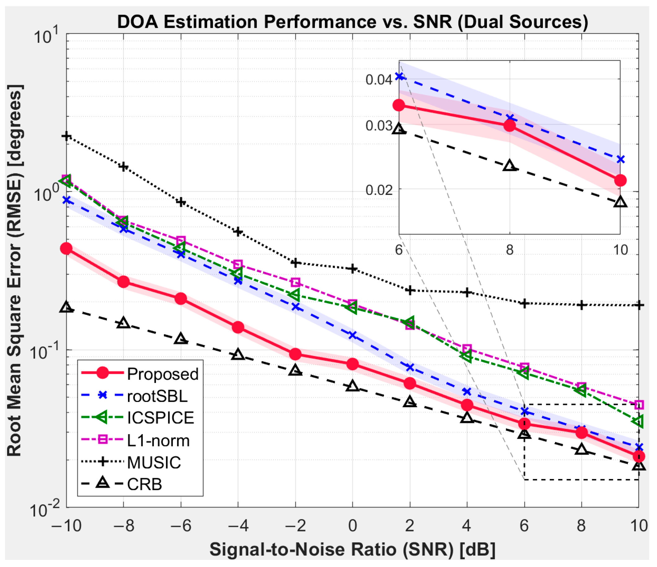
In the first experiment, we consider a scenario with K = 2 signal sources. The simulation parameters are detailed in the caption for Figure 2.

Figure 2 illustrates the RMSE performance of all compared methods as a function of the SNR. Several key observations can be made. First, our proposed algorithm consistently achieves the lowest RMSE across the entire SNR spectrum, demonstrating its superior accuracy. Second, in the challenging low-SNR region (e.g., from −10 dB to −4 dB), the performance gap between our method and the baselines is most pronounced. For instance, at an SNR of −8 dB, our algorithm’s RMSE is approximately ${0.6}^{°}$, whereas traditional methods like MUSIC and L1-norm exhibit errors exceeding ${1.5}^{°}$. This highlights the robustness of our Bayesian framework, where the sparse prior effectively suppresses noise-induced artifacts that degrade other methods.

Third, as the SNR increases, the performance of our algorithm rapidly approaches the theoretical Cramér–Rao bound (CRB). The zoomed-in inset for the high-SNR region (6 dB to 10 dB) clearly shows that the RMSE curve of our method (solid red line) nearly overlaps with the CRB (dashed black line). This indicates that our estimator is asymptotically efficient and unbiased. In contrast, other advanced sparse methods like rootSBL and ICSPICE, while performing well, maintain a discernible gap from the CRB, suggesting the presence of a performance floor due to their respective algorithmic or modeling limitations.

5.2.2. Performance with Three Signal Sources

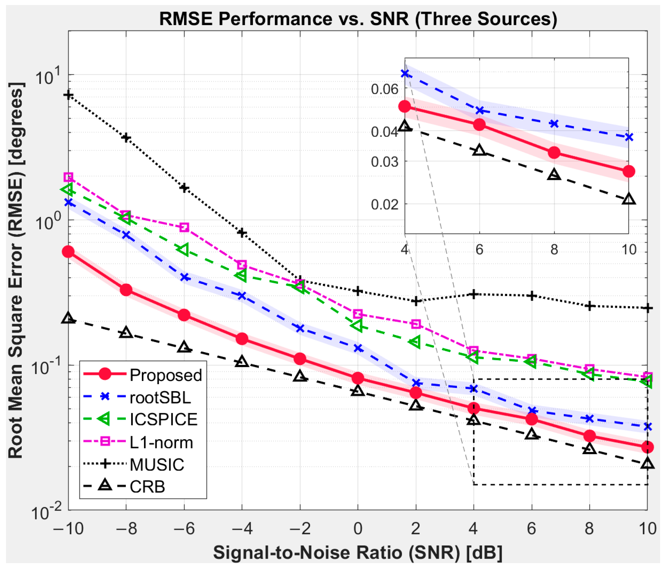
To assess the scalability of our algorithm, we increase the number of sources to K = 3. The specific setup is described in the caption for Figure 3.

As shown in Figure 3, the overall performance trends are consistent with the dual-source case, but the increased complexity of the scenario further accentuates the advantages of our proposed method. With more sources, the problem of signal aliasing becomes more severe, causing a general degradation in performance for all algorithms, especially at low SNRs.

However, our RC-FVSBL algorithm demonstrates remarkable resilience. At an SNR of −10 dB, its RMSE remains below $1^{°}$, while the errors for L1-norm and ICSPICE escalate to over $2^{°}$. This superior performance in a more crowded environment underscores the effectiveness of the FVSBL approach in accurately estimating the posterior distribution of the signal, even with increased parameter dimensionality. Furthermore, the inset in Figure 3 reaffirms that our method is the only one among the tested algorithms to achieve performance nearly identical to the CRB at high SNRs, solidifying its position as a highly accurate and robust DOA estimation technique. The ability to handle an increased number of sources gracefully is a critical requirement for practical applications in dense signal environments.

5.2.3. RMSE Versus Number of Snapshots

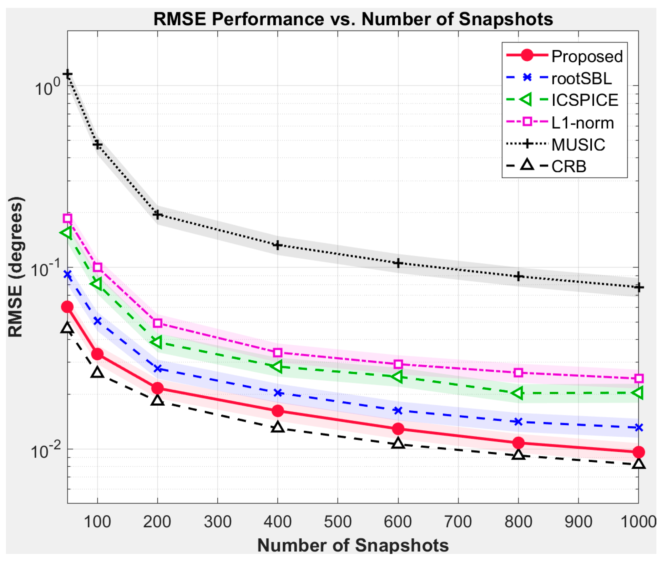
We now investigate the effect of the data record length on estimation accuracy by varying the number of available snapshots, L. The SNR is fixed at a moderately high value of 10 dB to isolate and emphasize the impact of the sample size on the performance of the algorithms. Other parameters are consistent with the dual-source scenario, as detailed in the caption for Figure 4.

As depicted in Figure 4, the RMSE for all algorithms improves as more snapshots become available. This is an expected trend, as a larger sample size leads to a more accurate and stable sample covariance matrix estimate, which is the foundation for all subsequent processing. However, the degree of improvement and the performance in sample-limited conditions vary significantly among the methods.

Our proposed RC-FVSBL demonstrates a pronounced advantage, particularly in the crucial sample-starved region (e.g., L < 200). At L = 50 snapshots, our method achieves an RMSE of approximately ${0.06}^{°}$. This is substantially lower than that of MUSIC (above ${1.0}^{°}$) and significantly better than other advanced sparse methods like rootSBL (approx. ${0.09}^{°}$) and ICSPICE (approx. ${0.15}^{°}$). This superior performance with very limited data is a critical advantage for practical applications in dynamic environments, such as tracking fast-moving targets, where the signal coherence time is short and only a few snapshots can be collected for each estimation.

Furthermore, as the number of snapshots increases, our algorithm’s performance curve smoothly converges toward the CRB. For L $\ge 600$, our method’s RMSE is nearly indistinguishable from the theoretical limit. In contrast, other methods like L1-norm and rootSBL exhibit a “flattening” effect at a level visibly above the CRB. This indicates that simply increasing the data volume cannot fully compensate for their inherent modeling biases or algorithmic limitations. This result strongly validates the asymptotic efficiency and robustness of our proposed estimator across different data record lengths.

5.3. Resolution and Convergence Analysis

Beyond standard RMSE performance, two other crucial metrics for practical DOA estimation systems are the ability to resolve closely spaced sources and the computational efficiency, which is often dictated by convergence speed. This section evaluates our algorithm’s performance in these two aspects.

5.3.1. Resolution Capability

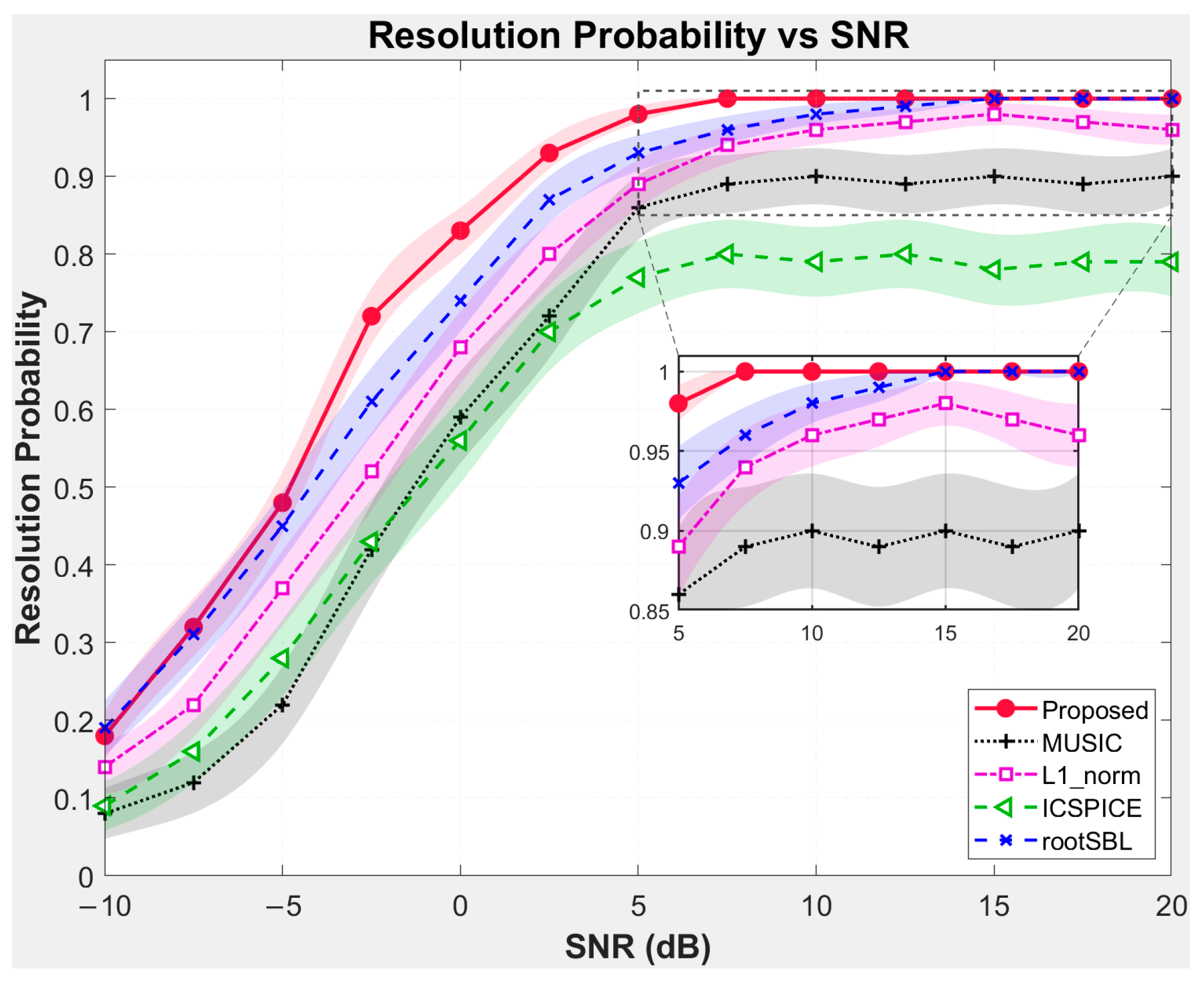
The ability to distinguish among signal sources arriving from very similar directions is a critical challenge in many sensing applications, such as traffic monitoring or target classification. We test this capability by placing two pairs of sources with small angular separations, as detailed in the caption for Figure 5.

The results are presented in Figure 5. The plot clearly demonstrates the superior resolution performance of our proposed RC-FVSBL algorithm. In the difficult low-to-moderate SNR range (−5 dB to 5 dB), our method consistently achieves a higher probability of successful resolution. For example, at an SNR of 0 dB, our algorithm successfully resolves the sources in over 80% of the trials, whereas L1-norm and ICSPICE achieve only around 65% and 55%, respectively. This enhanced resolution stems from the strong sparsity-inducing prior in the Bayesian framework, which favors solutions with a minimal number of active grid points, thereby producing a sharper spatial spectrum that is less prone to merging adjacent peaks.

As the SNR increases, all methods improve, but our algorithm is the first to reach near-perfect resolution. The inset shows that for an SNR $\ge$ 7.5 dB, our method achieves a resolution probability of 1.0, while other methods, including rootSBL, still exhibit occasional failures. This robust resolution capability makes our algorithm highly suitable for cluttered environments with closely spaced targets.

5.3.2. Convergence Speed

For real-time systems, the speed at which an algorithm converges to a final solution is as important as the accuracy of that solution. We evaluate the convergence behavior of the iterative algorithms in this experiment, with the results shown in Figure 6.

The convergence plot reveals a dramatic advantage for our proposed RC-FVSBL. Our algorithm achieves its final, low-RMSE solution in fewer than five iterations. The RMSE drops precipitously from the initial state to below ${0.1}^{°}$ and remains stable thereafter. In stark contrast, competing iterative methods, like rootSBL, L1-norm, and ICSPICE, exhibit much slower convergence. They require over 100 iterations to approach their final error values, and as the inset clearly shows, their final accuracy is still inferior to that of our method.

This remarkable acceleration is a direct consequence of the fast variational Bayesian learning (FVSBL) formulation introduced in Section 4.4. Traditional variational Bayesian methods rely on slow, cyclically dependent updates between parameters. Our FVSBL approach, however, transforms the hyperparameter update into a monotonic, closed-form root-finding problem. As proven in Appendix A, this ensures a direct and rapid trajectory toward the optimal solution, avoiding the oscillatory behavior and slow progress that plague other methods. This ultra-fast convergence is a key contributor to the overall computational efficiency of our algorithm, making it a highly attractive option for applications demanding low-latency processing.

5.4. Computational Complexity Analysis

To quantitatively validate the “accelerating” aspect of our proposed algorithm, this section analyzes its computational complexity from both a theoretical and an empirical standpoint. The efficiency of our method is a key contributor to its suitability for real-time applications.

5.4.1. Theoretical Complexity Analysis

The computational complexity of our proposed RC-FVSBL algorithm is primarily determined by the iterative updates of the posterior parameters and hyperparameters within the variational inference framework. Following the procedure outlined in Section 4, the main computational burden at each iteration can be broken down as follows:

• Posterior Covariance $\mathsf{\Sigma }$ Update: The most computationally intensive step is the calculation of the posterior covariance matrix, ${\mathsf{\Sigma }}^{(i+1)}={({\overline{\Psi }}^T\overline{\Psi }+\mathrm{diag}\{{\widehat{\gamma }}^{(i)}\})}^{-1}$. The matrix, $\overline{\Psi }$, has dimensions $R\times (N+1)$, where $R\le M^2$, and $\widehat{\gamma }$ is of size (N + 1). The matrix inversion of this $(N+1)\times (N+1)$ matrix dominates this step, requiring $O({(N+1)}^3)$, or simply $O(N^3)$ floating-point operations (FLOPs).
• Posterior Mean $\mu$ Update: The calculation of the posterior mean, ${\mu }^{(i+1)}={\mathsf{\Sigma }}^{(i+1)}{\overline{\Psi }}^T\overline{r}$, involves a matrix-vector product, which has a complexity of $O(N^2)$. This is computationally less demanding than the matrix inversion.
• Hyperparameter $\gamma$ Update (FVSBL Root-Finding): The FVSBL update for the hyperparameters, $\gamma$, involves solving N + 1 independent, single-variable root-finding problems (from Equation (A7)). Each root can be found efficiently using numerical methods like Newton’s method, which typically converges in a small, constant number of steps. Therefore, the total complexity for this update step is O (N).

Combining these steps, the total computational complexity per iteration of our proposed algorithm is dominated by the matrix inversion, resulting in a complexity of $O(N^3)+O(N^2)+O(N)\approx O(N^3)$.

We compare our algorithm with a representative SBL method, rootSBL. As summarized in

Table 2. Theoretical complexity comparison within the SBL framework.

Algorithm	Dominant Operation	Per-Iteration Complexity (FLOPs)
rootSBL	$\mathrm{Complex} \mathrm{matrix} \mathrm{inversion} (N\times N)$	$O(N^3)$
RC-FVSBL (proposed)	$\mathrm{Real}\text{-}\mathrm{valued} \mathrm{matrix} \mathrm{inversion} (N\times N)$	$O(N^3)$

, both algorithms share the same O ($N^3$) per-iteration complexity order.

However, our RC-FVSBL algorithm incorporates two crucial innovations that lead to a substantial reduction in the overall computational load, as follows:

• Acceleration via Real-Valued Transformation (Constant Factor Reduction): A key component of our method is the real-valued transformation applied to the sparse recovery problem. This transformation yields a substantial computational advantage that is not reflected in the order of complexity. While the $O(N^3)$ complexity of the matrix inversion remains, the nature of the underlying arithmetic is fundamentally changed. Standard complex matrix operations, which involve numerous complex multiplications (each comprising four real multiplications), are replaced by operations in the real domain. This substitution drastically reduces the number of floating-point operations required for each step of the matrix inversion, leading to a significant, constant-factor reduction in runtime.
• Acceleration via Fast Variational Bayesian Learning (FVSBL): The most significant source of acceleration stems from the FVSBL framework, which addresses the primary bottleneck of conventional SBL methods—the slow convergence rate. As demonstrated in our convergence analysis (Section 5.3.2), the FVSBL’s monotonic update scheme enables our algorithm to converge in a very small, constant number of iterations (typically fewer than ten). This contrasts sharply with traditional SBL implementations, such as rootSBL, which often require hundreds of iterations to reach a solution. Consequently, while the per-iteration complexity is $O(N^3)$, the total computational cost, which is the product of the per-iteration complexity and the number of iterations, is vastly lower for our method. This dramatic reduction in the required number of iterations is the principal driver of the overall acceleration.

5.4.2. Empirical Runtime Comparison Within the SBL Framework

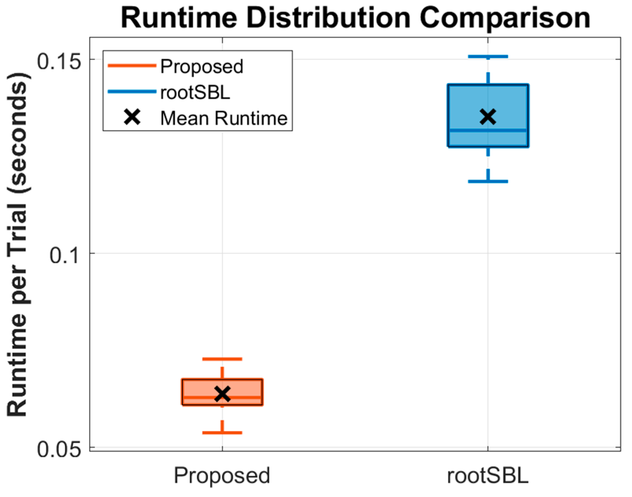
To empirically validate the acceleration achieved by our innovations, we provide a statistically robust comparison of the runtime performance. We measured the runtime distribution of our proposed RC-FVSBL and the baseline rootSBL over 100 independent Monte Carlo trials. The results are visualized using a box plot in Figure 7.

The plot reveals two key advantages of our proposed algorithm. First, in terms of central tendency, our algorithm is substantially faster. The mean runtime for our method is merely 0.0639 s, whereas rootSBL requires 0.1354 s on average. This represents a significant acceleration, with our algorithm being approximately 2.12 times faster than its state-of-the-art SBL competitor.

Second, and arguably as important for practical systems, our algorithm demonstrates significantly higher runtime stability. This is visually evident from the much more compact box and whisker plot for the “Proposed” method. The standard deviation of our algorithm’s runtime (0.0040 s) is less than half that of rootSBL (0.0085 s), indicating that its performance is highly consistent and predictable across different data realizations. This stability is a direct result of the FVSBL’s deterministic and rapid convergence path, which is less susceptible to variations in the input data compared to the slower, more uncertain convergence of traditional SBL methods.

In conclusion, the empirical data lend strong support to our theoretical analysis. The synergistic combination of the real-valued transformation and the FVSBL framework appears to be effective, as our method achieves a considerable speed-up over the conventional SBL approach while also exhibiting enhanced runtime stability.

5.5. Robustness Analysis Against Array Imperfections

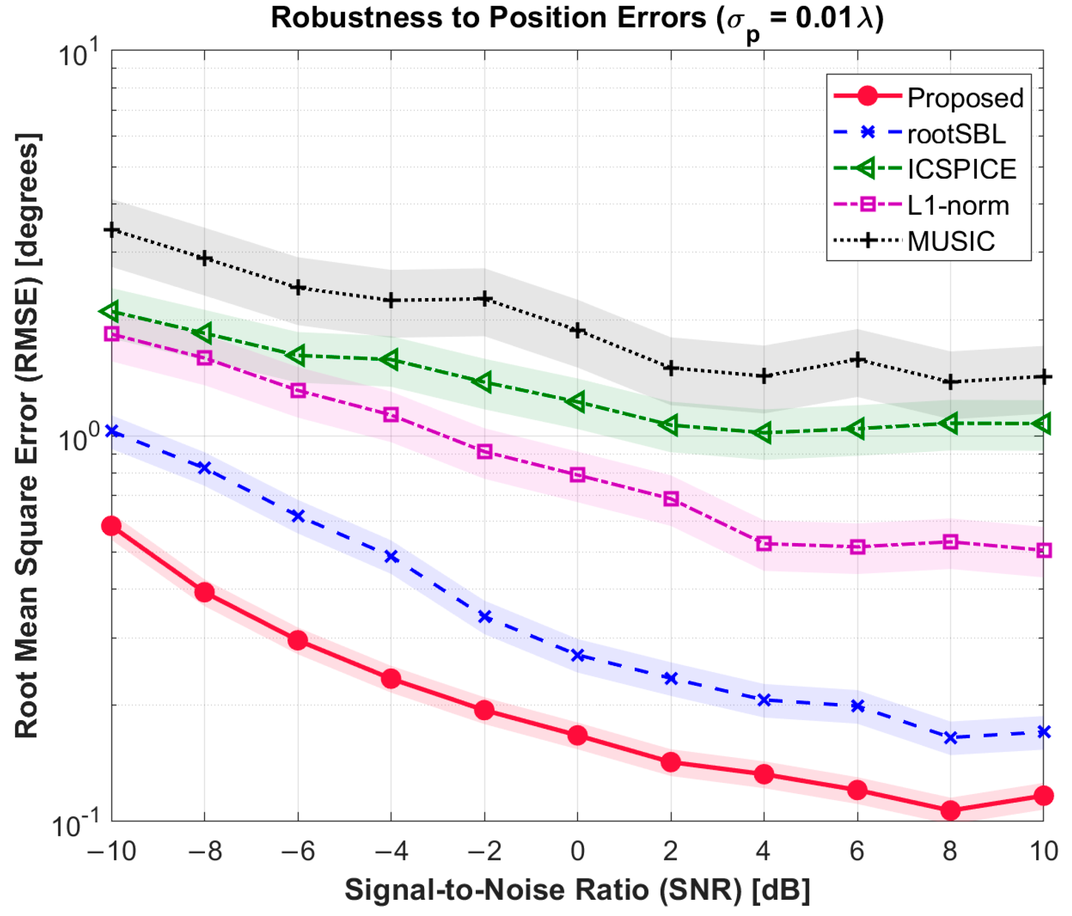
To evaluate the performance of our proposed algorithm under more practical, non-ideal conditions, we conducted a simulation to test its robustness against sensor position errors. This experiment serves as a proxy for real-world scenarios where the physical array geometry may deviate from its assumed model. We introduced a random, zero-mean Gaussian perturbation with a standard deviation of ${\sigma }_p=0.01\lambda$ to the position of each sensor in every Monte Carlo trial. All algorithms were then tasked with estimating the DOAs using the ideal, error-free array manifold, creating a controlled model mismatch scenario.

The results of this robustness test are presented in Figure 8. As expected, the presence of position errors leads to a performance degradation for all methods compared to the ideal case (Figure 2). However, the degree of this degradation varies significantly, clearly highlighting the differences in robustness.

Subspace-based methods, MUSIC and ICSPICE, prove to be the most sensitive to this model mismatch. Their RMSE curves are substantially elevated, indicating that their performance relies heavily on the precise knowledge of the array manifold, a condition that is compromised by the position errors.

In contrast, sparse recovery methods demonstrate superior resilience, with Bayesian approaches showing a particular advantage. Among them, our proposed RC-FVSBL consistently exhibits a higher level of robustness. Its performance curve remains the lowest across the majority of the SNR range. The performance gap between our method and rootSBL is most pronounced in the moderate SNR region (from 0 dB to 8 dB). For instance, at an SNR of 4 dB, the RMSE of our method is approximately ${0.12}^{°}$, while the RMSE of rootSBL is around ${0.25}^{°}$, which is more than twice as high.

This suggests that our algorithm’s structure, which combines a coherent processing front-end with a real-valued Bayesian framework, is more effective at mitigating the phase uncertainties introduced by sensor displacement. This superior robustness in the face of array imperfections is a critical feature, enhancing the viability and reliability of our algorithm for deployment in real-world sensing systems.

6. Conclusions

This paper presents a broadband OFDM signal direction-of-arrival (DOA) estimation method based on clustering focusing and fast variational sparse Bayesian learning (FVSBL). The method first utilizes an innovative frequency clustering technique to convert the broadband signal into an equivalent narrowband covariance matrix, effectively addressing the issue of inconsistent spatial information in broadband signals. It then employs real-valued transformation techniques to optimize the sparse equations, significantly reducing computational complexity. Finally, the improved FVSBL algorithm is used to achieve efficient and stable parameter estimation.

Our comprehensive simulation results have demonstrated the effectiveness of the proposed algorithm. Compared to several methods, RC-FVSBL shows superior performance in terms of estimation accuracy, particularly under challenging conditions such as low SNR, limited snapshots, and the presence of model imperfections like sensor position errors. Furthermore, the FVSBL framework was empirically shown to provide a substantial acceleration (over twofold) compared to conventional SBL approaches, making it a more viable candidate for time-sensitive applications.

Despite these promising results, we acknowledge certain limitations, which pave the way for future research. A key area for theoretical extension lies in the focusing stage. The current method’s reliance on preliminary DOA estimates can be a bottleneck in very-low-SNR scenarios. A more advanced direction, which we plan to pursue, is the development of a focusing-free or auto-focusing SBL framework. Such an approach would treat the focusing parameters as latent variables within a unified probabilistic model, allowing for their joint inference alongside the sparse signal. This would create a more robust and theoretically elegant end-to-end estimation system. Further theoretical work will also involve extending the framework’s applicability from ULAs to more complex array geometries, such as sparse or planar arrays.

Concurrently, we are developing a concrete plan for hardware-based validation to rigorously assess the algorithm’s real-world viability. Our planned experimental setup will utilize a multi-antenna software-defined radio (SDR) platform (e.g., USRP), configured as a ULA. We will transmit and receive 5G NR-compliant OFDM waveforms in a controlled indoor environment, starting with single-source and progressing to multi-source scenarios. This will allow us to evaluate the algorithm’s performance against real-world hardware impairments, including phase noise, I/Q imbalance, and antenna coupling, providing the ultimate validation of its practical utility.

In summary, this study contributes an effective and practical solution to the field of broadband signal DOA estimation. By addressing key limitations of existing methods, it holds significant potential for advancing applications in 5G sensing, radar, and wireless communications.

References

1. Qian, C.; Huang, L.; Sidiropoulos, N.D.; Xie, L. Enhanced PUMA for direction-of-arrival estimation and its performance analysis. IEEE Trans. Signal Process. 2016, 64, 4127–4137. [Google Scholar] [CrossRef]
2. Roy, R.; Kailath, T. ESPRIT-estimation of signal parameters via rotational invariance techniques. IEEE Trans. Acoust. Speech Signal Process. 1989, 37, 984–995. [Google Scholar] [CrossRef]
3. Schmidt, R. Multiple emitter location and signal parameter estimation. IEEE Trans. Antennas Propag. 1986, 34, 276–280. [Google Scholar] [CrossRef]
4. Shan, T.-J.; Wax, M.; Kailath, T. On spatial smoothing for direction-of-arrival estimation of coherent signals. IEEE Trans. Acoust. Speech Signal Process. 1985, 33, 806–811. [Google Scholar] [CrossRef]
5. Zhou, Z.; Jin, T.; Li, Y.; Zhang, M.; So, H.C. Enhanced Coherent DOA Estimation in Low SNR Environments Through Contrastive Learning. IEEE Trans. Instrum. Meas. 2025, 74, 1–21. [Google Scholar] [CrossRef]
6. Chen, T.; Kornblith, S.; Norouzi, M.; Hinton, G. A simple framework for contrastive learning of visual representations. In Proceedings of the 37th International Conference on Machine Learning, Vienna, Austria, 13–18 July 2020; pp. 1597–1607. [Google Scholar]
7. Deng, J.; Shi, W.; Zhang, J.; Ai, B. Supervised contrastive CSI representation learning for massive MIMO positioning. IEEE Commun. Lett. 2022, 26, 1799–1803. [Google Scholar] [CrossRef]
8. Gong, X.; Lu, A.-A.; Fu, X.; Zhang, H. Semisupervised Representation Contrastive Learning for Massive MIMO Fingerprint Positioning. IEEE Internet Things J. 2023, 11, 14870–14885. [Google Scholar] [CrossRef]
9. Li, Y.; Zhou, Z.; Chen, C.; Jin, T.; Zhang, M. An efficient convolutional neural network with supervised contrastive learning for multi-target DOA estimation in low SNR. Axioms 2023, 12, 862. [Google Scholar] [CrossRef]
10. Villani, M.J.; Schoots, N. Any deep relu network is shallow. arXiv 2023, arXiv:2306.11827. [Google Scholar] [CrossRef]
11. Cong, J.; Wang, X.; Huang, M.; Shan, T. Robust DOA estimation method for MIMO radar via deep neural networks. IEEE Sens. J. 2020, 21, 7498–7507. [Google Scholar] [CrossRef]
12. Cao, Y.; Lv, T.; Lin, Z.; Gao, H.; Yang, F. Complex ResNet aided DoA estimation for near-field MIMO systems. IEEE Trans. Veh. Technol. 2020, 69, 11139–11151. [Google Scholar] [CrossRef]
13. Wu, X.; Yang, X.; Jia, X.; Zhang, Y.; Zhang, Z. A gridless DOA estimation method based on convolutional neural network with Toeplitz prior. IEEE Signal Process. Lett. 2022, 29, 1247–1251. [Google Scholar] [CrossRef]
14. Lee, K. Deep learning-aided coherent direction-of-arrival estimation with the FTMR algorithm. IEEE Trans. Signal Process. 2022, 70, 1118–1130. [Google Scholar]
15. Papageorgiou, G.K.; Sellathurai, M.; Eldar, Y.C. Deep networks for direction-of-arrival estimation in low SNR. IEEE Trans. Signal Process. 2021, 69, 3714–3729. [Google Scholar] [CrossRef]
16. Zhu, Z.; Chen, C.; Yang, B. Angle of Arrival Estimation with Transformer: A Sparse and Gridless Method with Zero-Shot Capability. arXiv 2024, arXiv:2408.09362. [Google Scholar] [CrossRef]
17. Zheng, R.; Sun, S.; Liu, H.; Chen, H.; Li, J. Interpretable and efficient beamforming-based deep learning for single-snapshot DOA estimation. IEEE Sens. J. 2023, 24, 22096–22105. [Google Scholar] [CrossRef]
18. Stoica, P.; Babu, P.; Li, J. SPICE: A sparse covariance-based estimation method for array processing. IEEE Trans. Signal Process. 2010, 59, 629–638. [Google Scholar] [CrossRef]
19. Dai, J.; Xu, X.; Zhao, D. Direction-of-arrival estimation via real-valued sparse representation. IEEE Antennas Wirel. Propag. Lett. 2013, 12, 376–379. [Google Scholar] [CrossRef]
20. Hu, N.; Ye, Z.; Xu, X.; Tian, Y.; Lan, P. DOA estimation for sparse array via sparse signal reconstruction. IEEE Trans. Aerosp. Electron. Syst. 2013, 49, 760–773. [Google Scholar] [CrossRef]
21. Liu, Z.-M.; Huang, Z.-T.; Zhou, Y.-Y. Array signal processing via sparsity-inducing representation of the array covariance matrix. IEEE Trans. Aerosp. Electron. Syst. 2013, 49, 1710–1724. [Google Scholar] [CrossRef]
22. Liu, Z.-M.; Huang, Z.-T.; Zhou, Y.-Y.; Zheng, N. Direction-of-arrival estimation of noncircular signals via sparse representation. IEEE Trans. Aerosp. Electron. Syst. 2012, 48, 2690–2698. [Google Scholar] [CrossRef]
23. Malioutov, D.; Cetin, M.; Willsky, A.S. A sparse signal reconstruction perspective for source localization with sensor arrays. IEEE Trans. Signal Process. 2005, 53, 3010–3022. [Google Scholar] [CrossRef]
24. Zhang, L.; Dai, L. Image reconstruction of electrical capacitance tomography based on an efficient sparse Bayesian learning algorithm. IEEE Trans. Instrum. Meas. 2022, 71, 1–14. [Google Scholar] [CrossRef]
25. Pan, H.; Yang, Y.; Zheng, J.; Cheng, J.; Chen, X. Symplectic transformation based variational Bayesian learning and its applications to gear fault diagnosis. Measurement 2019, 147, 106827. [Google Scholar] [CrossRef]
26. Wang, Q.; Yu, H.; Li, J.; So, H.C.; Wan, Q. Sparse Bayesian learning using generalized double Pareto prior for DOA estimation. IEEE Signal Process. Lett. 2021, 28, 1744–1748. [Google Scholar] [CrossRef]
27. Dai, J.; So, H.C. Real-valued sparse Bayesian learning for DOA estimation with arbitrary linear arrays. IEEE Trans. Signal Process. 2021, 69, 4977–4990. [Google Scholar] [CrossRef]
28. Guo, Q.; Xin, Z.; Zhou, T.; Huang, T.; Yang, X. Off-grid space alternating sparse Bayesian learning. IEEE Trans. Instrum. Meas. 2023, 72, 1–10. [Google Scholar] [CrossRef]
29. Gerstoft, P.; Mecklenbräuker, C.F.; Xenaki, A.; Nannuru, S. Multisnapshot sparse Bayesian learning for DOA. IEEE Signal Process. Lett. 2016, 23, 1469–1473. [Google Scholar] [CrossRef]
30. Park, Y.; Meyer, F.; Gerstoft, P. Sequential sparse Bayesian learning for doa. In Proceedings of the 2020 54th Asilomar Conference on Signals, Systems, and Computers, Pacific Grove, CA, USA, 1–4 November 2020; pp. 78–81. [Google Scholar]
31. Ahmad, Z.; Song, Y.; Du, Q. Wideband DOA estimation based on incoherent signal subspace method. COMPEL-Int. J. Comput. Math. Electr. Electron. Eng. 2018, 37, 1271–1289. [Google Scholar] [CrossRef]
32. Valaee, S.; Kabal, P. Wideband array processing using a two-sided correlation transformation. IEEE Trans. Signal Process. 1995, 43, 160–172. [Google Scholar] [CrossRef]
33. Hung, H.; Kaveh, M. Focussing matrices for coherent signal-subspace processing. IEEE Trans. Acoust. Speech Signal Process. 1988, 36, 1272–1281. [Google Scholar] [CrossRef]
34. Doron, M.A.; Weiss, A.J. On focusing matrices for wide-band array processing. IEEE Trans. Signal Process. 1992, 40, 1295–1302. [Google Scholar] [CrossRef]
35. Swingler, D.N.; Krolik, J. Source location bias in the coherently focused high-resolution broad-band beamformer. IEEE Trans. Acoust. Speech Signal Process. 1989, 37, 143–145. [Google Scholar] [CrossRef]
36. Valaee, S.; Kabal, P. The optimal focusing subspace for coherent signal subspace processing. IEEE Trans. Signal Process. 1996, 44, 752–756. [Google Scholar] [CrossRef][Green Version]
37. Zhou, W.; Zhang, R.; Chen, G.; Wu, W. Integrated sensing and communication waveform design: A survey. IEEE Open J. Commun. Soc. 2022, 3, 1930–1949. [Google Scholar] [CrossRef]
38. Liu, R.; Li, M.; Liu, Q.; Swindlehurst, A.L. DOA estimation-oriented joint array partitioning and beamforming designs for ISAC systems. IEEE Trans. Wirel. Commun. 2024, 24, 2052–2066. [Google Scholar] [CrossRef]
39. Ottersten, B.; Stoica, P.; Roy, R. Covariance matching estimation techniques for array signal processing applications. Digit. Signal Process. 1998, 8, 185–210. [Google Scholar] [CrossRef]
40. Chen, F.; Dai, J.; Hu, N.; Wu, Z.; Xu, X. Sparse Bayesian learning for off-grid DOA estimation with nested arrays. Digit. Signal Process. 2018, 82, 187–193. [Google Scholar] [CrossRef]
41. Tzikas, D.G.; Likas, A.C.; Galatsanos, N.P. The variational approximation for Bayesian inference. IEEE Signal Process. Mag. 2008, 25, 131–146. [Google Scholar] [CrossRef]
42. Möderl, J.; Leitinger, E.; Fleury, B.H.; Pernkopf, F.; Witrisal, K. Fast variational block-sparse Bayesian learning. arXiv 2023, arXiv:2306.00442. [Google Scholar] [CrossRef]
Figure 1. Schematic of a Uniform Linear Array (ULA) for Direction-of-Arrival (DOA) estimation. The array consists of M sensors (circles) with inter-element spacing d. A far-field signal source (asterisk) impinges on the array from an angle θ relative to the array’s normal.
Electronics 14 03174 g001
Figure 2. Root mean square error (RMSE) performance versus signal-to-noise ratio (SNR) for two signal sources. The proposed algorithm is compared with MUSIC, L1-norm, ICSPICE, rootSBL, and the CRB. The true DOAs are located at [ 25.5 ° , 60.5 ° ] . The simulation is configured with a ULA of M = 20 sensors and L = 200 snapshots. The shaded areas represent the ± 1 standard deviation over 200 Monte Carlo trials. The inset provides a zoomed-in view of the high-SNR region to highlight performance differences.
Electronics 14 03174 g002
Figure 3. RMSE performance versus signal-to-noise ratio (SNR) for three signal sources. The true DOAs are located at [ 30.5 ° , 15.5 ° , 60.5 ° ] . Other simulation parameters, including M = 20, L = 200, and the number of Monte Carlo trials, are identical to those in Figure 2. The inset similarly provides a magnified view of the high-SNR performance.
Electronics 14 03174 g003
Figure 4. RMSE performance versus the number of snapshots (L). The experiment is conducted with two signal sources at [ 60.5 ° , 25.6 ° ] under a fixed SNR = 10 dB and an array size of M = 20. The number of snapshots varies from 50 to 1000. The shaded areas represent the ± 1 standard deviation over 200 Monte Carlo trials, illustrating the statistical consistency of the estimates.
Electronics 14 03174 g004
Figure 5. Resolution probability versus SNR for two pairs of closely spaced sources. The four sources are located at [ 32.5 ° , 30.5 ° ] , [ 30.5 ° , 32.5 ° ] , with each pair separated by only 2.0 ° . A successful resolution is registered if four distinct DOAs are found with an estimation error of less than 1.0 ° for each. The simulation uses M = 20 and L = 200. The shaded areas indicate the ± 1 standard deviation over 200 Monte Carlo trials.
Electronics 14 03174 g005
Figure 6. Convergence performance of the iterative algorithms. The plot shows the RMSE as a function of the iteration number for a dual-source scenario ( [ 60.3 ° , 25.6 ° ] ) at a challenging SNR = 0 dB. The non-iterative MUSIC algorithm is plotted as a horizontal line for reference. The inset provides a magnified view of the final convergence state. M = 20 and L = 200.
Electronics 14 03174 g006
Figure 7. Runtime distribution comparison between the proposed RC-FVSBL and rootSBL. The box plot displays the distribution of the wall-clock time per trial, collected over 100 independent Monte Carlo runs. The simulation scenario is identical to that in Section 5.2.1 (M = 20, L = 200, and SNR = 0 dB). The central line in each box indicates the median, the box edges represent the 25th and 75th percentiles, the whiskers extend to the most extreme data points within 1.5 times the interquartile range, and the “x” marker denotes the mean runtime.
Electronics 14 03174 g007
Figure 8. Robustness to sensor position errors. This plot shows the RMSE performance versus the SNR when the position of each sensor is subject to a random Gaussian perturbation with a standard deviation of σ p = 0.01 λ . All algorithms operate using the ideal, unperturbed array manifold, thus testing their resilience to model mismatch. The shaded areas represent the ± 1 standard deviation over 200 Monte Carlo trials.
Electronics 14 03174 g008