Article

Feedback Linearization for a Generalized Multivariable T-S Model

by
Basil Mohammed Al-Hadithi
1,2,*,
Javier Blanco Rico
3 and
Agustín Jiménez
1
1
Intelligent Control Group, Centre for Automation and Robotics UPM—CSIC, Universidad Politécnica de Madrid, 28006 Madrid, Spain
2
Department of Electrical, Electronics, Control Engineering and Applied Physics, School of Industrial Design and Engineering, Universidad Politécnica de Madrid, 28012 Madrid, Spain
3
Escuela Técnica Superior de Ingenieros Industriales, Universidad Politécnica de Madrid, 28006 Madrid, Spain
*
Author to whom correspondence should be addressed.
Electronics 2025, 14(15), 3129; https://doi.org/10.3390/electronics14153129
Submission received: 9 June 2025 / Revised: 19 July 2025 / Accepted: 4 August 2025 / Published: 6 August 2025
(This article belongs to the Section Systems & Control Engineering)

Abstract

This study presents a novel optimal fuzzy logic control (FLC) strategy based on feedback linearization for the regulation of multivariable nonlinear systems. Building upon an enhanced Takagi–Sugeno (T-S) model previously developed by the authors, the proposed method incorporates a refined parameter-weighting scheme to optimize both local and global approximations within the T-S framework. This approach enables improved selection and minimization of the performance index. The effectiveness of the control strategy is validated through its application to a two-link serial robotic manipulator. The results demonstrate that the proposed FLC achieves robust performance, maintaining system stability and high accuracy even under the influence of noise and load disturbances, with well-damped system behavior and negligible steady-state error.

1. Introduction

Controlling complex systems remains one of the most significant challenges and achievements in modern control theory. Particularly, nonlinear systems, multiple-input multiple-output (MIMO) systems, and systems with significant uncertainties are common in real-world applications yet notoriously difficult to control using conventional techniques. To address these challenges, ongoing research continues to explore and refine analysis tools and control strategies that offer systematic solutions for such complex problems.
This paper introduces a novel controller designed to manage systems exhibiting all three of these challenging characteristics: nonlinearity, multiple variables, and uncertainty. The proposed approach integrates feedback linearization with fuzzy modeling, offering a robust and optimal control solution capable of handling a wide range of operational conditions.
Feedback linearization has emerged as a powerful nonlinear control strategy, gaining widespread adoption over the past few decades. Its key advantage lies in transforming a nonlinear open-loop system into a linearized closed-loop system, typically with a broader effective operating region compared to classical Jacobian-based linearization around an equilibrium point [1]. This method has demonstrated success across diverse domains: from classic pendulum systems [2] and power electronics [3] to highly nonlinear and uncertain platforms such as space payloads [4] and robotic manipulators [5].
Though not universally applicable, feedback linearization provides a flexible framework that accommodates advanced control techniques, including sliding mode control (SMC) [6], and supports integration with learning-based methods, such as neural network-enhanced linearization for systems with dynamic uncertainties [7].
However, even the most sophisticated control strategies rely heavily on accurate system modeling. In this context, fuzzy logic has proven especially effective for modeling complex, nonlinear systems. By encoding expert knowledge or empirical data into rule-based representations, fuzzy modeling enables the derivation of structured system models suitable for control design [8].
Among the various fuzzy modeling approaches, Takagi–Sugeno (T-S) models [9] have become particularly prominent (e.g., see [10,11,12,13]). These models offer powerful approximation capabilities and support rigorous stability analysis and control design, even for MIMO systems [14,15,16]. Their architecture, based on locally affine models blended through fuzzy membership functions (MFs), facilitates the use of data-driven identification techniques, enhancing their adaptability to real-world systems.
Recent research has continued to enhance the accuracy and computational efficiency of T-S models. Techniques aimed at reducing identification complexity, improving convergence speed, and ensuring robustness have been explored in multiple studies [17,18]. Other contributions have focused on theoretical aspects, such as the pros and cons of different kinds of models [19]; stability guarantees; and convergence criteria for fuzzy systems [20,21]. These developments help extend the applicability of T-S models to higher-order systems with more inputs and outputs [22].
A particularly relevant application domain is that of robotic systems, which are classic examples of nonlinear systems with parameter uncertainties and time-varying external disturbances. T-S fuzzy models have proven highly suitable for modeling and controlling these systems [23,24]. Their robustness under challenging operating conditions, such as sudden load changes or sensor noise, has been demonstrated in a variety of practical studies [25,26].
Furthermore, fuzzy FLC is particularly advantageous for enabling interaction with the robot’s environment, especially in unstructured settings where the nature of obstacles is dynamic and often unknown. Notable applications include goods transportation in storage facilities [27], as well as scenarios involving physical interaction with the environment, such as during collisions or when connecting to infrastructure [28].
This article contributes to an ongoing line of research by the authors, building on prior work ([29,30,31]) that proposed improved methodologies for estimating local and global T-S models. In particular, these efforts addressed limitations of traditional identification methods, such as restrictions on non-overlapping membership functions, through a novel weighting parameter approach that reduces the computational cost without sacrificing accuracy.
The current study extends these contributions by enhancing the Fuzzy Logic Controller with Linear Quadratic Regulator (FLC-LQR) architecture introduced in [29]. The new controller includes a time-based control action for trajectory convergence and introduces mechanisms to maintain performance even in the presence of modeling errors and external disturbances.
The integration of Fuzzy Logic Controllers (FLCs) with feedback linearization techniques has also gained attention in recent studies. Several studies have proposed hybrid methods to leverage the strengths of both paradigms (e.g., [32,33,34]). For instance, in [35] the authors present a fuzzy feedback linearization control for nonlinear T-S systems. The main difference from the proposed work is that in [35], the designed algorithm was applied to a single-input–single-output system, while in this work, the proposed controller is applied to multivariable systems. Another difference is that the robustness of the proposed controller is shown by subjecting it to disturbance and noise effects.
The main contributions of this paper are as follows:
  • The development of an optimal feedback linearization-based FLC, grounded in the authors’ improved T-S modeling framework and integrated with Linear Quadratic Regulator (LQR) optimal control.
  • Validation of the proposed controller through implementation on a two-link robotic manipulator, demonstrating robust performance, zero steady-state error, and effective disturbance rejection.
The structure of this paper is as follows: Section 2 reviews the fundamentals of feedback linearization. Section 3 introduces a control algorithm, ensuring zero steady-state error. Section 4 details the proposed optimal FLC-LQR methodology. Section 5 discusses fuzzy model identification and estimation, including the use of parameter weighting and constraints of the T-S framework. Section 6 outlines the implementation procedure. Section 7 presents the experimental validation on a two-link robot and compares the proposed method with conventional T-S-based approaches. Section 8 concludes the paper with final remarks and perspectives for future work.

2. Feedback Linearization

Feedback linearization is a widely adopted methodology in nonlinear control system design that has seen significant development over the past few decades. Its core principle lies in transforming a nonlinear system, either partially or fully, into a linear one through a carefully designed feedback mechanism. Unlike conventional Jacobian linearization, which locally approximates nonlinear behavior around an equilibrium point, feedback linearization achieves global or semi-global linearization by explicitly canceling out nonlinear dynamics through state and input transformations. This process enables the direct application of linear control techniques to the resulting linearized closed-loop system.
In this section, we introduce the foundational concepts and formal procedures involved in feedback linearization. In the following section, this methodology will be further extended to include an integral action, aiming to eliminate steady-state errors in the controlled system. However, it is worth noting that practical implementations of feedback linearization often require supplementary mechanisms (such as anti-windup strategies and signal filtering) to account for real-world issues not captured by the theoretical model, including actuator saturation and measurement noise.
We start by modeling the system to be controlled as an affine system in its canonical form. It is modeled as follows:
x ˙ ( t ) = A 0 ( x ( t ) ) + A ( x ( t ) ) x ( t ) + B ( x ( t ) ) u ( t ) y ( t ) = C x ( t )
where x ˙ ( t ) denotes the time derivative of the state vector x ( t ) ; u ( t ) is the system input; y ( t ) is the output; A 0 ( x ( t ) ) represents the drift dynamics or the nonlinear bias term; A ( x ( t ) ) and B ( x ( t ) ) are state-dependant matrices defining the linear and input coupling terms, respectively; and C is the output matrix, assumed to be constant in this formulation. The second equation dictates the output of the system, which in this particular model is only dependent on the state vector based on the relation matrix C. The dimensions of the variables and functions involved are specified as
x : n y : q u : m A 0 : n n A : n n × n B : n n × m C : q × n
We assume that the system satisfies the condition n m , ensuring that the number of state variables is at least as large as the number of inputs. This forms the basis upon which the feedback linearization procedure is constructed in the subsequent sections.
The canonical form of the system’s matrices has the following structure:
A 0 = A 01 A 02 A 0 m , A 0 i = 0 0 a 0 i n i
A = A 11 A 12 A 1 m A 21 A 22 A 2 m A m 1 A m 2 A m m
A i i = 0 1 0 0 0 0 1 0 0 0 0 1 a i i 1 a i i 2 a i i 3 a i i n i n i × n i
A i j = 0 0 0 0 0 0 0 0 0 0 0 0 a i j 1 a i j 2 a i j 3 a i j n j n i × n j
B = B 1 B 2 B m , B i = 0 0 0 0 0 0 b i 1 b i 2 b i m n i × m
where n 1 , n 2 , , n m denote the dimensions of the controllable subspaces associated with each input.
Our primary objective is to reach the desired final zero state, regardless of the initial state. To this end, we define the following matrix:
S = S 11 S 12 S 1 m S 21 S 22 S 2 m S m 1 S m 2 S m m m × n
S i i = 0 0 0 1 n i 1 × n i
S i j = 0 0 0 0 1 × n j
If the feedback system is required to have a system matrix A f with the same structure as A ( x ( t ) ) , then the control action must be
u ( t ) = [ S B ( x ( t ) ] 1 S [ A 0 ( x ( t ) ) + ( A ( x ( t ) ) A f ) x ( t ) ]
assuming that the matrix S B ( x ( t ) ) is non-singular throughout the entire operational workspace. Under this assumption, the feedback system becomes
x ˙ ( t ) = A 0 ( x ( t ) ) + A ( x ( t ) ) x ( t ) B ( x ( t ) ) [ S B ( x ( t ) ) ] 1 S [ A 0 ( x ( t ) ) + ( A ( x ( t ) ) A f ) x ( t ) ]
Note that
S B = b 11 b 12 b 1 m b 21 b 22 b 2 m b m 1 b m 2 b m m m × m
and therefore,
B [ S B ] 1 = B 1 * B 2 * B m * n × m
B i * = B i [ S B ] 1 = 0 0 0 0 0 0 b i 1 b i 2 b i m b 11 b 12 b 1 m b 21 b 22 b 2 m b m 1 b m 2 b m m 1   = 0 0 0 0 0 0 0 0 0 1 n i i 0 0
This means that
B [ S B ] 1 = S T
fulfilling
B [ S B ] 1 S = S T S n × n
S T S = S ˜ 11 S ˜ 12 S ˜ 1 m S ˜ 21 S ˜ 22 S ˜ 2 m S ˜ m 1 S ˜ m 2 S ˜ m m
S ˜ i i = 0 0 0 0 0 0 0 0 1 n i n i n i × n i , S i j = 0 n i × n j
Therefore, it will satisfy the following:
B [ S B ] 1 S A 0 = A 0
A B [ S B ] 1 S [ A A f ] = A f
Consequently, the system adopts the following structure:
x ˙ ( t ) = A f x ( t )

3. Steady State Error

We now turn our attention to the problem of ensuring that, at the steady state, the system output variables y p reach their set points. A conventional approach to achieve zero steady-state error is to incorporate integral action, which is equivalent to introducing a set of q additional states defined as follows:
w ˙ ( t ) = y p y ( t ) = y p C x ( t ) w : q
We define the following extended state vector:
x e ( t ) = w ( t ) x ( t )
Consequently, w ( t ) represents the integral of the position error, and the complete system is given by
x ˙ e ( t ) = 0 A 0 ( x ( t ) ) + 0 C 0 A ( x ( t ) ) x e ( t ) + 0 B ( x ( t ) ) u ( t ) + I 0 y p y ( t ) = 0 C x e ( t )
For this augmented system, the following control action is proposed:
u ( t ) = [ S B ( x ( t ) ] 1 S [ A 0 ( x ( t ) ) + ( A ( x ( t ) ) A f ) x ( t ) K w ( t ) ]
where
K = K 1 K 2 K m , K i = 0 0 0 0 0 0 K i 1 K i 2 K i q R n i × q
It can be verified that
x ˙ ( t ) = A 0 ( x ( t ) ) + A ( x ( t ) ) x ( t ) B ( x ( t ) ) [ S B ( x ( t ) ) ] 1 S [ A 0 ( x ( t ) ) + ( A ( x ( t ) ) A f ) x ( t ) ]   + B ( x ( t ) ) [ S B ( x ( t ) ) ] 1 S K w ( t ) x ˙ ( t ) = A f x ( t ) + K w ( t )
and therefore, the feedback system takes the following form:
x ˙ e ( t ) = 0 C K A f x e ( t ) + I 0 y p y ( t ) = 0 C x e ( t )
The dynamics of this system are governed by the new system matrix, and if it stable, the system will reach a steady state:
x s = lim t x e ( t ) = w s x s x e = 0 y s = C x s
It can be verified that
0 0 = 0 C K A f w s x s + I 0 y p 0 = C x s + y p y s = 0 C x e ( t ) y s = C x s = y p
This implies that the control objective of achieving zero steady-state error has been met.

4. Optimal Controller Design

To select the appropriate control matrices A f and K, this work proposes designing these matrices based on a representative central operating point of the system:
x ˙ ( t ) = A c x ( t ) + B c u ( t ) y ( t ) = C x ( t )
Therefore, the extended system incorporating integral action is given by
x ˙ e ( t ) = 0 C 0 A c x ˙ e ( t ) + 0 B c u ( t ) + I 0 y p y ( t ) = 0 C x ˙ e ( t )
Assuming that y p = 0 , it follows that
x ˙ e ( t ) = 0 C 0 A c x ˙ e ( t ) + 0 B c u ( t )
We now seek the control action u ( t ) that drives the state from an arbitrary initial condition x e ( t 0 ) to the desired final zero state. To achieve this, we employ an LQR to minimize the quadratic performance criterion:
J = t 0 ( x e t ( t ) Q x e ( t ) + u t R u ) d t
where Q ( n + q ) × ( n + q ) and R m × m are symmetric positive definite matrices. The optimal control law is determined by the following equation:
u ( t ) = K w K x x e ( t )
K w K x = R 1 B c t L
where L n × n is the solution to the following Riccati equation:
0 = Q + L B c R 1 B c t L L A c A c t L
Thus, the closed-loop systems will behave as
x ˙ e ( t ) = 0 C 0 A c x e ( t ) + 0 B c u ( t )   = 0 C K A c x e ( t ) 0 B c K w K x x e ( t )
x ˙ e ( t ) = 0 C B c K w A c B c K x x e ( t )
Therefore, the goal is for the feedback linearized system to emulate the optimal system described in (20). In other words, the desired feedback system matrix is proposed as
K = B c K w
A f = A c B c K x
where K is the feedback matrix associated with the integral position error w ( t ) and A f is the desired feedback system matrix.
This approach ensures optimal dynamics at a representative central operating point.

5. Fuzzy T-S Model Parameter Estimation

To obtain the system matrices given in (1), we propose using the T-S identification method [9], which estimates system parameters by minimizing a performance index. An enhancement to the traditional T-S modeling approach is presented by the authors in [29].
The proposed method employs functions such as the following for identification:
f : n
y = f ( x 1 , x 1 , , x n )
These functions can be transformed into if–then rules for an n t h -order system:
S ( i 1 i m ) : I f z 1 i s M 1 i 1 a n d   z m i s M m i m t h e n y ^ = p 0 ( i 1 i m ) + p 1 ( i 1 i m ) x 1 + + p n ( i 1 i m ) x n
where y ,   x 1 ,   x 2 ,   ,   x n are measurable variables, and z 1 ,   z 2 ,   ,   z m is a subset of x 1 ,   x 2 ,   ,   x n .
The fuzzy estimation of the output is given by
y ^ = i 1 = 1 r 1 i m = 1 r m β ( i 1 i m ) ( z ) p 0 ( i 1 i m ) + p 1 ( i 1 i m ) x 1 + + p n ( i 1 i m ) x n
where
β k ( i 1 i m ) ( z ) = μ 1 i 1 ( z 1 ) μ 2 i 2 ( z 2 ) μ m i m ( z m ) j 1 = 1 r 1 j m = 1 r m μ 1 j 1 ( z 1 ) μ 2 j 2 ( z 2 ) μ m j m ( z m )
and μ j i j ( z j ) denotes the membership function corresponding to the set M j i j .
Fuzzy system parameters can be obtained by minimizing the following quadratic performance index, where the series x 1 k , x 2 k , , x n k , y k represents a set of N input/output samples:
J = k = 1 N ( y k y ^ k ) 2 = Y X P 2
with
Y = y 1 y 2 y N T P = p 0 ( 1 1 ) p 1 ( 1 1 ) p 2 ( 1 1 ) p n ( 1 1 ) p 0 ( r 1 r m ) p n ( r 1 r m ) T X = β 1 ( 1 1 ) β 1 ( 1 1 ) x 11 β 1 ( 1 1 ) x n 1 β 1 ( r 1 r m ) β 1 ( r 1 r m ) x n 1 β N ( 1 1 ) β N ( 1 1 ) x 1 N β N ( 1 1 ) x n N β N ( r 1 r N ) β N ( r 1 r m ) x n N
If X is a full-rank matrix, a solution can be obtained directly as
J = Y X P 2 = ( Y X P ) T ( Y X P ) J = X T ( Y X P ) = X T Y X T X P = 0 P = ( X T X ) 1 X T Y
A limitation of the methodology presented in [9] is that it cannot be applied to the most common type of MFs, such as those illustrated in Figure 1.
The membership functions
μ i 1 ( v i ) = b i v i b i a i and μ i 2 ( v i ) = v i a i b i a i
are defined over the interval [ a i , b i ] , which must satisfy the following condition:
μ i 1 ( a i ) = 1 μ i 1 ( b i ) = 0 μ i 2 ( a i ) = 0 μ i 2 ( b i ) = 1 μ i 1 ( v i ) + μ i 2 ( v i ) = 1
It has been demonstrated [29,30,31] that, in this common case, the matrix X is rank-deficient. Consequently, X T X is not invertible, preventing the direct application of the aforementioned method. A detailed proof can be found in [31].
When the matrix X is not of full rank, an efficient approach with low computational complexity, based on the well-known parameter-weighting method, is presented in [31].
Another advantage of this method is its capability to tune the T-S model parameters using experimental data. To achieve this, we begin with an initial parameter estimation as follows:
p 0 = [ p 0 0 p 1 0 p 2 0 p n 0 ] T
which may be obtained, for example, through a preliminary least squares analysis of the system under known operating conditions. This initial estimate serves as a reference in the calculation of the final system parameters. The fuzzy model parameters are then determined by minimizing the following function:
J = k = 1 N ( y k y ^ k ) 2 + γ 2 i 1 = 1 r 1 i m = 1 r m j = 0 m ( p j 0 p j ( i 1 i m ) ) 2   = Y X P 2 + γ 2 P 0 P 2   = Y γ P 0 X γ I P 2   = Y a X a P 2
where
P 0 = [ p 0 p 0 p 0 ] T r 1 . r 2 r m
where γ is a parameter representing the confidence level of the initial estimation [29,31].
When applied to a multivariable system, it is composed of a vector-valued function of the following form:
f : n q
y = f ( x 1 , x 2 , , x n ) y q
or, equivalently, as a set of q scalar functions
y j = f j ( x 1 , x 2 , , x n ) y , j = 1 q
For each of these functions, a MF can be modeled as
S j ( i 1 i m ) : I f z 1 i s M j 1 i 1 a n d z 2 i s M j 2 i 2 a n d z m i s M j m i m t h e n y ^ j = p j 0 ( i 1 i m ) + p j 1 ( i 1 i m ) x 1 + p j 2 ( i 1 i m ) x 2 + + p j n ( i 1 i m ) x n
When applied to the entire model, the basic system takes the following form:
Y N = y j 1 y j 2 y j N T P j = p j 0 ( 1 1 ) p j 1 ( 1 1 ) p j 2 ( 1 1 ) p j n ( 1 1 ) p j 0 ( r 1 r m ) p j n ( r 1 r m ) T X j = β j 1 ( 1 1 ) β j 1 ( 1 1 ) x 11 β j 1 ( 1 1 ) x n 1 β j 1 ( r 1 r m ) β j 1 ( r 1 r m ) x n 1 β j N 1 1 β j N ( 1 1 ) x 1 N β j N ( 1 1 ) x n N β j N ( r 1 r m ) β j N ( r 1 r m ) x n N
accompanied by the tuning equation:
J j = Y j Γ j P j 0 X j Γ j P j 2
Furthermore, it is common for all premises of the system to be identical, implying that in such cases,
X 1 = X 2 = = X q = X
If, in addition, the weighting factors γ j ( i 1 i m ) for all parameters of Γ are equal, then
J = Y 1 Y 2 Y q Γ P 10 Γ P 20 Γ P q 0 X Γ P 1 P 2 P m 2
J = Y a X a P 2
with the solution remaining as
P = ( X a t X a ) 1 X a t Y a
A detailed proof is provided in [29].

6. Implementation of the Proposed Method

The proposed control method is summarized in the following steps, which are organized into offline and online tasks.
Offline tasks:
  • Obtain the T-S model through experimentation: A 0 ( x ( t ) ) , A ( x ( t ) ) , B ( x ( t ) ) , and C.
  • Determine a central working point for the system; this may correspond to the central rule of the T-S model or the p 0 parameters from Section 5: A c and B c .
  • Compute the desired system matrix and the steady-state error cancellation matrix using LQR: A f and K.
  • Determine the matrix S.
Online tasks:
  • Update the system matrices at the current instant: A 0 ( x ( t ) ) , A ( x ( t ) ) , and B ( x ( t ) ) at the current time.
  • Update the control action u ( t ) at the current time using Equation (7).

7. Example: Two-Link Robot

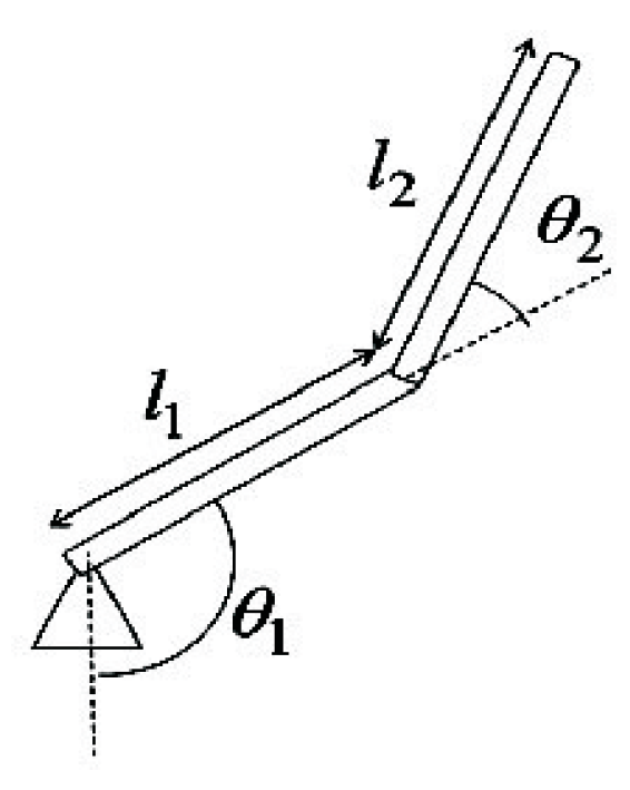
To illustrate the application of the proposed control methodology, consider a simple two-link robot, as shown in Figure 2. Each articulated joint is driven by a motor equipped with an encoder and a tachometer, providing torque as well as measurements of position and velocity. The system input consists of desired joint positions θ 1 and θ 2 or joint position trajectories θ d 1 ( t ) and θ d 2 ( t ) , which are specified by the robot’s control unit. These conditions are typical in industrial robots tasked with following prescribed paths.
The Lagrangian dynamical model of this type of robot is given by
H 11 H 12 H 21 H 22 θ ¨ 1 θ ¨ 2 + h θ ˙ 2 + β 1 h θ ˙ 1 h θ ˙ 2 h θ ˙ 1 β 2 θ ˙ 1 θ ˙ 2 + g 1 g 2 = τ 1 τ 2
where θ = [ θ 1 θ 2 ] T denotes the joint angles in radians, and τ = [ τ 1 τ 2 ] T represents the input torque at each joint in Newton-meters. The terms H i j correspond to the elements of the inertia matrix, defined as
H 11 = m 1 l c 1 2 + I 1 + m 2 ( l 1 2 + l c 2 2 + 2 l 1 l c 2 c o s θ 2 ) + I 2 H 12 = m 2 l 1 l c 2 c o s θ 2 + m 2 l c 2 2 + I 2 H 21 = H 12 H 22 = m 2 l c 2 2 + I 2
Here, m i is the mass of the i t h link in kilograms; l c i is the distance from the ( i 1 ) t h joint to the center of mass of the i t h link (whose total length is l i ), measured in meters; and I i denotes the moment of inertia of the i t h link, expressed in kilogram–meter squared. The term h is defined as
h = m 2 l 1 l c 2 s i n θ 2
The viscous friction coefficients β 1 and β 2 , given in kilogram–meter squared per second, form part of the centripetal and Coriolis force matrix. Finally, g 1 and g 2 represent the gravity compensation terms for each link, with g = 9.81 m/s2 denoting the gravitational acceleration, where
g 1 = m 1 l c 1 g s i n θ 1 + m 2 g ( l c 2 s i n ( θ 1 + θ 2 ) + l 1 s i n θ 1 ) g 2 = m 2 l c 2 g s i n ( θ 1 + θ 2 )
In our specific example, we consider a robot with the following characteristics:
m 1 = 2 kg , l 1 = 1 m , l c 1 = 0.5 m , I 1 = 0.25 kg m 2 , β 1 = 0.05 kg m 2 s
m 2 = 1.5 kg , l 2 = 1 m , l c 2 = 0.75 m , I 2 = 0.12 kg m 2 , β 2 = 0.05 kg m 2 s
For
θ 1 = θ ˙ 1 = θ 2 = θ ˙ 2 = 0
it can be verified that
τ 10 = g 10 = 0 , τ 20 = g 20 = 0

7.1. T-S Model

The states of the model are defined as
x = θ 1 θ ˙ 1 θ 2 θ ˙ 2 T
In this nonlinear system, the input torque pair [ τ 1 , τ 2 ] is linearly dependent, implying that the T-S rules do not depend on the control inputs. Suppose we assign three fuzzy sets to each state variable; given that there are four state variables, the complete rule base will consist of 3 4 = 81 rules of the following form:
S ( i 1 i n ) : If x 1 is M 1 i 1 and x 4 is M 4 i 4 then x ˙ = 0 a 20 ( i 1 i 2 i 3 i 4 ) 0 a 40 ( i 1 i 2 i 3 i 4 ) + 0 1 0 0 a 21 ( i 1 i 2 i 3 i 4 ) a 22 ( i 1 i 2 i 3 i 4 ) a 23 ( i 1 i 2 i 3 i 4 ) a 24 ( i 1 i 2 i 3 i 4 ) 0 0 0 1 a 41 ( i 1 i 2 i 3 i 4 ) a 42 ( i 1 i 2 i 3 i 4 ) a 43 ( i 1 i 2 i 3 i 4 ) a 44 ( i 1 i 2 i 3 i 4 ) x + 0 0 b 21 ( i 1 i 2 i 3 i 4 ) b 22 ( i 1 i 2 i 3 i 4 ) 0 0 b 41 ( i 1 i 2 i 3 i 4 ) b 42 ( i 1 i 2 i 3 i 4 ) τ 1 τ 2
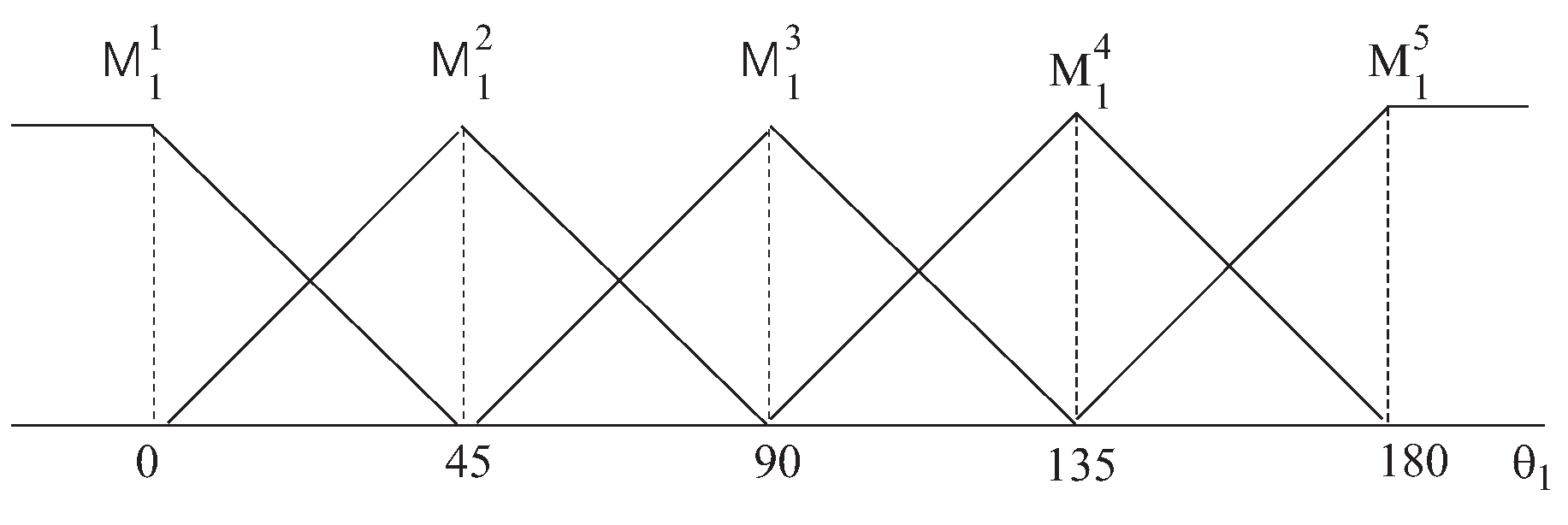
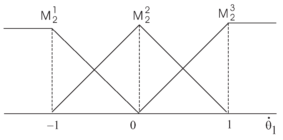
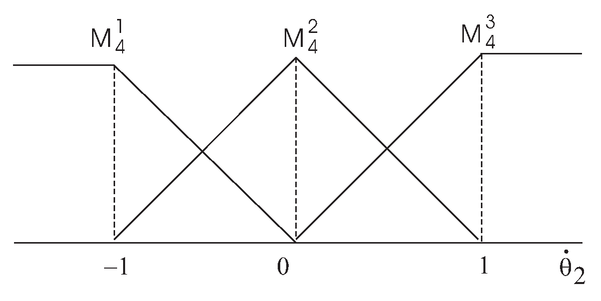
The workspace is defined as follows: θ 1 [ 0 , π ] , θ ˙ 1 [ 1 , 1 ] , θ 2 [ π 2 , π 2 ] , and θ ˙ 2 [ 1 , 1 ] . For this example, we employ five membership functions for the position variables and three for the velocity variables. Figure 3, Figure 4, Figure 5 and Figure 6 display the membership functions for θ , θ ˙ 1 , θ 2 and θ ˙ 2 , respectively.
By applying the methodology described in [29,31], we obtain the following results:
S 1111 : I f x 1 i s M 1 i 1 a n d x 4 i s M 4 i 1 t h e n x ˙ 2 = 2.2816 14.8609 x 1 + 1.2924 x 2 2.1967 x 3 + 0.1681 x 4 + 0.3355 u 1 0.3346 u 2 x ˙ 4 = 8.4921 + 24.2250 x 1 3.1540 x 2 + 0.7544 x 3 + 0.4721 x 4 0.2624 u 1 + 1.1547 u 2 S 4444 : I f x 1 i s M 1 i 4 a n d x 4 i s M 4 i 4 t h e n x ˙ 2 = 1.5761 + 1.7165 x 1 1.7015 x 2 1.6274 x 3 + 1.1794 x 4 + 0.2618 u 1 0.3398 u 2 x ˙ 4 = 6.0187 3.8358 x 1 + 4.1864 x 2 + 8.5766 x 3 2.1167 x 4 0.1041 u 1 + 1.1526 u 2
Using this approximation, the mean square error for the first joint is 0.0016, with a maximum absolute error of 1.1055. For the second joint, the mean square error is 0.0040, with the same maximum absolute error of 1.1055.
The parameter-weighting method ensures that the obtained results represent the best possible approximation of the T-S model as the interval coverage approaches completeness. However, this theoretical limit cannot be fully achieved in practice, as it renders the computation intractable. Nevertheless, this method consistently yields more accurate results than the original T-S modeling approach.
The outputs of the system are the joint angles of the first and second links, denoted by θ 1 and θ 2 , respectively, where
C = 1 0 0 0 0 0 1 0

7.2. Proposed Optimal Controller

The matrix S is defined as follows:
S = 0 1 0 0 0 0 0 1
First, the feedback system matrix must be computed. The linearized system is obtained by applying the minimum least squares method around the equilibrium point defined by
π 2 0 0 0 T
τ 10 τ 20 = 35.525 11.025
The resulting linear model of the system is given by
x ˙ = 0 1 0 0 5.8137 0.0072 0.4226 0.1265 0 0 0 1.0000 7.9809 0.0089 3.4335 0.4205 x ( t ) + 0 0 0.7778 1.5877 0 0 1.5968 4.1704 u ( t )
The selection of the weighting matrices Q and R in the cost function was performed using an iterative trial-and-error approach. This involved systematically varying the elements of the matrices to evaluate their influence on the system’s performance. A commonly adopted strategy in the literature involves choosing Q as a diagonal matrix with relatively large values on the diagonal (e.g., Q = 10000 I ) to emphasize state penalties while setting R as the identity matrix, R = I , to impose a standard control effort penalty. In the context of this study, the weighting matrices were specified as follows:
Q = 1000 0 0 0 0 0 0 1000 0 0 0 0 0 0 1000 0 0 0 0 0 0 100 0 0 0 0 0 0 1000 0 0 0 0 0 0 100 , R = 1 0 0 1
Accordingly, the following optimal controller matrices are obtained:
K = 0 0 23.6613 50.6547 0 0 48.0394 132.7923
A f = 0 1.0000 0 0 32.2124 9.3863 65.1860 16.7827 0 0 0 1.0000 61.5397 14.7298 172.6900 45.9968

7.3. Case Examples

  • Case 1:
The setpoint is set to the state 3 π 4 0 0 0 T starting from the zero initial condition. The transient response of each robot joint is shown in Figure 7.
  • Case 2:
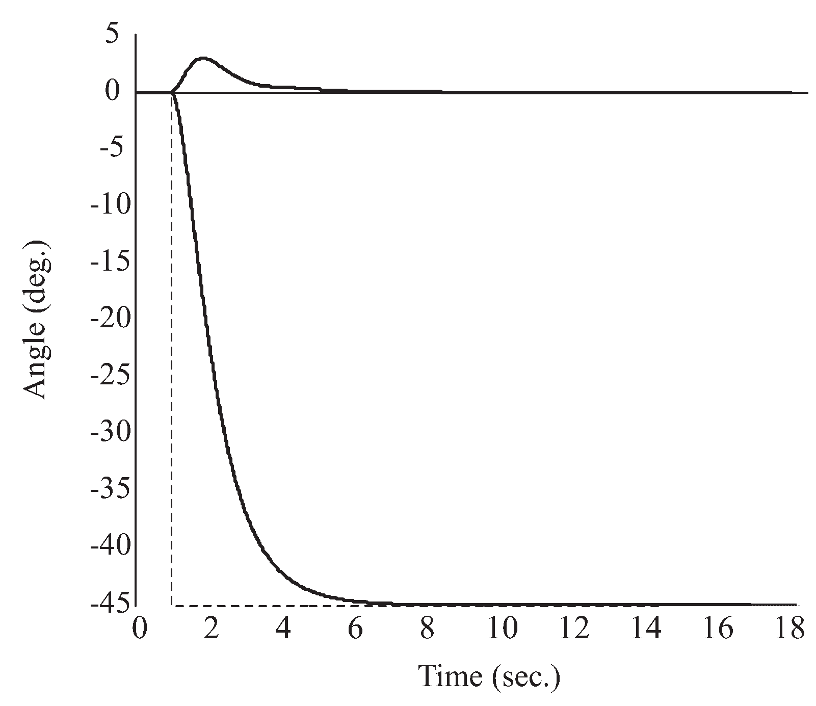
The setpoint is set to the state 0 0 π 4 0 T starting from the zero initial condition. The transient response of each robot joint is illustrated in Figure 8.
  • Case 3:
The setpoint is initially set to 3 π 2 0 0 0 T at 1 s, and then changed to 3 π 2 0 π 4 0 T at 10 s, starting from zero initial conditions. The transient response of each robot joint is shown in Figure 9.
  • Disturbance effect:
The robot is assumed to be subjected to a load of mass p at a certain instant. Accordingly, Equation (31) can be rewritten as follows:
H 11 H 12 H 21 H 22 θ ¨ + h θ ˙ 2 h θ ˙ 1 h θ ˙ 2 h θ ˙ 1 0 θ ˙ + β 1 0 0 β 2 θ ˙ + g 1 g 2 = τ
where θ = [ θ 1 θ 2 ] T denotes the joint angles, τ = [ τ 1 τ 2 ] T represents the input torques at each joint, and
H 11 = m 1 l c 1 2 + I 1 + m 2 ( l 1 2 + l c 2 2 + 2 l 1 l c 2 c o s θ 2 ) + I 2 + p ( l 1 2 + l 2 2 + 2 l 1 l 2 c o s θ 2 ) H 12 = m 2 l 1 l c 2 c o s θ 2 + m 2 l c 2 2 + I 2 + p l 2 2 H 21 = H 12 H 22 = m 2 l c 2 2 + I 2 + p l 2 2 h = m 2 l 1 l c 2 s i n θ 2 + p l 1 l 2 s i n θ 2 g 1 = m 1 l c 1 g s i n θ 1 + m 2 g ( l c 2 s i n ( θ 1 + θ 2 ) + l 1 s i n θ 1 ) + p g ( l 2 s i n ( θ 1 + θ 2 ) + l 1 s i n θ 1 ) g 2 = m 2 l c 2 g s i n ( θ 1 + θ 2 ) + p l 2 g s i n ( θ 1 + θ 2 )
Equation (31) can be expressed in the following compact form:
H ( θ ) θ ¨ + C ( θ , θ ˙ ) θ ˙ + B θ ˙ + g ( θ ) = τ
  • Case 4:
The setpoint is set to 3 π 4 0 0 0 T at 1 s, and then changed to 3 π 4 0 π 4 0 T at 10 s, starting from zero initial conditions. At 20 s, the robot is subjected to an external load of p = 0.5 kg. The transient response of each robot joint is shown in Figure 10.
  • Case 5:
The setpoint is set to 3 π 4 0 0 0 T at 1 s, and then changed to 3 π 2 0 π 4 0 T at 10 s, starting from zero initial conditions. At 20 s, the robot is subjected to a load of p = 0.5 kg and measurement noise in the angle with standard deviation σ = 1 . Figure 11 depicts the transient response of the two-link robot.
  • Case 6:
To further analyze the robustness of the system, the setup from Case 5 is repeated with the measurement noise increased to σ = 2 . The transient response, shown in Figure 12, demonstrates that the system’s behavior remains largely unaffected despite the increased disturbances and noise.
  • Case 7:
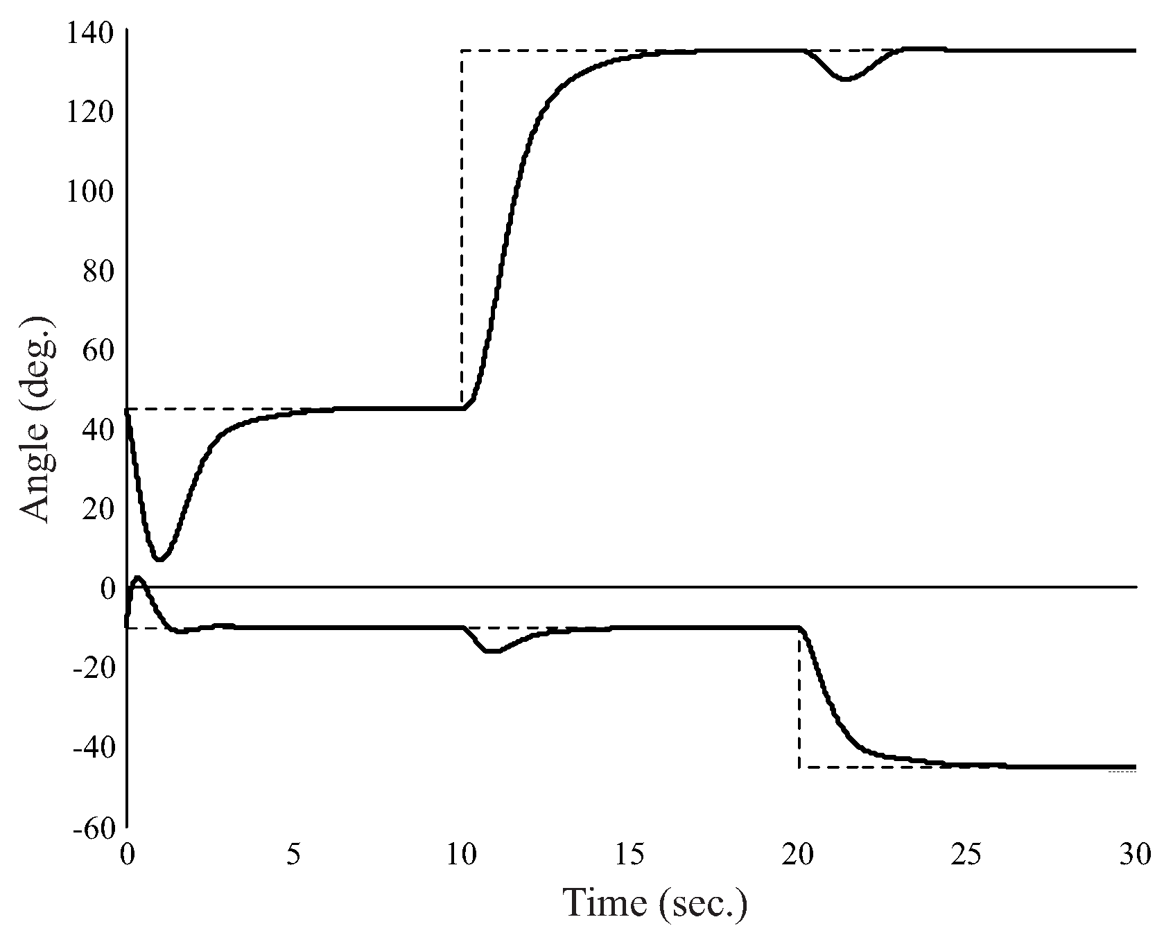
Finally, Figure 13 shows the transient response of the two-link robot starting from non-zero initial conditions, specifically 45 in the first joint and 10 in the second.
The example cases clearly demonstrate that the proposed controller achieves robust and stable performance even in the presence of disturbances, load variations, and measurement noise. It produces a smooth, well-damped transient response while ensuring zero steady-state error.

8. Conclusions

This paper has presented a feedback linearization scheme integrated with Takagi–Sugeno (T-S) fuzzy systems to design a robust controller for nonlinear multivariable systems. The improved T-S modeling approach and the proposed controller construction enable the development of a linearized closed-loop system that is stable from any initial condition and demonstrates strong performance even in the presence of noise and load variations.
A two-link robot was used as a case study to illustrate the effectiveness, accuracy, and robustness of the closed-loop system. Simulation results confirm the smoothness and robustness of the controller, demonstrating that it maintains performance despite disturbances, load changes, and measurement noise. Overall, the controller exhibits well-damped behavior with zero steady-state error.

Author Contributions

Conceptualization, B.M.A.-H. and A.J.; methodology, B.M.A.-H.; software, A.J.; validation, B.M.A.-H. and A.J.; formal analysis, B.M.A.-H.; investigation, B.M.A.-H.; resources, A.J.; data curation, B.M.A.-H.; original draft preparation, A.J.; review and editing, B.M.A.-H. and J.B.R.; visualization, J.B.R.; supervision, B.M.A.-H.; project administration, B.M.A.-H.; funding acquisition, A.J. All authors have read and agreed to the published version of the manuscript.

Funding

This research received no external funding.

Data Availability Statement

The original contributions presented in the study are included in the article; further inquiries can be directed to the corresponding author.

Conflicts of Interest

The authors declare no conflicts of interest.

References

  1. Floares, A. Feedback linearization using neural networks applied to advanced pharmacodynamic and pharmacogenomic systems. In Proceedings of the International Joint Conference on Neural Networks 2005, Montreal, QC, Canada, 31 July–4 August 2005; Volume 1, pp. 173–178. [Google Scholar]
  2. Herníndez-Santiago, J.; Garrido-Meléndez, J.; Escobedo-Trujillo, B.A.; Alcalá-Peréa, G. Exact Feedback Linearization Technique Applied to an Inverted Pendulum Coupled to a DC Motor. In Proceedings of the 2023 IEEE International Conference on Engineering Veracruz (ICEV), Boca del Río, Veracruz, Mexico, 23–26 October 2023; IEEE: Piscataway, NJ, USA, 2023. [Google Scholar]
  3. Swain, N.; Malik, S.; Pati, N. Design and Analysis of Step up Regulator using Exact Feedback Linearization by State Feedback Approach. In Proceedings of the 2021 19th OITS International Conference on Information Technology (OCIT), Bhubaneswar, India, 16–18 December 2021; IEEE: Piscataway, NJ, USA, 2021. [Google Scholar]
  4. Fang, Z.; Yu, Z.; Huang, Q.; Wang, Y.; Gu, X. Research on design and control method of active vibration isolation system based on piezoelectric Stewart platform. Sci. Rep. 2025, 15, 944. [Google Scholar] [CrossRef] [PubMed]
  5. Mihaly, V.; Şuşcă, M.; Birlescu, I.; Sim, S.; Pisla, D.; Dobra, P. Robust Feedback Linearization for Serial Robots. In Proceedings of the 2024 IEEE International Conference on Automation, Quality and Testing, Robotics (AQTR), Cluj-Napoca, Romania, 16–18 May 2024; IEEE: Piscataway, NJ, USA, 2024. [Google Scholar]
  6. Gao, Q.; Liu, L.; Feng, G.; Wang, Y.; Qiu, J. Universal Fuzzy Integral Sliding-Mode Controllers Based on T–S Fuzzy Models. IEEE Trans. Fuzzy Syst. 2013, 22, 350–362. [Google Scholar] [CrossRef]
  7. Sarbaz, M.; Manthouri, M.; Zamani, I. Rough Neural Network and Adaptive Feedback Linearization Control Based on Lyapunov Function. In Proceedings of the 2021 7th International Conference on Control, Instrumentation and Automation (ICCIA), Tabriz, Iran, 23–24 February 2021; IEEE: Piscataway, NJ, USA, 2021. [Google Scholar]
  8. Park, C.-W.; Kang, H.-J.; Yee, Y.-H.; Park, M. Numerical robust stability analysis of fuzzy feedback linearisation regulator based on linear matrix inequality approach. IEE Proc. Control. Theory Appl. 2002, 149, 82–88. [Google Scholar] [CrossRef]
  9. Takagi, T.; Sugeno, M. Fuzzy Identification of Systems and Its Applications to Modeling and Control. IEEE Trans. Syst. Man Cybern. 1985, 15, 116–132. [Google Scholar] [CrossRef]
  10. Zeng, K.; Zhang, N.Y.; Xu, W.L. A comparative study on sufficient conditions for Takagi-Sugeno fuzzy systems as universal approximators. IEEE Trans. Fuzzy Syst. 2000, 8, 773–780. [Google Scholar]
  11. Al-Hadithi, B.M.; Jiménez, A.; Matía, F. Variable Structure Control with Chattering Reduction of a Generalized T-S Model. Asian J. Control. 2012, 15, 155–168. [Google Scholar] [CrossRef]
  12. Gang, F. A survey on analysis and design of model-based fuzzy control systems. IEEE Trans. Fuzzy Syst. 2006, 14, 676–697. [Google Scholar] [CrossRef]
  13. El-Sousy, F.F.M.; Elmorshedy, M.F.; Amin, M.M.; Mohammed, O.A. Robust Adaptive Feedback Linearization Control Using Online Neural-Network Estimators for Uncertain Linear Induction Motor Drive System. In Proceedings of the 2021 13th International Symposium on Linear Drives for Industry Applications (LDIA), Wuhan, China, 1–3 July 2021; IEEE: Piscataway, NJ, USA, 2021. [Google Scholar]
  14. Huang, C.-J.; Li, T.-H.S.; Chen, C.-C. Fuzzy Feedback Linearization Control for MIMO Nonlinear System and Its Application to Full-Vehicle Suspension System. Circuits Syst. Signal Process. 2009, 28, 959–991. [Google Scholar] [CrossRef]
  15. Chung-Cheng, C.; Chao-Hsing, H.; Ying-Jen, C.; Yen-Feng, L. Disturbance attenuation of nonlinear control systems using an observer-based fuzzy feedback linearization control. Chaos Solitons Fractals 2007, 33, 885–900. [Google Scholar]
  16. THSLi, CJHuang, CCChen, Novel fuzzy feedback linearization strategy for control via differential geometry approach. ISA Trans. 2010, 49, 348–357. [CrossRef]
  17. Xiaoshen, L.; Xuehai, Y.; Mingzuo, J.; Chunling, Z. Fuzzy inference modeling method of time-varying system based on TS fuzzy system. In Proceedings of the 2015 12th International Conference on Fuzzy Systems and Knowledge Discovery (FSKD), Zhangjiajie, China, 15–17 August 2015; IEEE: Piscataway, NJ, USA, 2015. [Google Scholar]
  18. Salgado, C.M.; Viegas, J.L.; Azevedo, C.S.; Ferreira, M.C.; Vieira, S.M.; Sousa, J.M.C. Takagi–Sugeno Fuzzy Modeling Using Mixed Fuzzy Clustering. IEEE Trans. Fuzzy Syst. 2016, 25, 1417–1429. [Google Scholar] [CrossRef]
  19. Zeng, X.J. A comparison between TS fuzzy systems and affine TS fuzzy systems as nonlinear control system models. In Proceedings of the 2014 IEEE International Conference on Fuzzy Systems (FUZZ-IEEE), Beijing, China, 6–11 July 2014; IEEE: Piscataway, NJ, USA, 2014. [Google Scholar]
  20. Naizheng, S.; Junmin, L.; Lunle, Y. Adaptive fuzzy control of nonlinear systems based on multiple inputs TS fuzzy bilinear model. In Proceedings of the 31st Chinese Control Conference, Hefei, China, 25–27 July 2012; IEEE: Piscataway, NJ, USA, 2012. [Google Scholar]
  21. Chang-Woo, P. Robust Stable Fuzzy Control via Fuzzy Modeling and Feedback Linearization with Its Applications to Controlling Uncertain Single-link Flexible Joint Manipulators. J. Intell. Robot. Syst. 2004, 39, 131147. [Google Scholar] [CrossRef]
  22. Kim, S.W.; Lee, J.J. Fuzzy control of a class of multivariable nonlinear systems subject to parameter uncertainties: Model reference approach. Int. J. Approx. Reason. 2001, 26, 129–144. [Google Scholar] [CrossRef]
  23. Purwar, S.; Kar, I.N.; Jha, A.N. Adaptive control of robot manipulators using fuzzy logic systems under actuator constraints. Fuzzy Sets Syst. 2005, 152, 651–664. [Google Scholar] [CrossRef]
  24. Labiod, S.; Boucherit, M.S.; Guerra, T.M. Adaptive fuzzy control of a class of MIMO nonlinear systems. Fuzzy Sets Syst. 2005, 15, 59–77. [Google Scholar] [CrossRef]
  25. Song, Z.; Yi, J.; Zhao, D.; Li, X. A computed torque controller for uncertain robotic manipulator systems: Fuzzy approach. Fuzzy Sets Syst. 2006, 154, 208–226. [Google Scholar] [CrossRef]
  26. Tsai, C.H.; Wang, C.H.; Lin, W.S. Robust fuzzy model following control of robot manipulators. IEEE Trans. Fuzzy Syst. 2000, 8, 462–469. [Google Scholar] [CrossRef]
  27. Xu, Y.; Bao, R.; Zhang, L.; Wang, J.; Wang, S. Embodied intelligence in RO/RO logistic terminal: Autonomous intelligent transportation robot architecture. Sci. China Inf. Sci. 2025, 68, 1–17. [Google Scholar] [CrossRef]
  28. Chen, Z.; Zhan, G.; Jiang, Z.; Zhang, W.; Rao, Z.; Wang, H.; Li, J. Adaptive impedance control for docking robot via Stewart parallel mechanism. ISA Trans. 2024, 155, 361–372. [Google Scholar] [CrossRef]
  29. Al-Hadithi, B.M.; Jiménez, A.; Matía, F. A new approach to fuzzy estimation of Takagi-Sugeno model and its applications to optimal control for nonlinear systems. Appl. Soft Comput. 2012, 12, 280–290. [Google Scholar] [CrossRef]
  30. Jiménez, A.; Al-Hadithi, B.M.; Matía, F. An Optimal T-S Model for the Estimation and Identification of Nonlinear Functions. WSEAS Trans. Syst. Control. 2008, 3, 897–906. [Google Scholar]
  31. Jiménez, A.; Al-Hadithi, B.M.; Matía, F. Improvement of Takagi-Sugeno Fuzzy Model for the Estimation of Nonlinear Functions. Asian J. Control. 2012, 14, 320–334. [Google Scholar] [CrossRef]
  32. Louda, S.; Karkar, N.; Seghir, F.; Boutalbi, O. Fuzzy Dynamic Feedback Linearization for Efficient Mobile Robot Trajectory Tracking and Obstacle Avoidance in Autonomous Navigation. Int. J. Robot. Control. Syst. 2025, 5, 881–901. [Google Scholar] [CrossRef]
  33. Yesil, B.; Sahin, S. Real-Time Implementation of a Microcontroller-Based Coupled-TankWater Level Control System with Feedback Linearization and Fuzzy Logic Controller Algorithms. Sensors 2025, 25, 1279. [Google Scholar] [CrossRef]
  34. Al-Ani, F.R.; Lutfy, O.F.; Al-Khazraji, H. Optimal Synergetic and Feedback Linearization Controllers Design for Magnetic Levitation Systems: A Comparative Study. J. Robot Control (JRC) 2024, 6, 22–30. [Google Scholar] [CrossRef]
  35. Al-Hadithi, B.M.; Jiménez, A.; Pérez-Oria, J.; Alonso, L. Optimal Control Using Feedback Linearization for a Generalized T-S Model. In IFIP International Federation for Information Processing 2014, AIAI 2014, Hangzhou, China, 17–20 October 2014; IFIP AICT 436; Springer: Berlin/Heidelberg, Germany, 2014; pp. 466–475. [Google Scholar]
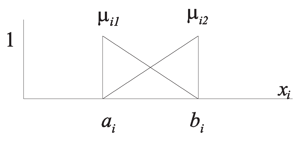
Figure 1. Fuzzy system membership functions.
Electronics 14 03129 g001
Figure 2. Two-link robot.
Electronics 14 03129 g002
Figure 3. Membership functions of θ 1 .
Electronics 14 03129 g003
Figure 4. Membership functions of θ ˙ 1 .
Electronics 14 03129 g004
Figure 5. Membership functions of θ 2 .
Electronics 14 03129 g005
Figure 6. Membership functions of θ ˙ 2 .
Electronics 14 03129 g006
Figure 7. The two-link robot transient response and the final value of 3 π 4 of the first link.
Electronics 14 03129 g007
Figure 8. The two-link robot transient response and the final value of π 4 of the second link.
Electronics 14 03129 g008
Figure 9. The two-link robot transient response and the final values of 3 π 4 and π 4 of the first and second links, respectively.
Electronics 14 03129 g009
Figure 10. The two-link robot transient response and the load effect.
Electronics 14 03129 g010
Figure 11. The two-link robot transient response and the load effect and measurement noise of σ = 1 .
Electronics 14 03129 g011
Figure 12. The two-link robot transient response and the load effect and measurement noise of σ = 2 .
Electronics 14 03129 g012
Figure 13. The two-link robot transient response with initial conditions ( 45 , 10 ).
Electronics 14 03129 g013
Disclaimer/Publisher’s Note: The statements, opinions and data contained in all publications are solely those of the individual author(s) and contributor(s) and not of MDPI and/or the editor(s). MDPI and/or the editor(s) disclaim responsibility for any injury to people or property resulting from any ideas, methods, instructions or products referred to in the content.