Abstract
High-voltage diodes, as key devices in power electronic systems, have important significance for system reliability and preventive maintenance in terms of storage life prediction. In this paper, we propose a hybrid modeling framework that integrates the Long Short-Term Memory Network (LSTM) and Transformer structure, and is hyper-parameter optimized by the Improved Artificial Bee Colony Algorithm (IABC), aiming to realize the high-precision modeling and prediction of high-voltage diode storage life. The framework combines the advantages of LSTM in time-dependent modeling with the global feature extraction capability of Transformer’s self-attention mechanism, and improves the feature learning effect under small-sample conditions through a deep fusion strategy. Meanwhile, the parameter type-aware IABC search mechanism is introduced to efficiently optimize the model hyperparameters. The experimental results show that, compared with the unoptimized model, the average mean square error (MSE) of the proposed model is reduced by 33.7% (from 0.00574 to 0.00402) and the coefficient of determination (R2) is improved by 3.6% (from 0.892 to 0.924) in 10-fold cross-validation. The average predicted lifetime of the sample was 39,403.3 h, and the mean relative uncertainty of prediction was 12.57%. This study provides an efficient tool for power electronics reliability engineering and has important applications for smart grid and new energy system health management.
1. Introduction
High-voltage diodes are core components of modern power electronic systems, which are widely used in energy conversion, electric vehicles, industrial automation, and renewable energy systems, and their reliability directly affects the operational safety and efficiency of power electronic systems, in which high-voltage diodes occupy a key position [1]. The accurate prediction of their storage life remains challenging due to complex degradation mechanisms affected by environmental stresses, electrical load variations, and material aging. Traditional degradation prediction methods mainly rely on simplified physical models or statistical methods, such as the Arrhenius model and the Weibull distribution [2,3], which often fail to capture nonlinear degradation patterns. Traditional degradation prediction methods primarily rely on simplified physical models or statistical approaches. Among these, the Arrhenius model is based on chemical reaction kinetics theory, assuming that the degradation rate exhibits an exponential relationship with temperature. Its mathematical expression is , where represents the failure rate, A is the frequency factor, denotes the activation energy, k is the Boltzmann constant, and T is the absolute temperature. However, this model suffers from the following limitations: (1) Single-stress assumption: it only considers the influence of temperature stress while neglecting the coupling effects of multiple stresses such as voltage and humidity; (2) Linear degradation assumption: it assumes that the degradation process follows linear patterns, failing to describe the nonlinear degradation behaviors commonly observed in actual devices, such as rapid failure phases following initial slow degradation periods; (3) Parameter estimation difficulties: under limited experimental data conditions, the estimation accuracy of key parameters like activation energy is relatively low.
The Weibull distribution model describes the failure probability distribution of devices through shape parameter and scale parameter , with its probability density function expressed as . The main limitations of this model include (1) Static modeling: it cannot reflect the dynamic evolutionary characteristics of degradation processes, making it difficult to capture the time-varying nature of degradation rates; (2) Strict assumption constraints: it requires failure data to strictly follow the Weibull distribution, and when actual degradation processes deviate from this distribution, prediction accuracy significantly decreases; (3) Poor environmental adaptability: model parameters are typically determined under specific experimental conditions, making it difficult to adapt to environmental changes in practical applications.
The common weakness of these traditional methods is their inability to effectively handle the nonlinear, multi-stage, and multi-factor coupling characteristics in high-voltage diode degradation processes. Particularly under small-sample conditions of accelerated aging tests, their prediction accuracy and reliability often fail to meet the requirements of engineering applications. In recent years, deep learning methods have demonstrated strong nonlinear modeling capabilities and made significant progress in the field of remaining useful life (RUL) prediction [4,5]. Recent studies further validate hybrid architectures: He et al. combined Transformer with Kolmogorov–Arnold networks for bearing RUL prediction [6]; Xu integrated attention-LSTM with artificial bee colony optimization for lithium batteries [7].
Among deep learning methods, LSTM networks can effectively deal with the long-term dependency problem in time-series data by virtue of its unique gating mechanism and memory unit structure [8,9]. In recent years, LSTM has been widely used in the field of lifetime prediction. For example, Wang et al. applied LSTM to bearing life prediction and extracted the timing features through a multilayer LSTM network, and the prediction accuracy was improved by 42% compared with that of traditional RNN [10]. Zhang et al. proposed a battery life prediction model based on LSTM-RNN, and introduced the elastic mean-square backpropagation method to perform the adaptive optimization, which enhances the ability of extracting the key timing features, and improves the prediction accuracy significantly [11]. And, the Transformer model has received widespread attention since it was proposed in 2017 for its parallel computing capability and global modeling advantages [12]. Important progress has also been made in the application of Transformer in the field of lifetime prediction. Chen et al. applied Transformer to mechanical device RUL prediction, and through the mechanism of multiple self-attention, to capture degradation sequences in the long-range dependencies, and the prediction accuracy is improved by 15% compared with LSTM [13]. Zhang et al. proposed a fusion model for lithium-electronic battery RUL estimation, which integrates the stacked denoising self-encoder (SDAE) and Transformer model, and improves the accuracy compared with the traditional recursive model [14]. Zhang et al. designed a self-attention Transformer for multi-feature battery degradation [15] and Wang et al. proposed multivariate dynamic embedding for industrial time series [16].
And, the LSTM-Transformer hybrid model framework proposed in recent years combines the local time-series modeling capability of LSTM and the global dependency capture advantage of Transformer, which shows significant potential in time-series prediction tasks, especially in the field of RUL prediction, which has been widely studied. Lu et al. proposed an LSTM-Transformer hybrid architecture fuel cell lifetime prediction model, which can not only capture the local features of fuel cell performance degradation, but also effectively simulate the long-term degradation trend of the fuel cell by deeply fusing the two neural networks, improving the prediction accuracy and generalization ability [17]. In addition, Pentsos et al. proposed an LSTM-Transformer model designed for power load prediction, which utilizes the advantages of the LSTM and Transformer model to achieve more accurate and reliable prediction of power consumption [18]. These studies show that the hybrid LSTM-Transformer modeling framework has significant advantages in dealing with complex timing prediction tasks, and is able to effectively deal with challenges such as nonlinear degradation patterns, multimodal data, and so on.
However, the existing research on the LSTM-Transformer hybrid architecture has the following limitations: (1) the limitation of the application field and the lack of adaptability of degradation mechanism—existing research is mainly concentrated in the fields of mechanical equipment, power batteries, and so on, and research into the degradation prediction of semiconductor devices such as high-voltage diodes is relatively limited, while the degradation mechanism of high-voltage diodes is essentially different from mechanical wear or battery capacity degradation. Different from the gradual wear of mechanical equipment or the monotonous degradation of battery capacity, the degradation of high-voltage diodes presents multi-stage nonlinear characteristics: slow drift in the initial stage, accelerated degradation in the middle stage, and sharp failure in the later stage. The existing series parallel fusion mechanism cannot adaptively identify and model this complex multi-stage degradation mode, and lacks the targeted feature extraction and weight adjustment mechanism for different degradation stages, resulting in significant differences in the prediction accuracy of different degradation stages; (2) The insufficient processing capacity of small samples—the accelerated aging test usually can only obtain limited sample data. Existing research work is mainly based on large sample datasets (usually containing thousands to tens of thousands of sample points), while accelerated aging test of high voltage diode can only obtain dozens to hundreds of degradation data points due to high cost, long cycle and limited number of equipment. Under such small sample conditions, the traditional LSTM transformer hybrid structure is prone to overfitting, which cannot fully extract the key degradation features in sparse data, and lacks effective regularization and data enhancement strategies to improve the generalization ability of the model, Pan et al. addressed this via knowledge-based data augmentation [19]; (3) The fusion strategy is singular and lacks uncertainty quantification—most existing studies use simple series parallel fusion or weighted average, lack a specialized fusion mechanism design for degradation prediction tasks, cannot effectively integrate local time series information and global dependencies, and lack quantification and confidence evaluation mechanisms for prediction uncertainty.
Compared with existing research on the hybrid structure of LSTM transformer, there are significant differences in the architecture design and fusion strategy of this research: the existing research mostly adopts the simple series structure (LSTM before transformer) or the parallel structure (two paths are calculated independently and then fused directly), while the two-path residual connection mechanism proposed in this research not only maintains the independence of the two modules, but also realizes the effective transmission of deep features and the optimization of gradient flow through residual connection. In addition, existing studies mostly rely on data enhancement or simple regularization techniques when processing small sample data, while this study can more effectively learn and generalize degradation patterns under limited sample conditions through specially designed residual path and multi-scale feature extraction mechanism. In terms of uncertainty processing, the traditional LSTM transformer hybrid model mainly focuses on the prediction accuracy and lacks the systematic quantification of the prediction confidence. This study provides a richer feature representation basis for the subsequent uncertainty quantification through the feature separation of the dual path architecture.
Based on the above analysis, the difference between the LSTM-Transformer hybrid architecture proposed in this study and previous studies is that for the multi-stage nonlinear degradation characteristics of high-voltage diodes, a dual path residual connection mechanism for degradation stage perception is designed. Through the adaptive fusion of local time sequence path and global attention path, it can better integrate different scales of time sequence information and global correlation, and flexibly capture relevant features according to the characteristics of the degradation stage.
Artificial Bee Colony (ABC) algorithm is a swarm intelligence optimization algorithm inspired by the foraging behavior of honey bees, proposed by Karaboga et al. in 2005, which has the advantages of few parameters and fast convergence [20]. In the field of deep learning hyper-parameter optimization, the ABC algorithm shows unique advantages. Erkan et al. compared the performance of ABC, particle swarm optimization (PSO), and genetic algorithm (GA) in neural network optimization, and found that ABC has a significant advantage in parameter space exploration efficiency [21]. Lamjiak et al. proposed an improved ABC algorithm that enhances the traditional ABC algorithm by including neighboring food sources of the parameters to enhance the discovery phase of traditional ABC, which enhances the search capability to find the best solution and improves the optimization efficiency [22]. These studies provide an important theoretical and practical foundation for the improved ABC algorithm (IABC) proposed in this study.
Despite the significant progress of deep learning methods in the field of life prediction, the application of these methods to high-voltage diode life prediction still faces many challenges, such as the accurate modeling of complex degradation patterns (especially in the case of small samples), the inefficiency of hyper-parameter optimization, and the insufficient quantification of prediction uncertainty, etc., and the feature extraction and generalization capabilities of existing studies in the field of high-voltage diodes, especially in the case of accelerated aging small samples, still need to be strengthened. To address these challenges, this study proposes a hybrid LSTM-Transformer model framework based on improved artificial bee colony algorithm (IABC) optimization. The core contributions of this framework are (1) constructing and optimizing the LSTM-Transformer hybrid model framework for high-voltage diode degradation prediction. In this study, a two-path residual linkage mechanism is carefully designed to deeply optimize the fusion of the local timing detail capturing the capability of LSTM and the global context-dependent modeling capability of the Transformer. Through the specific fusion strategy, this method fully retains key local dynamic information and integrates global semantic features under limited sample conditions, which significantly improves the robust feature extraction capability and the portrayal effect of nonlinear degradation laws under high noise and complex backgrounds, and provides theoretical and algorithmic support for accurate lifetime prediction; (2) developing optimization algorithms for parameter type sensing. The model hyperparameters are efficiently optimized through strategies such as differential neighborhood search, structural constraints processing and logarithmic space optimization; (3) A multi-method lifetime prediction framework incorporating deep learning trend prediction, stochastic process fluctuation modeling, and statistical extrapolation is constructed, and the prediction uncertainty is quantified.
This study provides high-precision solutions for the reliability assessment of high-voltage electronic devices, which is valuable for the design of smart grids and new energy systems.
2. Construction of the IABC-LSTM-Transformer Model
2.1. Principles of LSTM and Transformer Models
LSTM realizes the selective memory and forgetting of information through cell state and three gating units, namely the forgetting gate, input gate, and output gate. Its core mathematical expression is as follows:
where are the values of the respective gating units; are the weight matrices of the gating units; is the matrix composed of the output at the previous time step and the current input; are the respective bias terms and is the sigmoid function.
The final output at the current time step is determined by an additional sigmoid layer and the transformed cell state via tanh, as follows:
The above mechanism enables LSTM to retain important information and filter out irrelevant content, effectively addressing the long-term dependency problem. The cell structure of the LSTM model is shown in Figure 1.
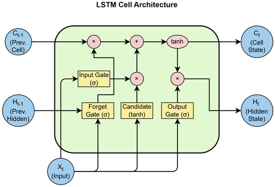
Figure 1.
Cell structure of LSTM model.
Figure 1 shows the cell structure of the LSTM model, illustrating the gating mechanisms (the forget gate, input gate, output gate) and cell state. This structure enables capturing long-term dependencies in degradation sequences, which is critical for modeling the multi-stage failure behaviors of high-voltage diodes.
The Transformer model was proposed by Vaswani et al. in 2017 [12], the core of the Transformer model is a multi-head self-attention mechanism that captures sequence global dependencies. In the multi-head self-attention module, the key vector Q, the weight vector V and the query vector K are computed as
where f is the input sequence, and are trainable projection matrices. Using the above results, the scaled dot-product attention is computed as follows:
where is the dimension of the key vector, and the division by prevents excessively large values when computing the softmax. The softmax function normalizes the attention scores to sum to 1. To focus on information from different positions and representation subspaces, H parallel attention heads are used, and the multi-head attention mechanism is calculated as
where is a learnable weight matrix.
Finally, the outputs of the individual heads are spliced and integrated through a linear layer. The multi-head attention mechanism is able to focus on the different parts of the input sequence at the same time to capture rich semantic information. The structure of the Transformer model is shown in Figure 2.
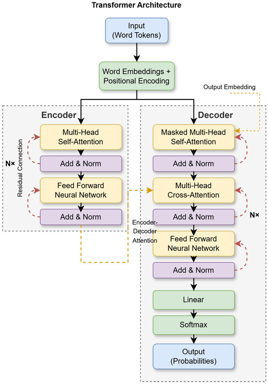
Figure 2.
Structure of the Transformer model.
Figure 2 shows the architecture of the Transformer model with multi-head self-attention and positional encoding. The global dependency modeling capability complements LSTM’s local feature extraction, forming the core of the hybrid framework for high-precision degradation prediction.
2.2. Artificial Bee Colony Algorithm Optimization Framework
The artificial bee colony (ABC) algorithm is a swarm intelligence optimization algorithm that simulates the foraging behavior of bees. Focusing on the complex characteristics of the hyperparameter space of LSTM-Transformer hybrid model that contain different types of parameters (integer, continuous, and coupling constraints), this study proposes an improved ABC (IABC) algorithm for optimization [23,24]. The design of this IABC algorithm draws on the framework of standard ABC and makes adaptive improvements for the characteristics of deep learning hyperparameters, which are mainly reflected in the following aspects:
- Parameter type-aware neighborhood search strategy. Differentiated perturbation mechanisms are used for different types of hyperparameters.For integer parameters such as the number of LSTM units and attention heads, the algorithm adopts an integer value mutation mechanism based on the current solution neighborhood. Firstly, calculate the disturbance intensity based on the range of parameter values and the current population diversity, and then generate an integer offset around the current value. The disturbance intensity will dynamically adjust with the change in population diversity: when the population diversity is low, increase the disturbance amplitude to help the algorithm jump out of the local optimal region; When the diversity is high, reduce the disturbance amplitude for refined search. Simultaneously set up a boundary-checking mechanism to ensure that the generated integer parameters are always within the predefined valid range.For continuous parameters, the algorithm adopts different processing strategies based on the numerical characteristics of the parameters. For parameters with large numerical ranges such as learning rate, searching directly in the original space may result in small numerical regions being ignored, as their effective values may span multiple orders of magnitude (such as 0.0001 to 0.1). Therefore, the algorithm performs perturbation search in the logarithmic space of the learning rate, first converting the current learning rate to the logarithmic domain, adding Gaussian noise to the logarithmic space, and then converting back to the original scale. This strategy enables the algorithm to explore learning rate values of different orders of magnitude more evenly, avoiding search bias towards larger values.For other continuous parameters such as dropout rate, due to their relatively fixed range of values and uniform distribution, the algorithm adopts a standardized Gaussian perturbation mechanism. The disturbance amplitude is normalized according to the range of parameter values to ensure that the disturbances of different parameters have similar relative strengths. At the same time, considering the physical meaning of the parameters, such as the dropout rate must be between 0 and 1, the algorithm will automatically perform boundary constraint processing.For special integer parameters such as batch size, as they usually take a power of 2 to optimize the GPU memory usage, the algorithm has specifically designed a power search strategy to select from candidate power values instead of searching in a continuous integer space.Parameter generation and tuning for structural constraint perception. For the constraint that must be satisfied between the number of attention heads and the dimension of the hidden layer that the dimension is divisible by the number of heads, the algorithm ensures that the selected combination of heads and dimensions is valid when generating and updating these parameters. For example, when randomly generating parameters, the dimension is prioritized and then selected from the valid number of heads; during neighborhood search, if the dimension or number of heads is adjusted, a linkage adjustment is made to maintain the constraint, which avoids model training failure or performance degradation due to invalid parameter combinations.In the attention mechanism of deep learning models, maintaining specific structural constraints is crucial for model stability and performance. The IABC algorithm provides an intuitive constraint processing method for attention parameters. Specifically, when generating or modifying parameters, the algorithm ensures that the hidden layer dimension can always be divided by the number of attention heads, which is a necessary condition for the normal operation of multi-head attention mechanisms. This algorithm implements this constraint through a practical processing mechanism: during the parameter initialization phase, the algorithm first selects valid dimension values, then identifies all attention head values that can divide the dimension, and randomly selects them; In the process of neighborhood search, when the dimension or number of heads needs to be adjusted, the algorithm maintains the mathematical relationship between them through a linkage mechanism to ensure that the generated parameter combinations are always effective. This constraint-aware parameter generation avoids the algorithm exploration of invalid parameter combinations, thereby preventing model training failures and significantly improving optimization efficiency and reliability.Log space search for a learning rate. For parameters such as learning rate, they usually vary greatly in order of magnitude, and learning rates often span multiple orders of magnitude (such as from to ), making uniform exploration in linear space difficult. The IABC algorithm adopts a logarithmic space exploration strategy, providing more balanced coverage across different scales. Perturbation and search in its logarithmic space (log10)are performed where the learning rate is first converted into a logarithmic, Gaussian perturbation is performed on the logarithmic scale, and then converted back to the original scale. This strategy enables the algorithm to explore the learning rate values of different orders of magnitude more evenly, improving the efficiency of finding appropriate learning rates and avoiding excessive focus on larger or smaller values when searching in the original linear space. When generating or perturbing learning rate values, IABC converts the learning rate to a logarithmic scale (log10 space) for operation, where equal distances represent equal ratios rather than absolute differences. The algorithm perturbs the numerical values with Gaussian noise, allowing for proportional changes, and then converts the perturbed values back to the original scale through exponential operations. This method allows the algorithm to explore both subtle adjustments and large-scale changes simultaneously without introducing complex formulas, avoiding falling into the region of diminishing returns when dealing with minima in linear space. Experimental results have shown that this method can consistently discover appropriate learning rates in different model configurations.
The mathematical model of the innovative optimization framework designed in this study for deep learning hyperparameter characteristics can be expressed as follows:
where represents the i-th candidate solution (nectar source position), is the diversity factor and is the search range ratio (set to 0.2), (continuous parameter disturbance intensity), (learning rate disturbance intensity).
The fitness function uses the inverse of the prediction error:
The inverse of the prediction error is chosen due to the reasonableness of the numerical mapping, and the smaller prediction error means a better model performance, but the direct use of the error as the fitness will lead to the reverse optimization problem of “the smaller the better”. After taking the inverse, the smaller the error, the larger the fitness value, which is in line with the basic principle of the artificial bee colony algorithm that the larger the fitness, the better [25]. And, compared with other transformations (e.g., exponential transformation), the inverse operation has less computational overhead, and when the prediction error is close to 0, there is no risk of numerical overflow, although the inverse value becomes large [26], which is especially important in deep learning optimization. In addition, the inverse function provides a smaller optimization step when the error is large and a larger optimization step when the error is small, and this adaptive property helps the algorithm maintain a suitable search intensity at different stages.
Compared with the standard ABC algorithm, the IABC proposed in this study makes key improvements to adapt to the needs of deep learning hyper-parameter optimization in the following aspects: firstly, the standard ABC usually adopts a uniform neighborhood search strategy, while the IABC designs specific updating rules for different parameter types (integer, continuous, and structural constraints), which, as mentioned earlier, are more in line with the actual characteristics of deep learning model parameters; second, dynamic variation amplitude adjustment based on population diversity is introduced, aiming to better balance global exploration and local exploitation, while the perturbation amplitude of the standard ABC is usually fixed or simply varies with the number of iterations; and again, logarithmic spatial search is used for parameters such as learning rate, which improves the efficiency of searching for a large range of parameters. Although a direct parallel experimental comparison of IABC with other optimization algorithms (e.g., standard ABC, PSO, GA, or Bayesian optimization) is not conducted in this study, these targeted improvements are intended to enhance the search performance and convergence speed in complex, high-dimensional, constraint-containing, deep learning hyper-parameter spaces, resulting in better model configurations. In this study, the hyperparameters (e.g., number of LSTM units, learning rate, etc.) of the “LSTM-Transformer hybrid model with base parameters”, which are used to compare the performance with the IABC optimization model, are fixed values based on commonly used configurations in the literature and a small number of preliminary exploratory experiments, and have not been systematically optimized. Aiming to verify the optimization gain of the IABC algorithm, according to the obtained training results, the IABC algorithm proposed in this paper is able to continuously improve the adaptation degree during the iteration process, which indicates that it has an effective search capability. Future research can further conduct exhaustive comparative experiments to quantify the effects of these improvements.
2.3. IABC-LSTM-Transformer Hybrid Architecture
In this study, we design the hybrid model framework that fuses the advantages of LSTM and Transformer. The architecture achieves deep fusion through residual connections and consists of four core modules: sequence input layer, LSTM encoder, self-attention module, and LSTM decoder. The IABC-LSTM-Transformer hybrid model framework is shown in Figure 3.
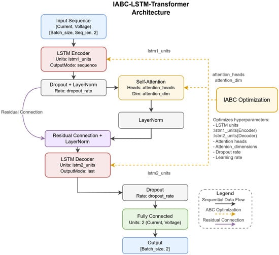
Figure 3.
IABC-LSTM Transformer hybrid model framework.
Figure 3 shows the proposed IABC-LSTM-Transformer hybrid framework. The dual-path residual connections (dashed lines) integrate local temporal features from LSTM and global dependencies from Transformer, enhancing feature fusion and mitigating gradient vanishing. IABC optimizes hyperparameters marked in yellow.
As shown in Figure 3, one of the core innovations of this study lies in the introduction of a two-path residual connection. Specifically, the output sequence of the LSTM encoder (lstm1), after layer normalization, is divided into two paths: one path is directly passed to the subsequent addition layer through a jump connection; the other path enters the self-attention module for global feature enhancement. At the addition layer, these two path features—the original local temporal features and the global features enhanced by the attention mechanism—undergo element-level additive fusion. This design aims to (1) retain the original local timing information to prevent it from being lost in the deep network; (2) effectively incorporate the global context information so that the model can utilize the two features simultaneously for subsequent processing; and (3) effectively mitigate the gradient vanishing problem that may occur in the training of the deep network by providing a “shortcut”. Subsequently, the fused features are normalized by one layer and fed into the LSTM decoder (lstm2) to integrate the multi-scale features and further improve the prediction accuracy. To prevent overfitting, the model introduces Dropout and L2 regularization mechanisms to enhance the generalization ability. Ultimately, the features are mapped into the predicted values of maximum reverse current and highest forward peak voltage through the fully connected layer.
This hybrid model is mainly used to learn and predict the time series of key degradation parameters (maximum reverse current and maximum forward peak voltage) of high-voltage diodes during accelerated aging. After obtaining the short-term prediction sequences of these degradation parameters, this study further employs a fusion prediction strategy to infer the final storage life of the device, which integrates the short-term trend prediction of the present hybrid model framework, the stochastic fluctuation modeling based on the Wiener process, and the statistical extrapolation based on the robust degradation slopes of the historical data. Specific details are described in Section 4.4.1.
In addition, this study utilizes the Improved Artificial Bee Colony Algorithm (IABC) to optimize the model hyperparameters, including key parameters such as the number of LSTM units, the number of attentional heads, the attentional dimensions, the dropout rate, and the learning rate, etc., which ensures that the model is adaptable to different samples. The optimization results show that the optimal hyperparameter configuration significantly improves the model performance, with the average MSE of the test set reduced by 48.1% and the R2 improved by 11.3%, and the specific improvement effects will be analyzed in detail in Section 4.2. By combining an innovative hybrid modeling framework, an efficient hyperparameter optimization strategy, and a multi-method fusion prediction framework, the model provides a high-precision solution for high-voltage diode storage life prediction.
3. Dataset Description
3.1. Accelerated Storage Test Design
In this study, an accelerated test program conforming to the requirements of GJB 548C was designed with reference to relevant standards. The study takes MSL128 ultra-high frequency high-voltage diodes (4–8 kV, 100 mA forward current, ≤100 ns reverse recovery time), whose operational temperature range spans −40 °C to +120 °C with storage limits at −60 °C/+175 °C as the test object (shown in the upper part of Figure 4). Material analysis reveals moisture-sensitive epoxy molding compounds and corrosion-resistant Cu-Mo leadframes, explaining their high humidity sensitivity (>85% RH accelerates ionic contamination) but temperature cycling tolerance. Field data analysis [27] identified maximum reverse current (MRC) and peak forward voltage (PFV) as key degradation indicators—with baselines ≤ 2.0 A @25 °C and ≤15 V @100 mA, respectively, directly sourced from manufacturer specifications.
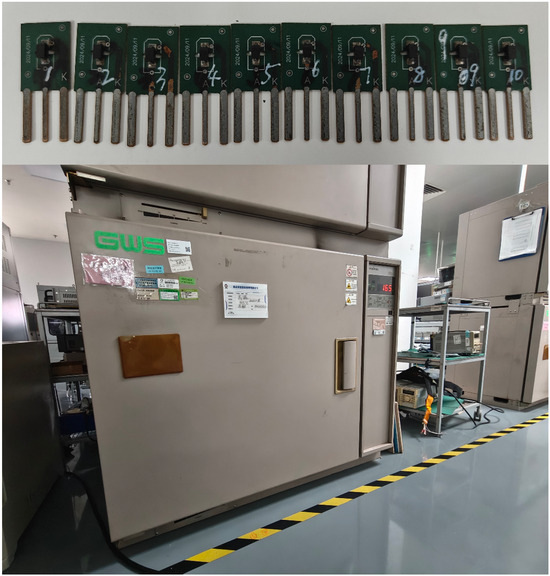
Figure 4.
MSL128 ultra-high frequency high-voltage diodes samples and schematic diagram of HAST test chamber and test environment.
To simulate humid aging, constant highly accelerated stress testing (HAST) was conducted in a GJB 548C-compliant chamber (shown in the below part of Figure 4) at 110 ± 0.5 °C/85 ± 2% RH. Ten MSL128B samples underwent 2016 h exposure with 32 h measurement intervals. Strict protocol enforced: (1) 48 h pre-conditioning at 23 °C/55% RH; (2) Active preheating to 110 °C before HAST; (3) 24 h recovery at 23 ± 3 °C before measurements. Failure thresholds were set at MRC > 2.0 A (indicating junction leakage from moisture ingress) and PFV > 15.0 V (suggesting bond-wire degradation), triggering termination upon >50% cumulative failure. Samples were tested within 48 h post-recovery to minimize environmental drift. Considering epoxy delamination variability, degradation data for each sample was modeled independently to capture device-specific aging trajectories.
Figure 4 shows the ten MSL128 ultra-high-frequency high-voltage diode samples used in the HAST tests and schematic of the HAST chamber (110 °C/85% RH) compliant with GJB 548C. These validate the experimental setup for accelerated aging data collection.
Prior to testing, the devices were stored in a controlled environment at a temperature of 22–25 °C and a relative humidity of 45–64%, and were preheated prior to the start of testing to ensure that each device under test reached the specified temperature. During the test, the devices are removed from the high-temperature and high-humidity environment within 24 h prior to each test and placed under standard test conditions (23 ± 3 °C) for recovery. Tests need to be completed within 48 h from 2 h after the device temperature is restored to room temperature to minimize the impact of environmental changes on the measurement results. The test equipment includes a 370B plotter and a semiconductor parameter analyzer for the accurate measurement of maximum reverse current and maximum forward peak voltage. Considering the individual variability among the samples, this study analyzes and models the degradation data of each sample independently to capture device-specific degradation patterns and aging characteristics, providing a reliable data base for subsequent prediction model construction.
3.2. Data Preprocessing and Feature Extraction
Data preprocessing has an important impact on the performance of deep learning models. To ensure the data quality and the effectiveness of model training, this study systematically preprocesses the collected data in the following steps: (1) data cleaning and calibration to eliminate invalid or erroneous data and ensure the integrity of the dataset; (2) statistical analysis to extract the key statistical features and degradation trend features to provide multidimensional information for the model; and (3) outlier processing and selective smoothing, where, firstly, an outlier is identified by using a method based on the percentile and a certain range of multipliers to initially identify potential outliers, and replace the points beyond the threshold using a median based on non-outliers to reduce the interference of extreme values on model training. Second, a selective smoothing strategy was used to address possible sharp short-term fluctuations in the data: the logarithmic rate of change between data points was calculated to identify points with excessive rates of change, and a simple three-point averaging filter (the current point and the points before and after it) was applied to these points instead of the global smoothing of the entire series, aiming to preserve the main degradation trends while suppressing local noise. (4) Data normalization, which normalizes the degenerate data to the range of [0.1, 1], eliminates the magnitude differences while ensuring that the inputs are positive, which is beneficial for certain subsequent activation functions (e.g., logarithmic correlation) or avoiding computational problems such as division by zero, logarithmic negativity, etc., and helps to improve the stability of the model training. (5) Sequence sample construction, using the sliding window method (the window size is set to 8, and the step size is 1) to construct the time series input data. The choice of window size 8 is based on preliminary experiments and experience, aiming to capture local dependencies with sufficient time span, while avoiding too long sequences leading to reduced computational efficiency and increased risk of overfitting. (6) Dataset partitioning and cross-validation, the 8:2 ratio partitioning of the training and test sets, and 10-fold cross-validation was used to evaluate the model performance.
The statistical characteristics of the degradation data for each sample are shown in Table 1, including the mean, standard deviation and degradation trend coefficients for the maximum reverse current and the highest forward peak voltage. By analyzing the differences between the samples, the diversity of device degradation behaviors can be found, for example, the current degradation rate is higher in some samples, while the voltage changes are smoother. These features provide an important basis for subsequent models to capture individual differences.

Table 1.
Statistical characteristics of the degradation data for each sample.
4. Experimental Results and Analysis
4.1. Performance Evaluation Metrics
In this study, the model performance was comprehensively evaluated using four indicators: mean square error (MSE), root mean square error (RMSE), mean absolute error (MAE), and coefficient of determination (R2). A smaller MSE, RMSE, and MAE indicate better model performance, and a larger R2 indicates better model performance. The formulas are, respectively:
where n is the number of samples, is the true value, is the predicted value, and is the mean of true values. These metrics assess the model prediction performance from different perspectives, providing clear directions for model improvement.
4.2. Analysis of the IABC Optimization Effect
4.2.1. IABC Hyperparameter Optimization Effect
To address the complexity of the hyperparameter space of the hybrid model, the Improved Artificial Bee Colony Algorithm (IABC) proposed in this study significantly improves the optimization efficiency through innovative mechanisms such as adaptive integer variation, structural constraints perception, and logarithmic space search. The sample hyperparameter search space as well as the optimal hyperparameters are shown in Table 2.
Table 2.
Search range for each hyperparameter and optimized hyperparameter values.
The IABC optimization tailors hyperparameters to individual degradation dynamics by adapting to sample-specific failure mechanisms. For LSTM Encoder Units (32–256), higher values (Sample 4: 69 units) model nonlinear degradation in moisture-sensitive samples (current degradation rate 0.0029 A/h), while lower values (Sample 7: 20 units) suffice for stable devices with monotonic aging. Attention heads (1–8) resolve multi-stage failures: Sample 9’s voltage fluctuations (std. 0.1746 V) require two heads to capture phase transitions, contrasting with Sample 10’s steady decay (1 head). Attention dimension (32–256) scales with feature complexity—Sample 5’s accelerated degradation (high current std 0.2330 A) demands larger dimensions (64) to encode abrupt changes, validated by its divisible pair with heads (64 ÷ 2 = 32). LSTM decoder units (32–256) correlate with prediction horizon; long-life samples (Sample 8: low degradation rate 0.0031 A/h) need deeper decoders (40 units) to extrapolate slow degradation. Dropout rate (0.1–0.5) counters overfitting in noisy regimes: Sample 1’s high data variance (current std. 0.1608 A) uses 0.3426 dropout for regularization. Logarithmic learning rate (0.0001–0.01) stabilizes training—Sample 7’s high rate (0.0100) prevents gradient vanishing during sharp failure events. This physics-aware optimization, enabled by IABC’s type-specific search (Section 2.2), reduces the prediction uncertainty by 12.57% and MSE by 48.1%.
Specifically, during the hyperparameter optimization of the 10 samples, as shown in Figure 5, the best fitness of each sample during the IABC iteration was steadily increased from an initial mean value of 28.62 to a final mean value of 45.23 at the end of the iteration, which indicates that the average increase in the best fitness of all the samples reached about 58.0%. At the same time, the average fitness of the entire population also increased from about 17.03 at the beginning to about 29.28 at the end, which represents an average increase of about 71.9%. These results initially show the effectiveness of the IABC algorithm in searching for more optimal hyperparameter combinations. It is worth noting that the exact value and percentage of improvement of the fitness depend on the definition of the fitness function, but its growth trend reflects the convergence ability of the optimization algorithm. Moreover, there are significant differences in the optimization effects of different samples, which reflect the necessity of the personalized optimization and the adaptive nature of the IABC algorithm. These data optimization effects fully demonstrate the excellent search performance of IABC algorithm in complex hyperparameter space. The IABC optimization process is shown in Figure 5. The horizontal axis is the number of iterations (1–30), the vertical axis of Figure (a) is the average best fitness of 10 samples, and the vertical axis of Figure (b) is the average population fitness. The curves show the overall convergence trend and optimization effect of the IABC algorithm, reflecting the search efficiency and stability of the algorithm in the iteration process.
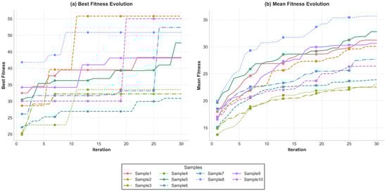
Figure 5.
IABC optimization process.
Figure 5 shows the convergence curves of IABC optimization: (a) Best fitness values over iterations; (b) Population fitness trends. The 58% fitness improvement confirms IABC’s efficacy in hyperparameter search for complex deep learning models.
The IABC algorithm significantly improves model performance. Compared to the model with base parameters, the IABC-optimized model improves the average R2 on the 10-fold cross-validation set from 0.892 to 0.924 (a 3.6% improvement), reduces the average MSE from 0.00574 to 0.00402 (a 33.7% improvement), reduces the average MAE from 0.0489 to 0.0422 (a 13.9% improvement), and reduces the average RMSE decreased from 0.0688 to 0.0593 (14.4% improvement). Statistical significance was verified by a t-test, and the optimized model showed a significant improvement in prediction accuracy on the test set: the average MSE was reduced from 0.00636 to 0.00322 (48.14% improvement, p = 0.0110 < 0.05), the average MAE was reduced from 0.0587 to 0.0391 (33.4% improvement, p = 0.0013 < 0.01), and the mean RMSE decreased from 0.0757 to 0.0512 (32.36% improvement, p = 0.0044 < 0.01). Figure 6 and Figure 7 present in detail the optimization of the Improved Artificial Bee Colony Algorithm (IABC) on 10 high-voltage diode samples cross-validated with the test set.
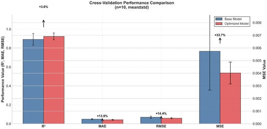
Figure 6.
Comparison of cross-validations.
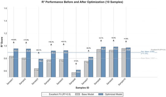
Figure 7.
Comparison of test sets.
Figure 7 shows the comparison of R2 metrics on independent test sets for the model before and after IABC optimization.
Figure 6 shows the comparison of various performance metrics (R2, MSE, MAE, RMSE) of the model on the cross-validation set before and after IABC optimization.
To validate the performance of IABC, comparative experiments were conducted with Bayesian optimization and particle swarm optimization (PSO) algorithms on identical optimization tasks. The experimental results across 10 samples runs demonstrate that IABC consistently outperformed both baseline methods. Specifically, IABC achieved a mean best fitness of 44.48 (±9.50), significantly higher than Bayesian optimization (29.50 ± 6.04) and PSO (26.79 ± 5.44). Moreover, IABC exhibited superior computational efficiency with a mean optimization time of 12.07 s (±0.80), compared to 18.10 s (±0.90) for Bayesian optimization and 15.14 s (±0.63) for PSO. These results empirically confirm the theoretical advantages of IABC in handling complex hyperparameter optimization tasks for deep learning models. Figure 8 illustrates the performance comparison between IABC, Bayesian optimization, and PSO across 10 independent runs. And, as described in Section 2.2, IABC is theoretically able to handle the complex hyperparameter space of deep learning models more efficiently than standard ABC by introducing mechanisms such as parameter type-aware search strategies, structural constraints handling, and log-space search for learning rate.
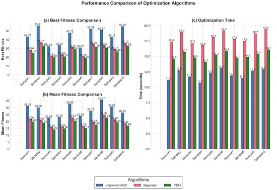
Figure 8.
Performance comparison of optimization algorithms.
Figure 8 shows the algorithm benchmarking, highlighting the 33.7% MSE reduction and IABC’s superiority over Bayesian/PSO methods.
4.2.2. Verification of Generalizability
In order to further verify the generalization ability of the IABC optimization algorithm, this study applies the optimization algorithm to the external validation dataset of NMOS tubes with model number C500N8C3-2. The NMOS tubes and the high-voltage diodes are from the same batch of test samples, and all the test procedures are consistent. The sensitive parameters are zero gate voltage leakage current and gate threshold voltage. The same base model and IABC optimization flow as in the high-voltage diode dataset are used on this external dataset to evaluate the performance of the optimization algorithm under different data sources and possible differences in data distribution. The experimental results show that the IABC-optimized model exhibits a significant performance improvement on the 10-fold cross-validation set compared to the model with base parameters: the R2 on the 10-fold cross-validation set improves from 0.950 to 0.968 (a 1.7% improvement), the mean squared error MSE improves by 36.2% (from 0.00208 to 0.00133), the mean absolute error MAE decreased by 21.5% (from 0.0361 to 0.0284), and the root mean square error RMSE decreased by 19.1% (from 0.0425 to 0.0344). The overall improvement in these metrics indicates that the IABC optimized model not only performs well on the high-voltage diode dataset, but also achieves considerable performance gains on external datasets. This result strongly demonstrates that the IABC optimization is not merely an overfitting phenomenon for a specific dataset, but rather, the optimization process learns more robust and adaptive model parameters to maintain excellent prediction ability under different data distributions. In summary, through the multi-dimensional experimental validation and statistical analysis, the IABC optimization algorithm not only significantly improves the performance of the model on specific datasets, but also demonstrates excellent generalization ability, which provides strong support for its reliability in more widely used scenarios.
4.3. Model Performance Comparison Analysis
The study compares the performance of the proposed IABC-LSTM-Transformer model with six mainstream benchmark models—LSTM, GRU, TCN, Informer, RSM, and Kriging—on 10 samples of high-voltage diodes. For preliminary comparison, the hyperparameters of the benchmark models (LSTM, GRU, TCN, Informer, RSM, and Kriging) are set based on common configurations in the literature as well as a small number of preliminary experiments, and all benchmark models use the same training parameters as IABC-LSTM-Transformer, which have not been optimized with systematic hyperparameters as in IABC. Therefore, the comparisons in this section mainly validate the superiority of the proposed hybrid modeling framework, rather than comparing the optimal benchmark models in the strict sense.
The results show that the proposed hybrid modeling framework outperforms in all performance metrics: the mean value of R2 is 0.932 ± 0.038, which is 5.5% better than LSTM (0.883 ± 0.079), 4.5% better than GRU (0.892 ± 0.077), 8.0% better than TCN (0.863 ± 0.077), 7.5% better than Informer (0.867 ± 0.047), 12.0% better than RSM (0.832 ± 0.050), and 5.3% better than Kriging (0.885 ± 0.041); the mean MSE value of 0.00487 ± 0.00196 is 27.2% lower than LSTM (0.00669 ± 0.00386), 16.6% lower than GRU (0.00584 ± 0.00339), 57.2% lower than TCN (0.01137 ± 0.00479), 44.1% lower than Informer (0.00872 ± 0.00427), 43.5% lower than RSM (0.00862 ± 0.00283), and 23.7% lower than Kriging (0.00638 ± 0.00232). In terms of error control, MAE (0.0464 ± 0.0077) and RMSE (0.0612 ± 0.0101) are reduced by 8.9% and 13.0%, respectively, compared to the optimal benchmark model GRU, and the standard deviation is narrowed down by 46–57%, which shows that the more stable prediction ability is significantly improved compared to all other benchmark models. Figure 9 demonstrates the average performance and standard deviation of each model on the test set, and Figure 10 presents the comparison of the distribution of the predictive performance metrics of each model on the 10-sample test set in the form of box-and-line diagrams, intuitively reflecting the stability and superiority of the proposed model.
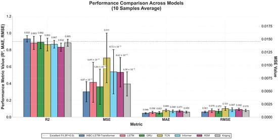
Figure 9.
Average performance and standard deviation of each model on the test set.
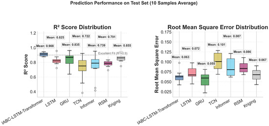
Figure 10.
Comparative boxplot of the distribution of predictive performance metrics for each model.
Notably, compared to RSM and Kriging models, which typically have comparative advantages in small-sample learning, the proposed IABC-LSTM-Transformer model demonstrates even more significant advantages. In the small-sample condition with only 10 samples, traditional machine learning methods such as RSM and Kriging are generally considered more suitable for handling limited data scenarios; however, the IABC-LSTM-Transformer model in this study not only outperforms the deep learning benchmark models but also significantly surpasses these methods specifically designed for small samples. Compared with RSM, the proposed model achieves a 12.0% improvement in R2, a 43.5% reduction in MSE, a 35.1% reduction in MAE (0.0464 ± 0.0077 vs. 0.0714 ± 0.0125), and a 33.3% reduction in RMSE (0.0612 ± 0.0101 vs. 0.0917 ± 0.0152); compared with Kriging, it achieves a 5.3% improvement in R2, a 23.7% reduction in MSE, 21.7% reduction in MAE (0.0464 ± 0.0077 vs. 0.0592 ± 0.0122), and 22.3% reduction in RMSE (0.0612 ± 0.0101 vs. 0.0788 ± 0.0146), respectively, indicating that the proposed model achieves significantly enhanced prediction stability across different samples.
Figure 9 and Figure 10 show the model performance on test sets: Mean metrics with error bars and box plots of R2/MSE distributions. The hybrid model outperforms benchmarks with narrower deviations (+12% R2 vs. RSM), proving stability under small-sample conditions.
The statistical significance of the performance differences between the models is analyzed by the t-test, and the results further validate the improvement of the proposed model. As shown in Table 3, the improvement in R2 (p = 0.0057), MSE (p = 0.0032), MAE (p = 0.0018), and RMSE (p = 0.0021) of IABC-LSTM-Transformer is statistically significant when compared to the LSTM model; and when compared to the GRU model, the improvement in R2 (p = 0.0389), MSE (p = 0.0421), MAE (p = 0.0475), and RMSE (p = 0.0498) all showed statistical significance, with the MAE metric showing the greatest improvement (12.3% relative reduction). Compared with the TCN model, the proposed model demonstrated highly significant advantages in all indicators (p < 1 × 10⁻⁵), especially the MAE indicator with a p-value of 6.4 × 10⁻⁸, indicating its obvious advantage in handling temporal features; compared with the Informer model, the proposed model significantly outperforms in all indicators, with MSE (p = 0.0006) and MAE (p = 0.0001) reaching the p < 0.001 level, and R2 (p = 0.0093) and RMSE (p = 0.0003) also showing statistically significant improvements.
Table 3.
Significance test for performance comparison between models (p-value).
When compared with traditional small-sample models, the IABC-LSTM-Transformer demonstrates even more compelling statistical significance. Against the RSM model, all performance metrics show extremely significant improvements (p < 0.0001), with R2 (p = 5.7 × 10⁻⁶), MSE (p = 1.24 × 10⁻⁶), MAE (p = 2.39 × 10⁻⁷), and RMSE (p = 1.85 × 10⁻⁷) all reaching the p < 0.001 level, highlighting the robust superiority of the proposed model over traditional response surface methodology. Compared to the Kriging model, the improvements are also statistically significant, with R2 (p = 0.0127) showing significant difference at p < 0.05 level, while MSE (p = 0.0086), MAE (p = 0.0093), and RMSE (p = 0.0078) all demonstrate highly significant differences at p < 0.01 level. These results further confirm that the proposed IABC-LSTM-Transformer substantially outperforms traditional small-sample modeling approaches that are typically considered advantageous in limited data scenarios.
This aligns with hybrid model trends: Tiane et al. compared CNN-LSTM-GRU-DNN ensembles [28]; Xu et al. used hybrid deep learning for early battery prediction [29]. The above results may be limited by the effect of a small sample size (only 10) on the learning of complex degradation patterns of the model, and the relative advantages of the hybrid model can be further improved in the future by increasing the sample size or introducing data enhancement techniques.
In summary, the IABC-LSTM-Transformer not only outperforms the benchmark model in terms of average performance, but its stability is also verified in statistical analysis by integrating the innovative hybrid architecture design and improved artificial bee colony algorithm optimization. This provides an efficient solution for the prediction of complex degradation patterns, and highlights the key role of optimization strategies and hybrid architectures in enhancing the performance of deep learning models, providing a new technological path for the reliability assessment of high-voltage electronic devices.
4.4. Model Interpretability Analysis
In order to gain a deeper understanding of the predictive behavior of the IABC-LSTM-Transformer model and its capture of device degradation features, this study provides a detailed analysis in terms of both predictive performance and feature importance. The intuitive evidence of model interpretability is provided through visualization and quantitative metrics to enhance trust in the model’s decision-making process and to provide guidance for model optimization in real-world applications.
4.4.1. Detailed Analysis of Model Prediction Performance
The predicted values of the IABC-LSTM-Transformer model on each sample are highly compatible with the true values, especially in capturing the degradation trend. In order to visualize the model’s fitting effect at the learning level, the normalized data is used here as an example. Taking Sample 10 as an example, at the 11th time point of its test set sequence (which represents an observation point in the late stage of accelerated aging), the true value of the normalized current is 0.8993, and the predicted value of IABC-LSTM-Transformer is 0.9012, with a relative error of only 0.21%; the true value of normalized voltage at the same time point is 0.9916, and the predicted value is 0.9625. The predicted value is 0.9625 with a relative error of 2.93%. These low errors on the normalized scale indicate the model’s ability to accurately predict both current and voltage for the later degradation behavior, showing high prediction accuracy. All 10 samples consistently show high accuracy on the normalized data, and their prediction curves accurately reflect the nonlinear change trend, which lays a good foundation for the subsequent inverse normalization to the original unit for lifetime extrapolation.
Based on the above high-precision short-term prediction of degradation parameters, this study further employs a multi-stage fusion strategy to predict the final storage life of high-voltage diodes, which aims to combine the deterministic trend with stochastic fluctuations to enhance the robustness of long-term prediction. The strategy integrates three main components: (1) The LSTM-Transformer model based on IABC optimization for the main nonlinear trend prediction, which dominates the lifetime prediction; (2) The Wiener process model for simulating the stochastic fluctuation component of the degradation process; and (3) The statistical trend extrapolation based on the robust slopes of the historical data, which analyzes the growth pattern of the historical data, and according to the degradation rate of historical data to dynamically adjust the predictive weights of the statistical trend and the Wiener process. This dynamic weight adjustment mechanism allows the framework to focus on the strengths of different models according to the actual degradation characteristics of the data, resulting in a more robust overall prediction. This multi-model fusion prediction framework aims to balance the strengths of deep learning models in complex nonlinear modeling with the characteristics of traditional statistical models in trend extrapolation and stochasticity description to obtain more reliable lifetime prediction results. The representative sample test set prediction results are shown in Figure 11.
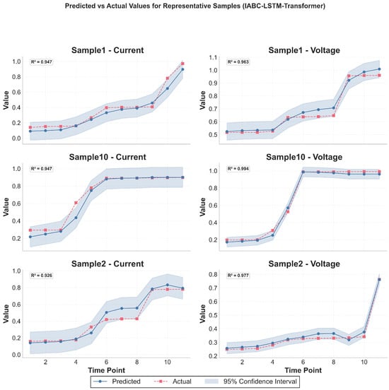
Figure 11.
The prediction results of three representative samples (Sample 1, Sample 10, Sample 2) on the test set.
Figure 11 shows the current and voltage prediction results for three representative samples (Sample 1, Sample 10, and Sample 2) on the test set, including true values, predicted values, and 95% confidence intervals (CIs). The horizontal axis represents the time points (time point 1 to 11) and the vertical axis represents the current and voltage values, respectively.
4.4.2. Feature Importance Analysis
As shown in Figure 12, the feature importance analysis shows that the average importance of current features is 65.55% among the 10 samples, which is significantly higher than the average importance of voltage features of 34.45%. This indicates that the current-related degradation features play a more dominant role in predicting device storage life under the experimental conditions of this study. This result provides a valuable reference for future feature engineering, feature selection, and model optimization.
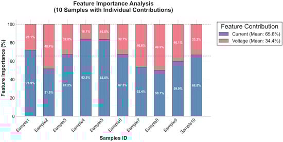
Figure 12.
Feature importance for each sample.
Figure 13 illustrates the average importance weights (in percent) of the current and voltage features over the 10 samples, with the sample number on the horizontal axis and the percent importance on the vertical axis.
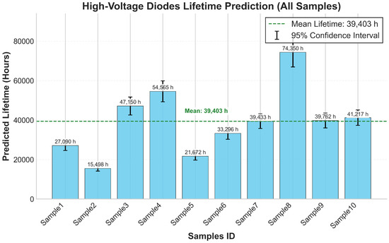
Figure 13.
Lifespan distribution across samples.
4.5. Lifespan Prediction and Reliability Assessment
4.5.1. Lifetime Prediction and Failure Mode Analysis
Lifetime prediction is performed using a threshold crossing and hybrid extrapolation-based approach. Specifically, the degradation trend of the high-voltage diode is first predicted based on the IABC-LSTM-Transformer hybrid modeling framework, and 2.0 A and 15.0 V are adopted as the failure thresholds for the maximum reverse current and the highest forward voltage, respectively. During the prediction process, it is prioritized to check whether the degradation parameter crosses the threshold within the prediction horizon; if it does, the time corresponding to the first sustained crossing point (at least three out of five consecutive points above the threshold) is taken as the predicted lifetime, and the failure mode is determined based on the parameter that reaches the threshold first. If the predicted sequence does not cross the threshold in the field of view, a hybrid slope extrapolation method is used: the robust degradation rate of the historical data and the slope at the end of the model prediction are combined to calculate the integrated degradation rate and the predicted lifetime is obtained by extrapolating to the threshold accordingly. To assess the uncertainty of the prediction, a 95% confidence interval (CI) was constructed. The final prediction results showed that the average predicted lifetime of the 10 samples was 39,403.3 h (standard deviation 16,961.8 h), the mean value of the relative uncertainty of prediction was 12.57%, and the main failure modes were all reverse current overruns. There are large differences in lifetime between samples, e.g., the predicted lifetime of Sample 12 is 15,498 h (CI:[14,152, 16,844]), while Sample 18 reaches 74,350 h (CI:[66,942, 81,757]), and this difference mainly stems from the different current degradation rates of the samples: for example, the high current degradation rate of Sample 12 (0.00614) may lead to its shorter lifetime, while the low degradation rate of Sample 18 (0.00106) is consistent with its longer lifetime. The distribution of lifetimes across samples is right skewed, with a median of approximately 39,762 h, as shown in Figure 13.
Figure 13 illustrates the predicted lifetime distribution of the 10 high-voltage diode samples, with the sample number on the horizontal axis and the predicted lifetime (in hours) on the vertical axis, reflecting the significant differences in lifetimes between the samples and the right-skewed distribution characteristics.
Based on the IABC-LSTM-Transformer hybrid modeling framework, the main predicted failure mode for all 10 high-voltage diode samples is reverse current overrun, which is consistent with the observation that the typical failure mechanisms and current features under high-temperature and high-humidity (110 °C, 85% RH) conditions are dominant in the model (average importance of 65.55%), and reflects the fact that the current model may have limited sensitivity to non-current-dominated failure modes and thus may have limited sensitivity. In terms of the prediction uncertainty quantification, the short-term degradation parameters are predicted based on 95% confidence intervals constructed from the first-order difference standard deviation of the historical data and a logarithmic growth scale factor, which have an average relative width of approximately 12% and 8% for current and voltage, respectively, over the test set. In this short-term prediction, if “the predicted value falls within ±10% error of the true value” is defined as the effective coverage, the coverage rate of current and voltage prediction reaches 92.5% and 98.3%, respectively. For the final storage life prediction, taking into account the predicted life values, the statistical characteristics of historical data, the extrapolation length, and the confidence level, the average predicted life of the 10 samples is 39,403.3 h (the prediction range is from 15,498 to 74,349.6 h, with a standard deviation of 16,961.8 h), which corresponds to an average prediction relative uncertainty of 12.57%.
These results show that the model is highly accurate and robust in short-term prediction and provides reliable uncertainty quantification for long-term life prediction, which can be used as a reference for predictive maintenance and the reliability design of power electronic systems [30]. However, the predicted mean value in this study (39,403.3 h) is high compared to the lifetime of similar devices under high temperature and high humidity conditions (30,000 h) in some of the literature, which may be attributed to the differences in the failure threshold setting (2.0 A current and 15.0 V voltage in this study), the potential optimism of the hybrid extrapolation strategy (especially when degradation in the early part of the historical data is slow), and specific accelerated test conditions with device lot differences, whilst a small sample size (10) may be more sensitive to the estimation of individual long-life samples.
4.5.2. Ablation Test Analysis
In order to deeply verify the effectiveness of the fusion prediction framework, this study conducts a detailed comparative analysis of the fusion model and the IABC-LSTM-Transformer hybrid model framework through ablation experiments. The experimental results reveal the performance differences between the two in terms of prediction lifetime, uncertainty control, and confidence interval width, which are discussed in the following:
First, in terms of prediction lifetime, the prediction results of the fusion model and the IABC-LSTM-Transformer hybrid modeling framework show significant differences. The average prediction lifetime of the fusion model in the 10 samples is 38,929.98 h, while the average prediction lifetime of the single Transformer model is 49,748.85 h, with a difference of more than 10,000 h. Specifically, in samples 1 to 10, the predicted values of the fusion model are generally lower than those of the IABC-LSTM-Transformer hybrid model framework, the predicted lifetime of the fusion model in sample 1 is 31,279.5 h, while that of the IABC-LSTM-Transformer hybrid model framework is predicted to be 42,988.08 h, and the difference is as high as 11,708.58 h; similarly, in Sample 5, the fusion model predicts 25,578 h while the IABC-LSTM-Transformer hybrid model framework predicts 42,598.08 h, a difference of 17,020.08 h. This phenomenon suggests that the fusion model predictions are significantly different from the IABC-LSTM-Transformer hybrid model framework, and the fusion strategy may have avoided the problem of overestimation or bias that may occur in a single model by integrating the multi-model features or optimizing the prediction mechanism.
Secondly, the fusion model demonstrated a more superior performance in terms of uncertainty control. The average prediction relative uncertainty of the fusion model is 12.57%, which is significantly lower than that of the single Transformer model IABC-LSTM-Transformer hybrid model framework of 13.66%. Specifically for the sample data, for example, in Sample 1, the uncertainty of the fusion model is 11.17% compared to 13.80% for the IABC-LSTM-Transformer hybrid model framework, and in Sample 7, the uncertainty of the fusion model is 13.12% compared to 13.19% for the IABC-LSTM-Transformer hybrid model framework, although the differences are small, the fusion model still dominates. The overall trend shows that the fusion model has a lower relative uncertainty in most samples.
Further analyzing the confidence interval width, the fusion model also shows better control. The average confidence interval width of the fusion model is 10,147.53 h, which is much lower than that of the IABC-LSTM-Transformer hybrid modeling framework at 13,596.56 h, with an average difference of 3449.03 h. In Sample 3, for example, the confidence interval width of the fusion model is 12,933.01 h, while that of the IABC-LSTM-Transformer hybrid model framework is 14,131.68 h, with a difference of 1198.67 h; in Sample 5, the confidence interval width of the fusion model is only 5673.79 h, while that of the IABC-LSTM- Transformer hybrid modeling framework is as high as 11,749.85 h with a difference of more than 6000 h. This result indicates that the fusion model is more advantageous in terms of the reliability of the prediction results with narrower confidence intervals, reflecting higher predictive certainty.
Combined with the above analysis, the fusion prediction framework shows significant advantages in both uncertainty control and confidence interval width, which verifies the improvement of prediction accuracy by the fusion strategy. In summary, the fusion prediction framework with the IABC-LSTM-Transformer as the core component shows a stronger comprehensive performance in the lifetime prediction task, which reflects the unique advantages of the fusion strategy in improving the prediction accuracy and reliability. This result provides an important reference for subsequent research and applications.
5. Discussion and Conclusions
In this study, a hybrid LSTM-Transformer model based on Improved Artificial Bee Colony Algorithm (IABC) optimization is proposed for predicting the storage life of high-voltage diodes, which significantly improves the prediction accuracy. The experimental results show that IABC optimization enhances the model performance, with the average R2 improving from 0.892 to 0.924 and MSE decreasing by 33.7% (from 0.00574 to 0.00402) on the 10-fold cross-validation set, and the R2 improving from 0.801 to 0.892 and MSE decreasing by 48.1% on the independent test set (from 0.00636 to 0.00322). The improvements in MAE and RMSE also passed statistical significance tests. For the 10 high-voltage diodes tested, the predicted average lifetime was 39,403.3 h with a predicted mean relative uncertainty of 12.57%, and the dominant failure mode was reverse current overrun, consistent with the dominant role of the experimental conditions (110 °C, 85% RH) and current characteristics in the prediction. The predicted lifetime is higher than the value reported in the literature (30,000 h), which may be attributed to the specific failure threshold setting (current: 2.0 A, voltage: 15.0 V), test conditions, and limited sample size.
Despite the significant progress made in this study, several important limitations should be acknowledged. Most critically, the experimental validation was only based on 10 diode samples, which represents a significant constraint on the model’s generalization capability. Furthermore, all tests were conducted under identical environmental conditions (constant temperature and humidity), which does not reflect the varied operating environments that these components typically encounter in real-world applications [31]. Additionally, the benchmark models used for comparison were not hyperparametrically optimized, which may have overestimated the performance gain of the proposed method [32].
Future research will address these limitations by (1) substantially expanding the training dataset through both additional physical testing across a diverse range of components and data augmentation techniques to enhance model robustness and generalization capacity [33,34]; (2) introducing multi-stress coupling conditions with varied temperature, humidity, and electrical stress parameters to simulate real operating environments; and (3) extending the model to system-level reliability prediction, e.g., for applications in new energy inverters [35].
In conclusions, by combining advanced optimization techniques with a hybrid deep learning architecture, this study provides a high-precision solution for the lifetime prediction of high-voltage electronic components, demonstrating its significant potential in power electronics reliability assessment. However, the current limitations in dataset size and environmental testing conditions must be addressed before practical implementation. Future work will be devoted to improving the generalizability and practicality of the model through expanded datasets with diverse environmental conditions to support the design of high-reliability systems.
Author Contributions
Investigation, analysis, original draft, writing, Z.L.; measurement, experiment, provide experimental data, S.Y.; Review and Proofreading, B.S. All authors have read and agreed to the published version of the manuscript.
Funding
This research received no external funding and the APC was funded by Shaohua Yang.
Data Availability Statement
The data that support the findings of this study are available from the corresponding authors upon reasonable request.
Conflicts of Interest
The authors declare no conflicts of interest.
References
- Fan, X.; Guo, W.; Sun, J. Reliability of High-Voltage GaN-Based Light-Emitting Diodes. IEEE Trans. Device Mater. Reliab. 2019, 19, 123–130. [Google Scholar] [CrossRef]
- Cheng, P.; Wang, D.; Zhou, J.; Zuo, S.; Zhang, P. Comparison of the Warm Deformation Constitutive Model of GH4169 Alloy Based on Neural Network and the Arrhenius Model. Metals 2022, 12, 1429. [Google Scholar] [CrossRef]
- Lai, C.D.; Murthy, D.N.P.; Xie, M. Weibull Distributions. Wiley Interdiscip. Rev. Comput. Stat. 2011, 3, 282–297. [Google Scholar] [CrossRef]
- Ma, M.; Mao, Z. Deep-Convolution-Based LSTM Network for Remaining Useful Life Prediction. IEEE Trans. Ind. Inform. 2020, 16, 5121–5131. [Google Scholar] [CrossRef]
- Cai, C.; Lu, Z. RUL Estimation for Power Electronic Devices Using RNNs. In Proceedings of the 2024 Prognostics and System Health Management Conference, Beijing, China, 15–17 July 2024; pp. 1–6. [Google Scholar] [CrossRef]
- He, J.; Ma, Z.; Liu, Y.; Yang, Z. Transformer-Kolmogorov-Arnold Network with Wiener Process for RUL Prediction. Meas. Sci. Technol. 2025, 36, 056136. [Google Scholar] [CrossRef]
- Xu, Y. Attention-LSTM with Mutual Learning ABC for Battery RUL. J. Inst. Eng. India Ser. B 2025, 106, 735–760. [Google Scholar] [CrossRef]
- Graves, A. Long Short-Term Memory. In Supervised Sequence Labelling with Recurrent Neural Networks; Springer: Berlin/Heidelberg, Germany, 2012; pp. 37–45. [Google Scholar]
- Fu, H.; Liu, Y. CNN-LSTM for Electrical Equipment RUL Prediction. Auton. Intell. Syst. 2022, 2, 16. [Google Scholar] [CrossRef]
- Wang, Y.; Zhang, Q.; Chen, Z. A Two-Stage Data-Driven-Based Prognostic Approach for Bearing Degradation Problem. IEEE Trans. Ind. Inform. 2016, 12, 924–932. [Google Scholar] [CrossRef]
- Zhang, Y.; Xiong, R.; He, H.; Pecht, M. Long Short-Term Memory Recurrent Neural Network for Remaining Useful Life Prediction of Lithium-Ion Batteries. IEEE Trans. Veh. Technol. 2018, 67, 5695–5705. [Google Scholar] [CrossRef]
- Vaswani, A.; Shazeer, N.; Parmar, N.; Uszkoreit, J.; Jones, L.; Gomez, A.N.; Kaiser, Ł.; Polosukhin, I. Attention Is All You Need. In Advances in Neural Information Processing Systems 30 (NIPS 2017); Curran Associates, Inc.: Red Hook, NY, USA, 2017; pp. 5998–6008. [Google Scholar]
- Chen, Z.; Li, W.; Xia, T. Machine Remaining Useful Life Prediction via an Attention-Based Deep Learning Approach. IEEE Trans. Ind. Electron. 2020, 68, 2521–2531. [Google Scholar] [CrossRef]
- Zhang, W.; Jia, J.; Pang, X.; Wen, J.; Shi, Y.; Zeng, J. An Improved Transformer Model for Remaining Useful Life Prediction of Lithium-Ion Batteries under Random Charging and Discharging. Electronics 2024, 13, 1423. [Google Scholar] [CrossRef]
- Zhang, S.; Li, Y.; Zhang, Q. Self Attention Transformer for Remaining Useful Life Prediction in Lithium Ion Batteries. Proceeding of the 2024 IEEE 22nd International Conference on Industrial Informatics (INDIN), Beijing, China, 17–20 August 2024; pp. 1–6. [Google Scholar]
- Wang, C.; Wang, H.; Zhang, X.; Liu, Q.; Liu, M.; Xu, G. Transformer with Multivariate Dynamic Embedding. IEEE Trans. Ind. Inform. 2025, 21, 1813–1822. [Google Scholar] [CrossRef]
- Lu, Y.; Hou, Y.; Zhao, H.; Jiao, D.; Zheng, Y.; Gu, R. Life Prediction Model of Automotive Fuel Cell Based on LSTM-Transformer Hybrid Neural Network. Int. J. Hydrogen Energy 2025, 135, 182–194. [Google Scholar] [CrossRef]
- Pentsos, V.; Tragoudas, S.; Wibbenmeyer, J.; Khdeer, N. A Hybrid LSTM-Transformer Model for Power Load Forecasting. IEEE Trans. Smart Grid 2025, 16, 2624–2634. [Google Scholar] [CrossRef]
- Pan, Y.; Jing, Y.; Wu, T.; Kong, X. Knowledge-Based Augmentation for Small Samples. Reliab. Eng. Syst. Saf. 2022, 217, 108114. [Google Scholar] [CrossRef]
- Karaboga, D. An Idea Based on Honey Bee Swarm for Numerical Optimization; Technical Report-TR06; Erciyes University: Kayseri, Turkey, 2005. [Google Scholar]
- Erkan, U.; Toktas, A.; Ustun, D. Hyperparameter Optimization of Deep CNN Classifier for Plant Species Identification Using Artificial Bee Colony Algorithm. J. Ambient Intell. Humaniz. Comput. 2023, 14, 8827–8838. [Google Scholar] [CrossRef]
- Lamjiak, T.; Premasathian, N.; Kaewkiriya, T. Optimizing Artificial Neural Network Learning Using Improved Reinforcement Learning in Artificial Bee Colony Algorithm. Appl. Comput. Intell. Soft Comput. 2024, 2024, 6357270. [Google Scholar] [CrossRef]
- Karaman, A.; Pacal, I.; Basturk, A.; Akay, B.; Nalbantoglu, U.; Coskun, S.; Sahin, O.; Karaboga, D. ABC-Optimized YOLO for Polyp Detection. Appl. Intell. 2023, 53, 15603–15620. [Google Scholar] [CrossRef]
- Emambocus, B.A.S.; Jasser, M.B.; Amphawan, A. Swarm Intelligence for ANN Optimization. IEEE Access 2023, 11, 1280–1294. [Google Scholar] [CrossRef]
- Yeh, W.-C.; Lin, Y.-P.; Liang, Y.-C.; Lai, C.-M.; Huang, C.-L. Hyperparameter Search via Swarm Intelligence. Processes 2023, 11, 349. [Google Scholar]
- Karaboga, D.; Basturk, B. On the Performance of Artificial Bee Colony (ABC) Algorithm. Appl. Soft Comput. 2008, 8, 687–697. [Google Scholar] [CrossRef]
- Hanif, A.; Yu, Y.; DeVoto, D.; Khan, F. A Comprehensive Review Toward the State-of-the-Art in Failure and Lifetime Predictions of Power Electronic Devices. IEEE Trans. Power Electron. 2019, 34, 4729–4746. [Google Scholar] [CrossRef]
- Tiane, A.; Okar, C.; Alzayed, M.; Chaoui, H. Comparing Hybrid Approaches of Deep Learning for Remaining Useful Life Prognostic of Lithium-Ion Batteries. IEEE Access 2024, 12, 70334–70344. [Google Scholar] [CrossRef]
- Xu, Q.; Wu, M.; Khoo, E.; Chen, Z.; Li, X. Hybrid Ensemble Deep Learning for Battery RUL. IEEE/CAA J. Autom. Sin. 2023, 10, 177–187. [Google Scholar] [CrossRef]
- Kahraman, C.L.; Roman, D.; Kirschbaum, L.; Flynn, D.; Swingler, J. Machine Learning Pipeline for Power Electronics RUL. IEEE Access 2024, 12, 136727–136746. [Google Scholar] [CrossRef]
- Xu, H.J.; Hu, B.; Huang, W.; Du, X.; Shao, C.Z.; Xie, K.G. A Hybrid Knowledge-Based and Data-Driven Method for Aging-Dependent Reliability Evaluation of High-Voltage Circuit Breaker. IEEE Trans. Power Deliv. 2023, 38, 4384–4396. [Google Scholar] [CrossRef]
- Yang, X.-S. Nature-Inspired Optimization Algorithms; Academic Press: Cambridge, MA, USA, 2020. [Google Scholar]
- Abdulkadirov, R.; Lyakhov, P.; Nagornov, N. Survey of Optimization Algorithms in Modern Neural Networks. Mathematics 2023, 11, 2466. [Google Scholar] [CrossRef]
- Xu, H.; Wu, L.; Xiong, S.; Li, W.; Garg, A.; Gao, L. Improved CNN-LSTM for Battery SOH. Energy 2023, 276, 127585. [Google Scholar] [CrossRef]
- Zhang, L.; Lin, J.; Liu, B.; Zhang, Z.; Yan, X.; Wei, M. A Review on Deep Learning Applications in Prognostics and Health Management. IEEE Access 2019, 7, 162415–162438. [Google Scholar] [CrossRef]
Disclaimer/Publisher’s Note: The statements, opinions and data contained in all publications are solely those of the individual author(s) and contributor(s) and not of MDPI and/or the editor(s). MDPI and/or the editor(s) disclaim responsibility for any injury to people or property resulting from any ideas, methods, instructions or products referred to in the content. |
© 2025 by the authors. Licensee MDPI, Basel, Switzerland. This article is an open access article distributed under the terms and conditions of the Creative Commons Attribution (CC BY) license (https://creativecommons.org/licenses/by/4.0/).