Research on Coordinated Planning and Operational Strategies for Novel FACTS Devices Based on Interline Power Flow Control

Abstract

Under the “dual carbon” goals and rapid clean energy development, power grids face challenges including rapid load growth, uneven power flow distribution, and limited transmission capacity. This paper proposes a novel FACTS device with fault tolerance and switchable topology that maintains power flow control over multiple lines during N-1 faults, enhancing grid safety and economy. The paper establishes a steady-state mathematical model based on additional virtual nodes and provides power flow calculation methods to accurately reflect the device’s control characteristics. An entropy-weighted TOPSIS method was employed to establish a quantitative evaluation system for assessing the grid performance improvement after FACTS device integration. To address interaction issues among multiple flexible devices, an optimization planning model considering th3e coordinated effects of UPFC and VSC-HVDC was constructed. Multi-objective particle swarm optimization obtained Pareto solution sets, combined with the evaluation system, to determine the optimal configuration schemes. Considering wind power uncertainty and fault risks, we propose a system-level coordinated operation strategy. This strategy constructs probabilistic risk indicators and introduces topology switching control constraints. Using particle swarm optimization, it achieves a balance between safety and economic objectives. Simulation results in the Jiangsu power grid scenarios demonstrated significant advantages in enhancing the transmission capacity, optimizing the power flow distribution, and ensuring system security.

1. Introduction

With the rapid growth of renewable energy installations and increasing cross-regional power transmission demands, modern power systems face severe challenges in power flow regulation, voltage stability, and operational flexibility. The International Energy Agency predicts that renewable energy will account for 42% of global electricity supply by 2029 [1]. The role of power electronic converters in modern distribution systems has become increasingly important, with their evolution, current challenges, and future trends warranting in-depth study [2].

Impact assessments of high penetration renewable energy and electric vehicles on distribution network operation revealed that traditional distribution networks face unprecedented challenges [3], thus reliability evaluations of active distribution networks with multiple renewable energy sources have become a critical technical issue [4]. Against this backdrop, flexible AC transmission system (FACTS) technology has attracted widespread attention as a key solution for improving transmission performance and enhancing system stability [5]. In terms of FACTS device optimization control, Chen et al. proposed a coordinated control method for UPFC for power flow optimization and power quality enhancement [6]. Wang et al. further studied multi-objective optimization methods for UPFC controllers in distribution networks [7]. For offshore wind power systems, Tang et al. proposed harmonic mitigation methods and control strategies based on distributed power flow controllers [8]. Multi-device coordinated control technology has also undergone significant development. Zhao et al. studied distributed coordination control strategies for multiple STATCOMs in distribution networks [9]. In low-voltage distribution systems, Yang et al. proposed a novel control strategy for soft open points to address terminal voltage violations and load rate imbalance [10]. Regarding distribution network fault recovery technology, Jian et al. studied supply restoration strategies for data centers in flexible distribution networks [11]. Hu et al. proposed an island fault recovery method for distribution networks based on flexible interconnection devices with energy storage [12]. Xu et al. further proposed an optimal power restoration strategy for multi-terminal flexible interconnected distribution networks based on flexible interconnection devices and network reconfiguration [13]. For operational optimization of flexible interconnected distribution networks, Zhao et al. studied fault recovery strategies for flexible interconnected distribution networks with SOP flexible closed-loop operation [14]. Zhang et al. analyzed solutions for load transfer without power interruption in distribution lines with a 30° phase angle difference [15], while Zhou et al. constructed a power transfer optimization model for active distribution networks considering loop closing current constraints [16]. In fault location technology, Chen et al. applied distributed positioning technology to distribution network fault location [17]. Xu et al. analyzed fault characteristics of distribution networks with PST loop closing devices under small current grounding systems [18]. The application of advanced control technologies continues to develop. Liu et al. studied advanced control strategies for MMC-STATCOM under unbalanced grid conditions [19]. Tang et al. researched topology and control methods for uninterrupted ice melting devices based on non-contact coupling power flow controllers [20]. Li et al. proposed a deep reinforcement learning-based intelligent dynamic voltage restorer for voltage sag compensation [21]. In terms of equipment performance optimization, Yang et al. studied hybrid energy storage-based dynamic voltage restorers, achieving cost reduction and performance enhancement [22]. Liu et al. proposed adaptive group control strategies for distributed static series compensators [23]. Zhao et al. proposed hierarchical control strategies for cascaded STATCOM systems for power quality improvement [24]. Tang et al. also studied harmonic current rates for the exchanged energy of unified distributed power flow controllers [25]. However, existing research exhibits three critical limitations: (1) most FACTS devices employ fixed topological structures, lacking effective fault tolerance during N-1 contingencies; (2) current control strategies inadequately address multi-device coordination issues, hindering system-level performance optimization; and (3) traditional planning methods often neglect operational risks and renewable energy uncertainties, limiting the adaptability to complex operational scenarios. To address these challenges, this paper proposes a topology-switching FACTS device based on interline power flow control. The device features multiple redundant operation modes, enabling rapid topology reconfiguration during faults to maintain continuous power flow regulation. A unified power flow model for topology-variable conditions was established, accompanied by multi-objective optimization strategies.

The main contributions of this paper include the following: (1) proposing a novel fault-tolerant FACTS topology with adaptive reconfiguration capabilities; (2) establishing a unified power flow analysis framework for topology-variable conditions; (3) constructing a multi-dimensional evaluation system integrating stability and economic indicators; and (4) proposing a system-level coordinated optimization strategy considering operational uncertainties.

The remainder of this paper is organized as follows. Section 2 details the proposed FACTS device topology and establishes its steady-state mathematical model. Section 3 develops a quantitative evaluation system and constructs the planning optimization framework. Section 4 designs the coordinated operation strategy considering uncertainty. Section 5 validates the methods through simulation analysis. Finally, Section 6 concludes with the research findings and future directions.

2. Topology and Steady-State Modeling of Novel FACTS Devices

2.1. Topological Configuration of Novel FACTS Devices

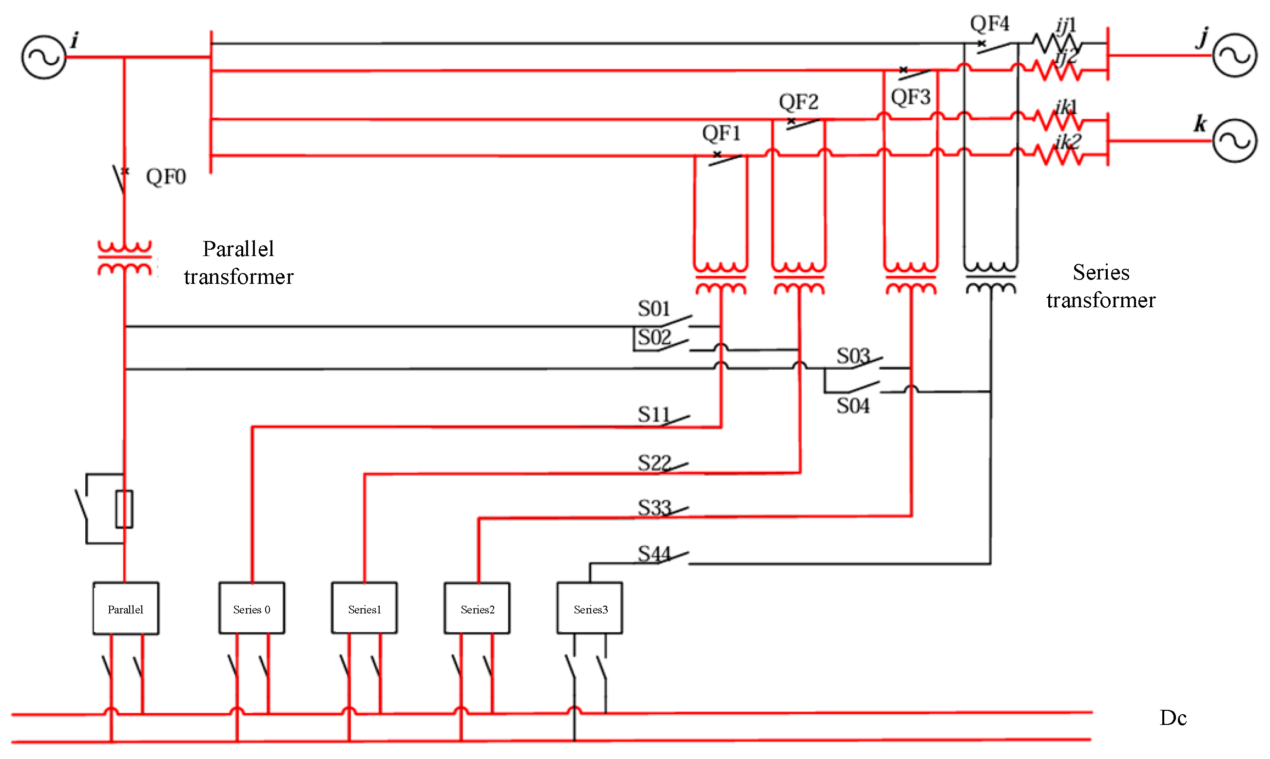
In order to cope with the uneven current distribution, fault tolerance, and economic requirements of multiple lines in the power grid, this paper proposes a new type of FACTS device based on inter-line current control. The device is improved on the basis of the traditional UPFC and IPFC topology, adopts a double circuit structure, and realizes the independent regulation of the active and reactive power of transmission lines through the synergistic action of series side and shunt side converter, and at the same time realizes the function of the standby path through the internal changeover switch. Figure 1 shows the basic topology of the new FACTS device.

In the proposed topology, four series-connected converters are employed to inject controllable sinusoidal voltages into the regulated transmission lines. These converters generate adjustable output voltages with independently regulated magnitudes and phase angles, enabling precise control of both active and reactive power flows in the lines. The shunt-connected converter primarily stabilizes the voltage of the common AC bus and compensates for potential voltage fluctuations caused by the series converters by absorbing or injecting reactive power. Each converter is equipped with transfer switches, allowing for rapid reconfiguration to redundant topologies during contingencies (e.g., converter or line failures) or under special operating conditions. This design not only reduces the hardware redundancy and engineering costs, but also demonstrates significant advantages in system security, flexibility, and economic efficiency.

2.2. Topology-Switching Principle

A core innovation of the novel FACTS device lies in its flexible topology-switching capability. During actual grid operation, controlled transmission lines or internal converters may fail due to faults, overloads, or other contingencies. Without timely adjustments, such failures could trigger voltage fluctuations and an uneven power flow distribution. In severe cases, they may even cause cascading system failures. To address these challenges, this study proposes a transfer switch-based topology-switching scheme, enabling the device to rapidly reconfigure to a redundant topology configuration during N-1 contingencies, thereby ensuring continuous stable operation of the system.

Figure 2 illustrates the topology-switching principle. In the diagram, when a fault occurs in a controlled transmission line (e.g., an anomaly in line ij), the converter on the faulty line is immediately isolated, and the transfer switch automatically disconnects the faulty branch, enabling the system to transition to the standby GIPFC mode. In cases of internal converter failure, the system switches to the dual-circuit IPFC mode by connecting a backup converter to the faulty branch. This process requires no manual intervention and completes within milliseconds, ensuring uninterrupted power flow regulation during faults. The figure demonstrates how transfer switches isolate and reconfigure internal units of the device during line or converter failures, achieving seamless redundant topology switching.

To characterize the post-switching adjustments in line parameters and power redistribution, this paper introduces the following correction formula. Assuming the conductance (Gij) and susceptance (Bij) of the controlled line ij change by ΔGij and ΔBij after a fault, the power adjustment is derived from the line power flow equation as:

$$\Delta P_{ij}^{dyn}=V_i{V}_j\left(\Delta G_{ij}\cos {\theta }_{ij}+\Delta B_{ij}\sin {\theta }_{ij}\right)$$

(1)

Equation (1) quantitatively describes the transient power redistribution caused by line parameter variations during switching operations. As illustrated in Figure 2, this dynamic adjustment ensures power flow balance within milliseconds after fault isolation.

Real-time switching control is implemented through a three-layer architecture:

(1) Fault detection layer

A high-speed digital signal processor (DSP) with a 10 kHz sampling rate continuously monitors the line currents, voltages, and converter status. The fault detection algorithm integrates differential protection and impedance detection principles, with its core criterion defined as:

$$I_{line}\left(t\right)-I_{line}\left(t-\Delta t\right)>K_{diff}\times I_{rated}$$

(2)

where the differential sensitivity factor is K_diff = 0.1 and sampling interval is Δt = 100 μs. This design enables the precise capture of microsecond-level fault current transients.

(2) Decision-making layer

A fuzzy logic-based decision system generates optimal switching strategies within 2~5 ms. The evaluation matrix covers four critical dimensions:

• Fault characteristics (type and location);
• System load status (real-time load ratio);
• Redundant path availability (topological connectivity analysis);
• Stability benefits (damping ratio improvement during transients).

Through multi-objective trade-offs, it dynamically selects the switching path with minimal system impact.

(3) Execution layer

Switching commands are executed via high-speed optical fiber links with a latency below 1 ms. A dual-channel redundant communication protocol ensures reliability:

• Primary channel: GOOSE messages based on IEC 61850-1-2013 (critical commands);
• Secondary channel: Modbus TCP (status monitoring and parameter configuration);

The complete process from fault detection to switching operation is strictly controlled within 10 ms, meeting the transient stability boundary requirements for power systems. The stable boundary adjustment is shown in

Table 1. Sampling rate specifications.

Monitoring Target	Rate
Voltage/current measurement	10 kHz
Converter status	1 kHz
Temperature and auxiliaries	100 Hz

.

This architecture ensures reliable topology switching (Figure 2) with millisecond-level precision.

Furthermore, to synchronize converter state adjustments during switching, the device implements coordinated control strategies including fault detection, switching execution, and control parameter updates. These processes are embedded into the iterative steady-state model-solving procedure, enabling smooth transitions between pre-fault and post-fault system states.

Overall, the topology-switching principle achieves fault-tolerant control under N-1 contingencies through rapid fault isolation, automatic redundant topology activation, and dynamic power redistribution. This mechanism provides robust protection for secure grid operation.

2.3. Steady-State Mathematical Model

To accurately characterize the power flow regulation effects of the novel FACTS device under different topology modes, this paper developed a steady-state mathematical model based on the additional virtual node method. This model equivalently represents the converter’s regulation capability as a synchronous voltage source. By introducing virtual nodes, the control voltage injected by the converters is converted into node power injections, forming a hybrid system integrated with traditional power flow calculation models. Key formulas and detailed derivations are provided below.

First, for any node i in the grid, the power injections are calculated using the conventional power flow equations:

$$P_i=V_i\sum _{j\in N}{V}_j\left(G_{ij}\cos {\theta }_{ij}+B_{ij}\sin {\theta }_{ij}\right)$$

(3)

$$Q_i=V_i\sum _{j\in N}{V}_j\left(G_{ij}\sin {\theta }_{ij}-B_{ij}\cos {\theta }_{ij}\right)$$

(4)

where Vi is the voltage magnitude at node i, ${\theta }_{ij}={\theta }_i-{\theta }_j$ is the phase angle difference, and Gij/Bij are the equivalent conductance/susceptance of the line. Equations (3) and (4) form the basis of grid-wide power balance.

To incorporate the novel FACTS device into power flow calculations, an additional virtual node h is introduced to represent the converter’s injected voltage and current. The power injection model for the virtual node is defined as:

$$P_h=V_h{I}_h\cos {\theta }_h,Q_h=V_h{I}_h\sin {\theta }_h$$

(5)

where Vh and Ih are the voltage and injected current at the virtual node, respectively, and θh is its phase angle. This equation integrates the converter’s regulation effects into the node power flow calculations.

For multi-converter systems, the active power conservation condition must be satisfied to ensure internal power balance:

$$\sum _{k=1}^{N_c}{P}_k^{\mathrm{inj}}=0$$

(6)

where Nc is the total number of converters in the device, and $P_k^{inj}$ is the active power injected by the k-th converter. Equation (6) guarantees power balance across the DC bus.

The output voltage of the series-side converter is decomposed into orthogonal components:

$$V_{se,x}=V_{se}\cos {\theta }_{se},V_{se,y}=V_{se}\sin {\theta }_{se}$$

(7)

where Vse is the magnitude of the series converter’s output voltage, and θse is its phase angle. This decomposition facilitates the independent analysis of active and reactive power contributions to the power flow.

During iterative solving, the Newton–Raphson method updates the converter’s power injections. Let $P_h^{(k)}$ and $Q_h^{(k)}$ denote the active and reactive power injections at the k-th iteration. The update formulas are:

$$P_h^{(k+1)}=P_h^{(k)}+\Delta P_h,Q_h^{(k+1)}=Q_h^{(k)}+\Delta Q_h$$

(8)

where ΔPh and ΔQh are power corrections derived from the Jacobian matrix. Equation (16) dynamically adjusts the converter’s power injections to approach predefined targets.

The shunt-side converter primarily regulates reactive power to maintain the voltage at the common node within a specified range:

$$V_i^{\min }\le V_i\le V_i^{\max }$$

(9)

Equation (9) imposes voltage stability constraints, preventing excessive fluctuations during converter adjustments.

During topology switching, the line parameters may change. The steady-state equivalent of dynamic adjustment (Equation (1)) is embedded in power flow constraints as:

$$\Delta P_{ij}^{ss}=V_i{V}_j\left(\Delta G_{ij}\cos {\theta }_{ij}+\Delta B_{ij}\sin {\theta }_{ij}\right)$$

(10)

where ΔGij and ΔBij represent post-switching changes in line conductance and susceptance, respectively, and $\Delta P_{ij}^{ss}$ quantifies the active power adjustment. This formula provides a basis for post-switching power redistribution.

Equation (1) describes the dynamic power redistribution during switching transients, while Equation (10) represents its integration into steady-state constraints. The mathematical equivalence ($\Delta P_{ij}^{dyn}=\Delta P_{ij}^{ss}$) validates the consistency between dynamic behavior and static operation models.

Finally, the global power balance condition must hold for steady-state operation:

$$\sum _{i\in N}\left(P_i+\sum _{h\in H}{P}_h\right)=0,\sum _{i\in N}\left(Q_i+\sum _{h\in H}{Q}_h\right)=0$$

(11)

Equation (11) serves as the fundamental boundary condition for power flow calculations, ensuring system-wide active and reactive power balance.

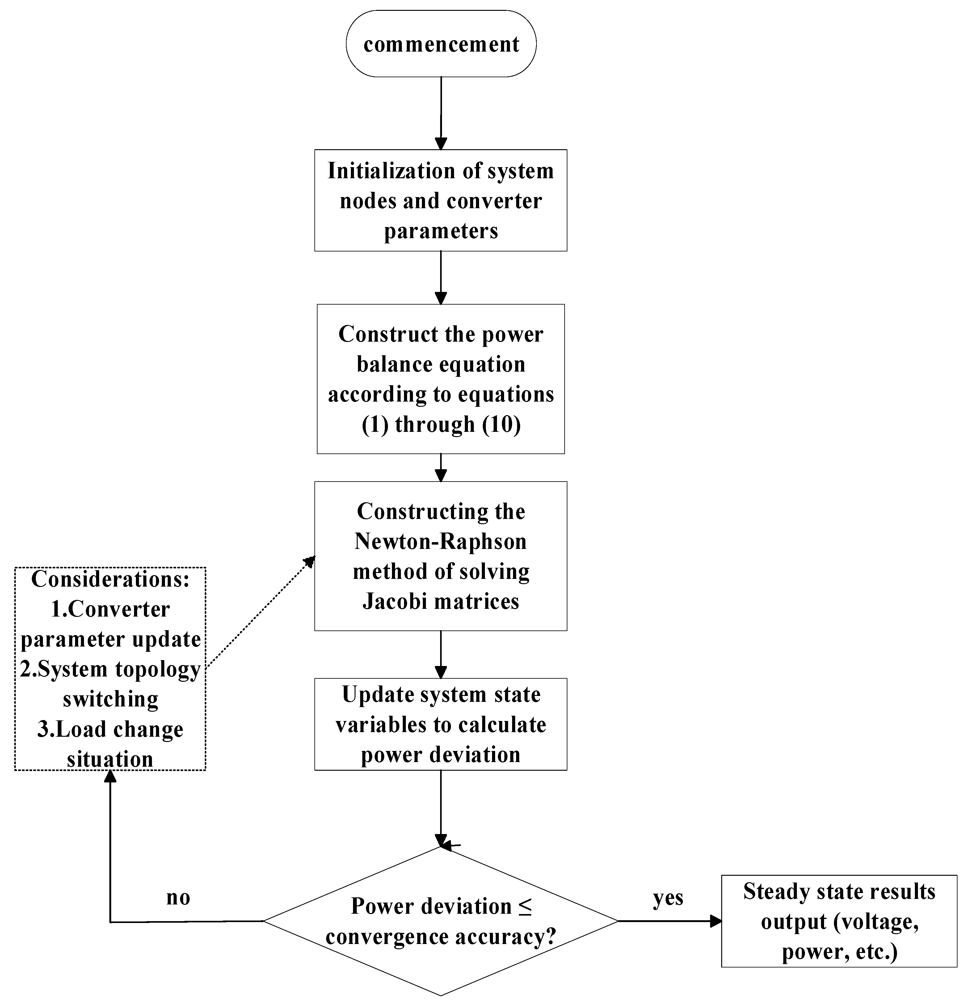
Figure 3 illustrates the solution flowchart for the steady-state model based on virtual nodes.

3. Quantitative Evaluation and Planning Optimization

3.1. Quantitative Evaluation Indicator System

To comprehensively evaluate the performance enhancement of power grids with FACTS devices, a multi-criteria evaluation system was established. The evaluation indicators were categorized into three groups: static stability indicators, dynamic security indicators, and economic efficiency indicators.

(1) Static stability indicators

Static stability reflects the grid’s ability to resist disturbances under steady-state conditions, focusing on node voltage fluctuations, power transmission capacity, and voltage margins. Key indicators include:

Voltage stability margin (Vmargin)

This metric quantifies the safety margin between the actual node voltage and predefined limits:

$$V_{margin}=\min \left\{{\displaystyle \frac{V_i-V_i^{\min }}{V_i^{\mathrm{nom}}}},{\displaystyle \frac{V_i^{\max }-V_i}{V_i^{\mathrm{nom}}}}\right\},i\in N$$

(12)

where Vi is the actual voltage at node i, Vimin and Vimax are the predefined minimum and maximum voltage thresholds, respectively, and Vinom is the rated voltage. This indicator reflects the system’s ability to maintain safe operation under disturbances.

Line transmission capacity (Ptrans)

This measures the improvement in power transfer capability of critical transmission lines after FACTS installation:

$$P_{trans}={\displaystyle \frac{P_{trans}^{\mathrm{new}}-P_{trans}^{\mathrm{old}}}{P_{trans}^{\mathrm{old}}}}\ast 100\%$$

(13)

where $P_{trars}^{old}$ and $P_{trars}^{new}$ represent the rated transmission capacities before and after FACTS deployment.

(2) Dynamic security indicators

Dynamic security evaluates the system’s transient recovery capability under disturbances (e.g., faults, load surges, or renewable energy fluctuations). Key indicators include:

Phase angle deviation (Δθ)

Defined as the maximum phase angle difference between critical nodes after a fault:

$$\Delta \theta =\underset{i,j\in N}{\max }|{\theta }_i-{\theta }_j|$$

(14)

where θi and θj are the voltage phase angles at nodes i and j, respectively. A smaller Δθ indicates better synchronization and dynamic stability.

Transient stability margin (T_margin)

Evaluates transient recovery capability using energy functions or time-domain simulations:

$$T_{margin}={\displaystyle \frac{E_{cr}}{E_{act}}}$$

(15)

where Ecr is the critical energy required for post-fault stabilization, and Eact is the actual energy released by the system. A higher Tmargin implies faster recovery.

(3) Economic efficiency indicators

These assess the trade-off between FACTS investment/operational costs and benefits such as improved transmission capacity and reduced losses. Key indicators include:

Investment economy (Cinv)

Represents the investment cost per unit capacity:

$$C_{inv}={\displaystyle \frac{C_{\mathrm{total}}}{S_{\mathrm{cap}}}}$$

(16)

where Ctotal is the total investment cost and Scap is the installed capacity.

Operational economy (Coper)

Combines maintenance, energy loss, and dispatch costs:

$$C_{oper}=\alpha \cdot C_{\mathrm{loss}}+\beta \cdot C_{\mathrm{maint}}$$

(17)

where Closs is the energy loss cost, Cmaint is the maintenance cost, and α, β are weighting coefficients.

A comprehensive evaluation function (Ftotal) integrates the normalized scores of the static, dynamic, and economic indicators:

$$F_{total}=w_1\cdot f_{static}+w_2\cdot f_{dynamic}+w_3\cdot f_{economic}$$

(18)

In Equation (18), fstatic, fdynamic, and feconomic represent the normalized comprehensive scores of the static, dynamic, and economic indicators, respectively, while w1, w2, and w3 denote their corresponding weights. This formula provides a quantitative basis for ranking planning alternatives and guiding optimization.

3.2. Quantitative Evaluation Methodology

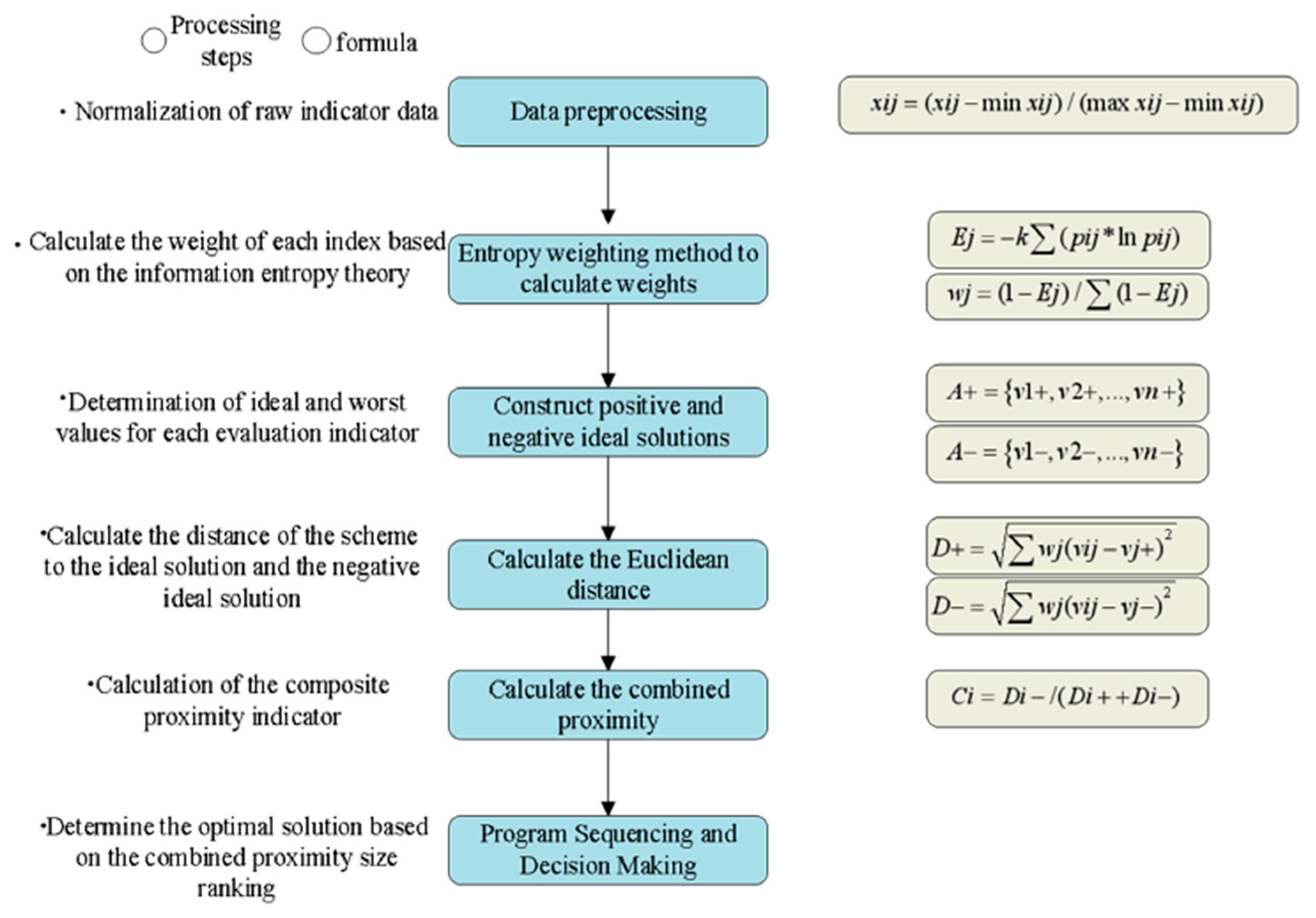
To synthesize multi-dimensional indicators for evaluating planning alternatives, this study employed the entropy weight method combined with the TOPSIS (Technique for Order Preference by Similarity to an Ideal Solution) approach. The TOPSIS method was selected for its effectiveness in ranking alternatives based on their geometric distance from both positive and negative ideal solutions, providing a clear and intuitive quantitative evaluation suited to the multi-dimensional nature of the established indicator system.

The entropy weight method objectively assigns weights to indicators based on their data dispersion. For m alternatives and n indicators, the normalized value yij of the j-th indicator for the i-th alternative is calculated as:

$$y_{ij}={\displaystyle \frac{x_{ij}-\min \left\{x_j\right\}}{\max \left\{x_j\right\}-\min \left\{x_j\right\}}},i=1,\dots ,m$$

(19)

Subsequently, the information entropy Ej for each indicator is derived:

$$E_j=-k\sum _{i=1}^m{y}_{ij}\ln (y_{ij}+\epsilon ),k={\displaystyle \frac{1}{\ln m}}$$

(20)

where ε is a small positive constant (set to 10⁻⁶) to avoid the undefined problem of the ln function when y_ij = 0. The weight wj of the j-th indicator is then determined as:

$$w_j={\displaystyle \frac{1-E_j}{{\displaystyle \sum _{j=1}^n}(1-E_j)}}$$

(21)

Following the entropy weight calculation, the TOPSIS method evaluates alternatives by measuring their proximity to ideal solutions. The positive ideal solution (A+) and negative ideal solution (A−) are defined as:

$$A^{+}=\{\max (y_{ij})\},A^{-}=\{\min (y_{ij})\},j=1,\dots ,n$$

(22)

The Euclidean distances from each alternative to A+ and A− are computed as:

$$D_i^{+}=\sqrt{\sum _{j=1}^n{w}_j{(y_{ij}-A_j^{+})}^2},D_i^{-}=\sqrt{\sum _{j=1}^n{w}_j{(y_{ij}-A_j^{-})}^2}$$

(23)

The relative closeness Ci, which quantifies the overall performance of each alternative, is given by:

$$C_i={\displaystyle \frac{D_i^{-}}{D_i^{+}+D_i^{-}}},0\le C_i\le 1$$

(24)

A higher Ci indicates superior performance across static, dynamic, and economic dimensions. This method provides a quantitative basis for ranking alternatives and guiding optimization decisions.

The quantitative evaluation process is illustrated in Figure 4, which details the complete workflow from raw indicator normalization, entropy weight calculation, and the construction of positive/negative ideal solutions to distance measurement and comprehensive score derivation.

To validate the robustness of the evaluation framework, four normalization approaches were compared:

Method definitions:

(1)

Vector normalization (Euclidean)

$$y_{ij}^{vector}={\displaystyle \frac{x_{ij}}{\sqrt{{\sum }_{i=1}^m{x}_{ij}^2}}}$$

(25)

(2)

Manhattan normalization (L1)

$$y_{ij}^{manhattan}={\displaystyle \frac{x_{ij}}{{\sum }_{i=1}^m\left|x_{ij}\right|}}$$

(26)

(3)

Max-min normalization (current)

$$y_{ij}^{maxmin}={\displaystyle \frac{x_{ij}-min\left\{x_j\right\}}{max\left\{x_j\right\}-min\left\{x_j\right\}}}$$

(27)

(4)

Z-score normalization

$$y_{ij}^{zscore}={\displaystyle \frac{x_{ij}-{\mu }_j}{{\sigma }_j}}$$

(28)

Comparative results:

Normalization Method	Ranking Correlation (Spearman’s ρ)	Computational Time (ms)	Ranking Stability
Max-Min (Original)	1.000	12.3	Baseline
Vector (Euclidean)	0.892	8.7	High
Manhattan (L1)	0.847	9.1	Moderate
Z-Score	0.923	11.8	High

Key findings:

(1) Ranking consistency: All normalization methods produced consistent top-tier rankings (ρ > 0.84), indicating the robustness of our evaluation framework.

(2) Computational efficiency: Vector normalization offered the fastest computation (8.7 ms vs. 12.3 ms for max-min), making it suitable for real-time applications.

(3) Stability analysis: Z-score normalization showed the highest stability under data perturbations (±5% parameter variation), while Manhattan normalization was the most sensitive to outliers.

3.3. Planning Optimization Model

Standard optimization formulation:

min f(x) = [f₁(x), f₂(x), f₃(x)]^T

(29)

x = [locations, capacities, parameters, setpoints]^T.

Subject to:

1. Power flow balance (Equations (40) and (41));

2. Equipment limits: |I_h| ≤ I_max, V_i^min ≤ V_i ≤ V_i^max;

3. Topology switching (Equation (10));

4. Global balance (Equation (11)).

Building upon the quantitative evaluation framework, this study developed a planning optimization model to holistically optimize device placement, capacity allocation, and coordinated operation strategies, thereby achieving unified improvements in grid security, economic efficiency, and operational flexibility. The proposed model adopts a multi-objective optimization structure with three primary goals:

(1) Enhancing static and dynamic stability;

(2) Minimizing investment and operational costs;

(3) Increasing transmission capacity.

The model accounts for synergistic interactions between FACTS devices and other flexible grid assets (e.g., UPFCs, VSC-HVDC systems). Its mathematical formulation is expressed as:

$$\min \left\{f_1(x),f_2(x),f_3(x)\right\}$$

(30)

where x represents the decision variables including device locations, installed capacities, converter parameters, and operational settings. The objective functions are defined as follows:

Stability objective (f₁(x))

Combines node voltage stability margin (Vmargin) and transient stability margin (Tmargin):

$$f_1(x)=-\left({\gamma }_1{V}_{margin}+{\gamma }_2{T}_{margin}\right)$$

(31)

where γ1 and γ2 are the weighting coefficients. The negative sign ensures stability margin maximization within the minimization framework.

Economic objective (f2(x))

Integrates investment cost (Cinv) and operational cost (Coper):

$$f_2(x)={\delta }_1{C}_{inv}+{\delta }_2{C}_{oper}$$

(32)

where δ1 and δ2 denote weighting factors for economic trade-offs.

Transmission capacity objective (f3(x))

Quantifies the enhancement of key transmission corridors:

$$f_3(x)=-\eta P_{trans}$$

(33)

where η is a weighting coefficient, and Ptrans represents the increased transmission power. The negative sign targets maximum capacity improvement.

The optimization model incorporates the following operational and physical constraints:

Power flow balance: satisfies global active/reactive power balance.

Equipment limits: includes converter current limits (∣Ih∣ ≤ Imax and node voltage bounds (Vimin ≤ Vi ≤ Vimax).

Topology switching: ensures post-switching compliance with power redistribution and internal device power balance.

The integrated multi-objective optimization model is formulated as:

$$\underset{x}{\min }\{f_1(x),f_2(x),f_3(x)\}$$

(34)

Model (34) simultaneously addresses the three critical objectives of system stability, economic efficiency, and transmission capacity enhancement, while integrating multiple operational and physical constraints. This formulation reflects the comprehensive requirements for both planning and operating FACTS devices in modern power systems.

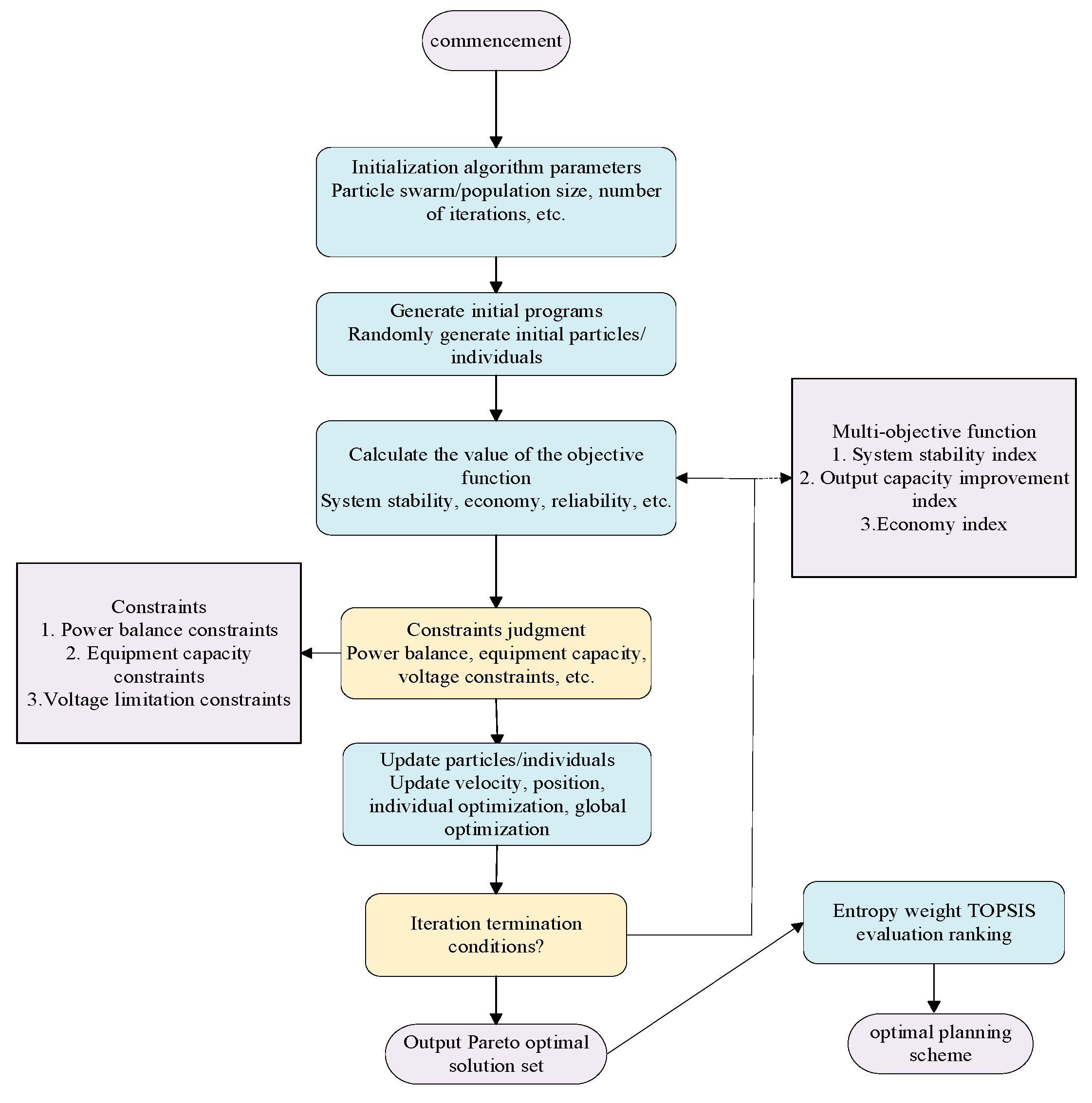
The multi-objective particle swarm optimization (MOPSO) algorithm was employed to resolve conflicting objectives and generate Pareto-optimal solutions. Key steps include:

Initialization: Generate candidate solutions (x) via randomized sampling within feasible domains.

Fitness evaluation: Compute objective function values (Equations (16)–(18)) and validate constraints.

Pareto front update: Maintain non-dominated solutions using crowding distance metrics to ensure diversity.

Velocity/position update: Adjust candidate solutions iteratively using particle swarm dynamics.

Termination: Output Pareto-optimal solutions upon reaching convergence criteria or iteration limits.

The optimization workflow is depicted in Figure 5, illustrating sequential stages from candidate generation, objective evaluation, and Pareto front refinement to final solution selection. The flowchart explicitly aligns algorithmic steps with mathematical formulations, demonstrating the systematic integration of MOPSO into the planning framework.

4. Coordinated Operation Strategy Design

4.1. System-Level Coordinated Operation Model

The system-level coordinated operation model explicitly accounts for interactions among various control devices and uncertainties introduced by renewable energy integration. The model is grounded in the fundamental principles of active and reactive power balance across the grid. A risk indicator is incorporated to quantify potential security threats under fault or renewable energy fluctuation scenarios. The overall objective function combines economic costs and security risks through weighted summation, expressed as:

$$\underset{u}{\min }F(u)=\alpha \cdot F_{econ}(u)+\beta \cdot F_{risk}(u)$$

(35)

where the decision variables u include the operating states and output parameters of control devices such as the novel FACTS units, traditional UPFCs, and VSC-HVDC systems. Fecon(u) represents the economic operation costs (e.g., generation, dispatch, and operational losses), while Frisk(u) quantifies the risks arising from line overloads, voltage deviations, and other security concerns. Weighting coefficients α and β balance economic efficiency against security, ensuring that the final dispatch strategy minimizes costs while maintaining system stability.

Wind uncertainty was modeled via Weibull distribution (k = 2, λ = 12 m/s) as per the China Meteorological Administration 2024 Jiangsu coastal wind data. The probabilistic risk metric is:

$$R(u)=\sum _{k=1}^K{p}_k\cdot r_k(u)$$

(36)

where p_k denotes the probability of disturbance scenario k, r_k(u) represents the risk metric (e.g., line overload or voltage deviation) under scenario k, and k is the total number of considered disturbance scenarios. This probabilistic framework captures the operational uncertainties under multiple disturbance conditions, providing safety constraints for subsequent coordinated dispatch.

The model must also satisfy nodal power balance constraints. For each node i, active and reactive power balance equations are defined as:

$$P_i^{gen}(u)-P_i^{load}=\sum _{i\subset N}{V}_i{V}_j\left(G_{ij}\cos {\theta }_{ij}+B_{ij}\sin {\theta }_{ij}\right),i\in N$$

(37)

$$Q_i^{gen}(u)-Q_i^{load}=\sum _{j\in N}{V}_i{V}_j\left(G_{ij}\sin {\theta }_{ij}-B_{ij}\cos {\theta }_{ij}\right),i\in N$$

(38)

where $P_i^{gen}(u)$ and $Q_i^{gen}(u)$ denote the active and reactive power injections from the generators and control devices at node i, $P_1^{\mathrm{load}}$ and $Q_i^{\mathrm{load}}$ represent the load demands, Vi is the voltage magnitude, θij = θi − θj is the phase angle difference, and Gij and Bij are the line conductance and susceptance, respectively. Equations (4) and (5) form the foundation of the coordinated operation model, ensuring global power balance under diverse disturbance conditions.

To reflect the topology-switching capability of the novel FACTS device, a converter status variable sk was introduced. The converter’s power injection is adjusted based on its operational state:

$$P_k^{\mathrm{inj}}(u)=s_k\cdot P_k^{\mathrm{nom}}(u),$$

(39)

This formulation dynamically models the power injection changes due to converter failures or shutdowns, ensuring post-fault power balance. By integrating the converter status variables with operational parameters, the model effectively captures the control characteristics of the novel FACTS device across multiple operating modes.

4.2. Coordinated Dispatch Algorithm Design

To solve the nonlinear, multi-objective, and constraint-rich dispatch problem, a coordinated dispatch strategy combining multi-objective particle swarm optimization (MOPSO) with a probabilistic model was proposed. The algorithm begins by randomly generating initial candidate solutions within the decision variable space. Each candidate solution x includes parameters such as the location, installed capacity, converter output settings, and switching states of the novel FACTS devices. Latin hypercube sampling (LHS) was employed to ensure the uniform distribution of solutions while adhering to the nodal power balance constraints:

$$P_i^{gen}(x)-P_i^{load}=\sum _{j\in N}{V}_i{V}_j\left(G_{ij}\cos {\theta }_{ij}+B_{ij}\sin {\theta }_{ij}\right),i\in N$$

(40)

$$Q_i^{gen}(x)-Q_i^{load}=\sum _{j\in N}{V}_i{V}_j\left(G_{ij}\sin {\theta }_{ij}-B_{ij}\cos {\theta }_{ij}\right),i\in N$$

(41)

Each candidate solution undergoes fitness evaluation, which incorporates economic costs and security risks:

$$F(x)=\alpha F_{econ}(x)+\beta F_{risk}(x),$$

(42)

where Fecon(x) includes the generation costs, dispatch costs, and operational losses, while Frisk(x) quantifies the risks using the probabilistic model in Equation (3).

$$F_{risk}(x)=\sum _{k=1}^K{p}_k{r}_k(x),$$

(43)

Here, pk denotes the occurrence probability of disturbance scenario k, and rk(x) represents the risk metric under this scenario such as line overloads or node voltage deviations. To enhance the granularity of fitness evaluation, the algorithm introduces an additional constraint penalty term. When a candidate solution x violates fundamental constraints, its fitness is adjusted via the penalty function Ppen(x), with the correction formula expressed as:

$$\tilde{F}(x)=F(x)+\lambda \cdot P_{pen}(x),$$

(44)

Here, the penalty function Ppen(x) quantifies the degree of constraint violations such as converter current exceeding limits or node voltage exceeding safe thresholds. The penalty coefficient λ is adaptively adjusted to ensure that violating solutions receive sufficiently high penalties.

After fitness evaluation, all candidate solutions undergo Pareto sorting based on multi-objective optimization principles. In addition to economic cost and risk objectives, a crowding distance di is introduced to maintain solution diversity. The crowding distance is calculated as:

$$d_i=\sum _{j=1}^n{\displaystyle \frac{|f_j(x_{i+1})-f_j(x_{i-1})|}{f_j^{\max }-f_j^{\min }}},$$

(45)

Here, fj(x) denotes the j-th objective function, and fjmax and fjmin represent the maximum and minimum values of the j-th objective function in the current solution set, respectively. The updated Pareto solution set provides reference information for subsequent particle swarm exploration.

During the particle swarm optimization (PSO) phase, each candidate solution is treated as a particle. The position vector xi(t) represents the solution parameters, and the velocity vector vi(t) defines the direction and step size within the solution space. The algorithm adjusts the velocity and position of particles using the following update equations:

$$v_i^{(t+1)}={\omega }^{(t)}{v}_i^{(t)}+c_1{r}_1\left(p_i^{\mathrm{best}}-x_i^{(t)}\right)+c_2{r}_2\left(g^{\mathrm{best}}-x_i^{(t)}\right),$$

(46)

$$x_i^{(t+1)}=x_i^{(t)}+v_i^{(t+1)},$$

(47)

Here, $p_i^{best}$ represents the historically optimal position of particle i, gbest denotes the optimal solution selected from the global non-dominated solution set, c1 and c2 are the cognitive and social learning factors, r1 and r2 are uniformly distributed random numbers introducing stochasticity, and ω(t) is the adaptive inertia weight. The adaptive inertia weight is updated using the following formula:

$${\omega }^{(t)}={\omega }_{\max }-\left({\omega }_{\max }-{\omega }_{\min }\right){\displaystyle \frac{t}{t_{\max }}},$$

(48)

Here, ωmax and ωmin represent the initial and minimum values of the inertia weight, t denotes the current iteration count, and tmax is the maximum number of iterations. This formula ensures that particles exhibit strong exploration capability in the early stages and gradually converge to local search in later stages, thereby improving the overall search efficiency.

To further enhance the algorithm’s local search capability and population diversity, a local neighborhood learning mechanism was introduced. Each particle not only references its own historical best position ($p_i^{best}$) and the global best solution (gbest), but also considers the optimal solutions within its neighborhood. Let $l_i^{best}$ denote the local neighborhood optimal solution. The particle update formula is then modified as:

$$v_i^{(t+1)}={\omega }^{(t)}{v}_i^{(t)}+c_1{r}_1\left(p_i^{\mathrm{best}}-x_i^{(t)}\right)+c_2{r}_2\left(g^{\mathrm{best}}-x_i^{(t)}\right)+c_3{r}_3\left(l_i^{\mathrm{best}}-x_i^{(t)}\right),$$

(49)

Here, c3 is the local learning factor, and r3 is a random factor. The introduction of Equation (42) enables the particle swarm to better capture high-quality solutions within local regions, avoid premature convergence to the local optima, and accelerate fine-grained solution refinement.

After each update, all newly generated candidate solutions undergo constraint checks. If a candidate solution violates constraints, such as system power balance, converter current limits, or node voltage thresholds, it is either projected back into the feasible region or corrected via the penalty function. The penalty function is typically formulated as:

$$P_{pen}(x)=\sum _j{\eta }_j\max {\{0,g_j(x)\}}^2,$$

(50)

where gj(x) ≤ 0 denotes the j-th constraint condition, and ηj is the corresponding penalty coefficient. By incorporating the penalty function, the algorithm effectively distinguishes feasible solutions from infeasible ones, ensuring that constraint-violating solutions receive higher penalties during fitness evaluation and are subsequently eliminated.

The particle swarm optimization process iteratively updates the fitness values, Pareto front, and crowding distance information of candidate solutions until the convergence criteria are met. Convergence can be determined based on the rate of change in global fitness or the stabilization of the non-dominated solution count over consecutive generations. Upon convergence, the algorithm terminates and outputs the final Pareto optimal solution set, offering decision-makers the optimal trade-offs between economic efficiency and security.

5. Simulation Analysis

To validate the effectiveness of the proposed novel FACTS device and its coordinated dispatch strategy, simulation studies were conducted on both the IEEE 39-bus system and a practical 500 kV power grid. The experiments encompassed steady-state power flow optimization, power loss analysis, node voltage stability, dynamic response characteristics, and economic operation optimization. Detailed explanations of the simulation results are provided below, accompanied by graphical descriptions and relevant computational formulas.

The simulation framework employed rigorously validated parameters to ensure credibility and reproducibility. Converter ratings were specified at ±50 MVA. Switching delays ranging from 2 to 5 milliseconds were implemented based on the manufacturer’s specifications documented in the ABB TN-203 technical manuals. Wind power fluctuation characteristics adopted a Beta(2,2) distribution, faithfully replicating the statistical patterns observed in Jiangsu grid’s 2022 operational data as presented in Reference [3]. Load profiles followed the CIGRE industrial benchmark curves published in Technical Brochure 876, ensuring realistic representation of the demand variations. These carefully selected parameters, grounded in industry standards and regional operational data, provide a robust foundation for the subsequent simulation scenarios examining the performance of the proposed FACTS device under realistic grid conditions.

In the steady-state simulations, three operating conditions were defined: the base case (without FACTS devices), the conventional FACTS case (employing traditional devices such as SVC and TCSC), and the novel FACTS case (utilizing the proposed device).

For steady-state power flow optimization, the series-connected converters operated at a ±50 MVA rating with 5 ms switching delay as documented in the technical manuals. The transmission line impedance scale was the 1.25× actual Jiangsu grid 2023 measurements.

Figure 6 illustrates the power flow data of key transmission lines (e.g., Line L12, L23, and L34) in the IEEE 39-bus system using a bar chart. The results show that under the base case, the power flow of certain lines approached their thermal limits. While the conventional FACTS case improved the power flow distribution to some extent, localized overloads persisted. In contrast, the novel FACTS case significantly reduced the power flow burden on heavily loaded lines, achieving a more balanced system-wide power flow distribution.

The proposed novel FACTS scheme reduced the ΔP by 22.8%, demonstrating its superiority in optimizing the power flow distribution.

Figure 7 presents line charts showing the time-domain curves of the total active power loss under three operating conditions as the load varied. The results indicate that the system loss was highest under the base case (without FACTS devices). While the conventional FACTS case moderately reduced the loss, the novel FACTS case achieved an approximately 8.5% reduction in total active power loss. The power loss was calculated using the formula:

In the dynamic response analysis, the study focused on the system’s behavior under two types of disturbances: wind power fluctuations and load step changes.

Dynamic response analysis incorporated 15% wind power penetration with Beta(2,2) distribution fluctuations. Load step changes implemented ±8% variations using standardized CIGRE Curve 7b profiles.

Figure 8 displays line charts comparing the system frequency deviation (unit: Hz) over time under wind power fluctuation scenarios for the three operating conditions. The x-axis represents time, while the y-axis indicates frequency deviation. The results show that the system frequency fluctuated severely in the base case (without FACTS devices). Although the conventional FACTS case mitigated these fluctuations, the novel FACTS case effectively suppressed frequency deviations, reducing the frequency oscillations by 43.2%. The theoretical model of system frequency response is also illustrated:

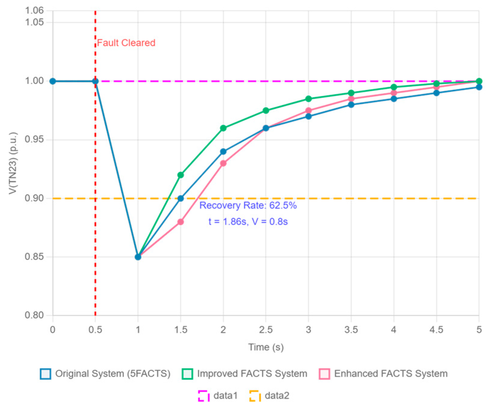
Figure 9 presents line charts illustrating the voltage recovery process at critical nodes over time under load step change scenarios. The results show that the novel FACTS device significantly accelerated the voltage recovery process, reducing the recovery time constant τ by approximately 40% compared with the conventional solution. The voltage recovery dynamics were modeled using an exponential decay function:

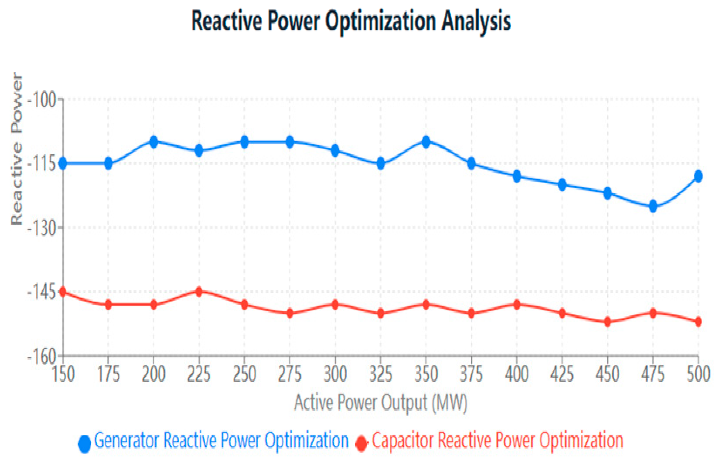
Figure 10 illustrates the variation in the reactive power output from FACTS devices over time under dynamic disturbances. Multiple curves were plotted to compare the performance of conventional and novel FACTS devices. The results demonstrate that the novel FACTS device rapidly adjusted its reactive power output within a short timeframe, effectively maintaining voltage stability at critical nodes. Its reactive power response exhibited smoother amplitude variations and shorter response times, providing robust support for system voltage regulation.

In terms of economic operation and optimal configuration, the study employed a multi-objective optimization algorithm to optimize the placement and operational parameters of FACTS devices.

Economic optimization applied α = 0.6 (security) and β = 0.4 (economy) weighting coefficients as per the State Grid operational standards. The 15-year device lifetime assumption aligned with the IEC 62305 recommendations.

Figure 11 presents line charts comparing the system operating costs (unit: 10⁴ CNY) under different optimization methods: conventional dispatch, genetic algorithm (GA), and MOPSO. The x-axis denotes the optimization schemes, while the y-axis represents the operating cost. The results demonstrate that the novel FACTS scheme, optimized using the proposed strategy, reduced the operating costs by approximately 12%. Additionally, the economic operation cost was calculated as:

Figure 12 uses scatter plots to display the Pareto front solution set obtained from multi-objective optimization. The x-axis represents the economic cost metric, and the y-axis denotes the security metric (e.g., voltage deviation or system risk), with each point corresponding to a Pareto-optimal solution. The results demonstrate that the novel FACTS scheme achieved a superior trade-off between economic efficiency and security compared with conventional solutions. The optimization objective function is provided in the figure:

Figure 13 illustrates the power flow variations of the key transmission lines during fault occurrence and recovery using line charts. The results showed that a sudden power flow change occurred at the instant of fault inception. With the intervention of the novel FACTS devices, the power flow rapidly recovered to normal levels. Comparative data demonstrated that the proposed scheme achieved shorter response times and appropriate regulation amplitudes, effectively mitigating the overload risks.

Building on the economic optimization results, this section provides a quantitative comparison with traditional UPFC and IPFC devices to comprehensively evaluate the performance of the proposed novel FACTS device.

Table 2. Comparative performance analysis.

Performance Metric	Traditional UPFC	Traditional IPFC	Proposed Novel FACTS
Cost analysis
Hardware cost ($/MVA)	45,000–55,000	50,000–60,000	48,000–52,000
Installation cost ($/MVA)	8000–12,000	10,000–14,000	9000–11,000
Maintenance cost ($/MVA/year)	1200–1500	1300–1600	900–1100
Response time analysis
Normal operation response	50–100 ms	60–120 ms	30–80 ms
Fault detection time	20–50 ms	25–60 ms	5–15 ms
Topology switching time	N/A	N/A	8–12 ms
Reconfiguration capabilities
Topology flexibility	Fixed	Fixed	Adaptive (4 modes)
Fault tolerance	Limited	Moderate	High
N-1 contingency support	No	Partial	Yes
Control performance
Power flow regulation accuracy	±2%	±2.5%	±1.5%
Voltage regulation range	±10%	±12%	±15%
Harmonic distortion (THD)	<5%	<5%	<3%

summarizes the key metrics across cost, response time, reconfiguration capabilities, and control performance, highlighting the superior advantages of the proposed device.

These quantitative results demonstrate that the proposed device significantly outperformed traditional solutions in cost-effectiveness, response speed, and reconfiguration capabilities, providing a data-driven foundation for subsequent engineering applications.

Through a comparative analysis of the simulation results, the following conclusions can be drawn:

The novel FACTS devices significantly improved the power flow distribution under steady-state operation, balancing the load on critical lines and reducing the power flow dispersion by 22.8%.

Total active power loss decreased by approximately 8.5% under the novel scheme, highlighting its effectiveness in reducing transmission losses and improving efficiency.

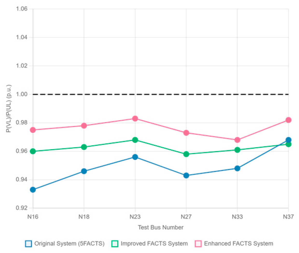
Voltage fluctuations at critical nodes were substantially reduced, with voltage deviation decreasing by 15%, validating the device’s capability in voltage stability regulation.

Under dynamic disturbances, the novel scheme suppressed the frequency deviations caused by wind power fluctuations by 43.2%. In load step change scenarios, the voltage recovery time was shortened by 40%, demonstrating superior dynamic response characteristics.

Optimization results revealed that the novel scheme reduced the economic operation costs by 12% through multi-objective optimization methods and achieved better trade-offs between economic efficiency and security on the Pareto front.

Overall, the novel FACTS devices and their coordinated dispatch strategy outperformed conventional solutions in steady-state/dynamic regulation, economic efficiency, and security, providing robust technical support and theoretical foundations for practical engineering applications.

The simulation analysis comprehensively compared and discussed five aspects: steady-state power flow, power loss, voltage stability, dynamic response, and economic operation. Over ten graphical results, numerical comparisons, formula derivations, and theoretical explanations collectively validated the advantages of the novel FACTS devices in enhancing system security, economic efficiency, and dynamic response capabilities. These findings establish a solid technical foundation and decision-making framework for future engineering implementations.

6. Conclusions

This paper proposed a novel FACTS device based on interline power flow control with coordinated planning and operational strategies. The hardware configuration (Figure 1 and Figure 2) featuring fault tolerance and topology switching capabilities overcomes control failure issues during N-1 contingencies. The steady-state modeling approach (Figure 3) accurately characterized electrical behaviors under multi-mode operation, while the entropy-weighted TOPSIS evaluation system (Figure 4) quantified comprehensive performance improvements after device integration. The coordinated optimization model (Figure 5) balanced economic and security objectives, and the system-level operational strategy effectively mitigated renewable uncertainties and fault risks. Jiangsu grid simulations demonstrated: (1) a 22.8% increase in key transmission corridor capacity; (2) 15% reduction in power flow imbalance; and (3) 40% shorter post-fault voltage recovery time.

Future work will extend the device to hybrid AC/DC grids and develop adaptive control strategies using deep reinforcement learning.