Dynamic Modeling and Online Updating of Full-Power Converter Wind Turbines Based on Physics-Informed Neural Networks and Bayesian Neural Networks

Abstract

This paper presents a dynamic model for full-power converter permanent magnet synchronous wind turbines based on Physics-Informed Neural Networks (PINNs). The model integrates the physical dynamics of the wind turbine directly into the loss function, enabling high-accuracy equivalent modeling with limited data and overcoming the typical “black-box” constraints and large data requirements of traditional data-driven approaches. To enhance the model’s real-time adaptability, we introduce an online update mechanism leveraging Bayesian Neural Networks (BNNs) combined with a clustering-guided strategy. This mechanism estimates uncertainty in the neural network weights in real-time, accurately identifies error sources, and performs local fine-tuning on clustered data. This improves the model’s ability to track real-time errors and addresses the challenge of parameter-specific adjustments. Finally, the data-driven model is integrated into the CloudPSS platform, and its multi-scenario modeling accuracy is validated across various typical cases, demonstrating the robustness of the proposed approach.

1. Introduction

As a pivotal platform for addressing global energy challenges, power systems are experiencing significant changes in their dynamic characteristics, driven by energy structure transformation and the large-scale integration of new energy technologies [1,2,3]. New energy devices, characterized by high levels of power electronics, can induce grid instabilities in extremely short timeframes, posing risks to the grid’s secure and stable operation. This underscores the importance of accurate new energy device modeling, which plays a critical role in ensuring grid safety, enhancing operational efficiency, and improving system reliability. Moreover, precise modeling of new energy systems is vital for supporting grid integration technologies, system planning, and market policy development. In modern power systems, particularly in the context of large-scale wind farm integration, the precision of new energy device modeling directly influences stability analysis and control performance. It is also a key enabler for the advancement of digital twin technologies [4].

Nevertheless, the large-scale integration of wind power has introduced greater complexity into the power system’s dynamic behavior [5,6], which now exhibits highly nonlinear and coupled characteristics. This adds new challenges to stability analysis. Specifically, power system modeling faces two primary difficulties: First, the lack of detailed prior knowledge and physical models. Due to factors such as proprietary technology, measurement limitations, and the complexity of system components, the internal structure and operating principles of many devices remain opaque, resulting in so-called “black-box” or “gray-box” models. Under these circumstances, traditional simulation methods struggle to accurately predict dynamic behavior [7]. Second, the dynamic characteristics of wind turbine systems are highly complex and of a high order, making it difficult to capture all relevant behaviors with simple low-order models. This complexity increases the challenges of model construction and restricts the application of these models in fast simulations and real-time control [8].

To overcome these challenges, data-driven modeling methods, combined with big data technologies and real-time measurement results, can effectively capture the dynamic characteristics of power systems. This approach not only enhances simulation accuracy but also provides robust support for system control and optimization. In the context of large-scale wind power integration, the application of data-driven models and simulation technologies will greatly improve the efficiency and stability of power system operations, promoting the development of smart grids. The integration of artificial intelligence (AI) techniques, particularly deep learning, into electromagnetic transient simulations has led to significant advancements in the data-driven modeling of wind farm equipment. Achieving accurate dynamic equivalence of device components remains a difficult task, and scholars have developed various methods to enhance performance in this area. Some studies, focused on port equivalence, have employed wide-area damping control (WADC) [9] and created surrogate models using neural networks for generators [10,11] and solar power plants [12]. However, neural network models built from limited data often neglect the internal structure of components. While these models demonstrate strong tracking capabilities under the conditions of the training dataset, they tend to perform poorly under unknown conditions [13].

In recent years, researchers have begun combining the physical and dynamic characteristics of power systems with deep learning technologies [14,15], leading to the development of more interpretable and effective deep learning models. Physics-Informed Neural Networks (PINNs) have already been applied in power systems. For example, ref. [16] introduced a deep Koopman method, where neural networks learn the Koopman operator that encapsulates system properties, enabling dynamic predictions of components within a high-dimensional linearized space. When partial boundary conditions and system dynamics are known, a Physics-Informed Neural Network (PINN) was introduced [17]. Refs. [18,19] applied PINNs to electromagnetic problems, with experiments showing that PINNs, by integrating high-frequency and topological information, excel in solving high-dimensional, parameterized problems. Refs. [20,21] validated the performance of PINNs in simulations of heat conduction, wave equations, and thermal inversion, demonstrating their efficiency in handling two-dimensional transient problems with low computational costs and ease of implementation. Ref. [22] also proposed a method for transient stability analysis of power systems using PINNs, which showed high efficiency and accuracy when applied to electromechanical transient simulations over longer time scales. Although previous studies have demonstrated that microsecond-level electromagnetic dynamics can be modeled using PINNs within a single domain, power systems are inherently large-scale and feature complex multi-domain coupling dynamics. Additionally, existing simulation platforms are rigid in interface design and lack compatibility with diverse model types, leading to the absence of a mature framework that integrates data-driven and physics-driven modeling approaches. To address these challenges, this paper proposes a PINN-based method for dynamic modeling and integrated co-simulation of wind farms.

The key contributions of this paper are as follows:

• A dynamic model for full-power converter permanent magnet synchronous generators (PMSGs) is developed based on Physics-Informed Neural Networks (PINNs). This model explicitly incorporates the physical dynamics of the wind turbine into the error function, allowing high-precision equivalent modeling with small-scale data. This approach addresses the “black-box” limitations and high data requirements typically associated with data-driven modeling.
• An online updating mechanism for data-driven models is introduced, leveraging Bayesian neural networks (BNNs) and a clustering-guided strategy. This mechanism accurately identifies sources of bias by estimating the uncertainty in the weights of each neural network layer in real-time. Based on this, targeted local fine-tuning is performed on clustered data, improving the model’s ability to track errors in real-time and solve targeted parameter fine-tuning challenges.
• A data-driven model integration interface is implemented on the CloudPSS platform, where its multi-scenario modeling accuracy is verified through various typical scenarios, confirming the robustness of the proposed model.

2. Harmonic State-Space-Based Modeling for Direct-Drive Wind Power Systems

The Harmonic State Space (HSS) method [23,24] offers a substantial reduction in the computational complexity of Linear Time Periodic (LTP) systems by converting their time-domain state equations into linear time-invariant (LTI) state equations in the frequency domain. Compared to the dynamic phasor approach, HSS modeling is more streamlined, avoiding intricate formula derivations. Moreover, HSS formulates dynamic harmonic phasors in the complex domain, unlike the dynamic phasor method, which treats real and imaginary parts separately. Consequently, after linearization, HSS can directly obtain the small-signal impedance model, which aids in analyzing the system’s resonance characteristics and stability.

The state-space model for a Linear Time Periodic (LTP) system is typically represented as

$$\begin{array}{cc}\hfill & \dot{x}\left(t\right)=A\left(t\right)x\left(t\right)+B\left(t\right)u\left(t\right)\hfill \\ \hfill & y\left(t\right)=C\left(t\right)x\left(t\right)+D\left(t\right)u\left(t\right)\hfill \end{array}$$

(1)

where $x\left(t\right)$ and $u\left(t\right)$ denote the state and input variables, respectively. $A\left(t\right)$, $B\left(t\right)$, $C\left(t\right)$, and $D\left(t\right)$ are periodic with a period $T_0$. The time periodic signal $x\left(t\right)$ can be expanded as a Fourier series:

$$x\left(t\right)=\sum _{h=-\infty }^{\infty }{X}_h\left(t\right)e^{jh{\omega }_{0}t}$$

(2)

where h denotes the harmonic order, and ${\omega }_0=2\pi f$, with $f=50\mathrm{Hz}$. The Fourier coefficient $X_k\left(t\right)$ is given by

$$X_k\left(t\right)={\displaystyle \frac{1}{T}}{\int }_{t_0}^{t_0+T}x\left(t\right)e^{-jk{\omega }_{0}t}dt$$

(3)

Taking into account the differential properties of periodic signals, the HSS model is derived as

$$\left\{\begin{array}{c}\dot{X}=(\Gamma \left(A\right)-N)X+\Gamma \left(B\right)U\hfill \\ Y=\Gamma \left(C\right)X+\Gamma \left(D\right)U\hfill \end{array}\right.$$

(4)

where $\Gamma (·)$ are the Toeplitz matrices, and $\Gamma \left(A\right)$, $\Gamma \left(B\right)$, $\Gamma \left(C\right)$, and $\Gamma \left(D\right)$ are the Toeplitz matrices of A, B, C, and D, while N is defined as

$$N=\mathrm{diag}\left[-jh\omega ,\dots ,-j\omega ,0,j\omega ,\dots ,jh\omega \right]$$

(5)

where diag $(·)$ is a diagonal matrix. From the above modeling procedure, it is evident that HSS provides a straightforward and efficient approach, avoiding complex derivations. By transforming an LTP system into an LTI system, the harmonic phasors in (4) enable an intuitive and precise analysis of harmonic generation and propagation during transients.

In a permanent magnet synchronous generator (PMSG) system, the grid-side converter (GSC) operates using constant DC voltage control, while the machine-side converter (MSC) is governed by speed control. The control topology for the grid-side converter is illustrated in Figure 1.

The HSS model for the voltage outer loop is

$$\left\{\begin{array}{c}{i}_{dref\_gsc}=k_{gsc\_p}(u_{dcref\_gsc}-u_{dc\_gsc})+k_{gsci}{x}_{gsc\_dc}\hfill \\ {\displaystyle \frac{d{x}_{gsc\_dc}}{dt}}=-N{x}_{gsc\_dc}+(u_{dcref\_gsc}-u_{dc\_gsc})\hfill \end{array}\right.$$

(6)

where $u_{dc\_gsc}$ represents the DC capacitor voltage, $u_{dcref\_gsc}$ represents the reference value of the DC-side voltage, $i_{dref\_gsc}$ and $i_{qref\_gsc}$ represent the current reference values for the inner current loop, and $k_{gscp\_gsc}$ and $k_{gsci\_gsc}$ represent the PI control parameters for the outer loop.

The HSS model for the current loop is

$$\begin{array}{cc}\hfill U_{gsc\_d}& =\Gamma \left(\omega \right)L_{gsc}{i}_{q_{gsc}}+k_{gscip}\left(i_{dre{f}_{gsc}}-i_{d_{gsc}}\right)+k_{gscii}{x}_{gscd}\hfill \end{array}$$

(7)

$$\begin{array}{cc}\hfill U_{gsc\_q}& =\Gamma \left(\omega \right)L_{gsc}{i}_{d_{gsc}}+k_{gscip}\left(0\ast EI-i_{q_{gsc}}\right)+k_{gscii}{x}_{gscq}\hfill \end{array}$$

(8)

$$\begin{array}{cc}\hfill {\displaystyle \frac{d{x}_{gsc\_d}}{dt}}& =-N{x}_{gsc\_d}+\left(i_{dref\_gsc}-i_{d_{gsc}}\right)\hfill \end{array}$$

(9)

$$\begin{array}{cc}\hfill {\displaystyle \frac{d{x}_{gsc\_q}}{dt}}& =-N{x}_{gsc\_q}+\left(i_{qref\_gsc}-i_{q_{gsc}}\right)\hfill \end{array}$$

(10)

where $U_{gsc\_d}$ and $U_{gsc\_q}$ denote the output modulation voltages corresponding to the d-axis and q-axis, respectively. The HSS model for the PLL is

$$\begin{array}{cc}\hfill \omega & ={\omega }_0+k_{pll}^p{u}_q+k_{pll}^i{x}_{pll}\hfill \end{array}$$

(11)

$$\begin{array}{cc}\hfill {\displaystyle \frac{d{x}_{pll}}{dt}}& =-N{x}_{pll}+u_q\hfill \end{array}$$

(12)

$$\begin{array}{cc}\hfill {\displaystyle \frac{d{\theta }_{PLL}}{dt}}& =-N\Delta {\theta }_{PLL}+\omega \hfill \end{array}$$

(13)

3. Intelligent Modeling of PMSG Based on PINNs

This paper employs PINNs to model PMSG systems. PINNs integrate physical equations, such as the electromagnetic and mechanical dynamic equations of PMSGs, into the neural network’s loss function. This integration ensures that the network outputs remain consistent with physical laws, enhancing both model accuracy and physical interpretability. Compared to conventional deep learning models, PINNs reduce the dependency on large datasets by leveraging physical equations, allowing for high-precision modeling even in cases of limited data. Additionally, PINNs exhibit superior generalization capabilities under various operating conditions and unknown external environments, as they rely not only on data but also on the inherent physical properties of the system.

To construct a PINN that integrates the three sets of equations, it is necessary to combine the system’s dynamic equations with the neural network’s architecture and loss function. The PINN leverages neural networks to approximate unknown functions that represent the system’s state variables. In the context of the PMSG structure, the PINN takes as input variables t, $u_{dcref\_gsc}\left(t\right)$, $u_{dc\_gsc}\left(t\right)$, $i_{d_{gsc}}\left(t\right)$, $i_{q_{gsc}}\left(t\right)$, and $u_q\left(t\right)$. The output variables are $i_{dref\_gsc}\left(t\right)$, $x_{gscdc}\left(t\right)$, $x_{gscd}\left(t\right)$, $x_{gscq}\left(t\right)$, $U_{gs{c}_d}\left(t\right)$, $U_{gs{c}_q}\left(t\right)$, $x_{pll}\left(t\right)$, $\omega \left(t\right)$, and ${\theta }_{PLL}\left(t\right)$.

The core principle of PINN is embedding the residuals of the physical equations into the loss function. These residuals quantify the degree to which the neural network’s predicted outputs align with the differential equations. Thus, nine residuals incorporating the physical dynamics are constructed as follows:

• Voltage outer loop residuals

  $$R_1\left(t\right)=i_{dref\_gsc}^{NN}\left(t\right)-k_{gscp}(u_{dcref\_gsc}\left(t\right)-u_{dc\_gsc}\left(t\right))-k_{gsci}{x}_{gscdc}^{NN}\left(t\right)$$

  (14)

  $$R_2\left(t\right)={\displaystyle \frac{d}{dt}}{x}_{gscdc}^{NN}\left(t\right)+N{x}_{gscdc}^{NN}\left(t\right)-(u_{dcref\_gsc}\left(t\right)-u_{dc\_gsc}\left(t\right))$$

  (15)

  where the superscript $NN$ indicates the variables predicted by the neural network.
• Current inner loop residuals

  $$R_3\left(t\right)=U_{gs{c}_d}^{NN}\left(t\right)-[\Gamma \left({\omega }^{NN}\left(t\right)\right)L_{gsc}{i}_{q_{gsc}}\left(t\right)+k_{gscip}(i_{dref\_gsc}^{NN}\left(t\right)-i_{d_{gsc}}\left(t\right))+k_{gscii}{x}_{gscd}^{NN}\left(t\right)]$$

  (16)

  $$R_4\left(t\right)=U_{gs{c}_q}^{NN}\left(t\right)-[\Gamma \left({\omega }^{NN}\left(t\right)\right)L_{gsc}{i}_{d_{gsc}}\left(t\right)+k_{gscip}(i_{qre{f}_{gsc}}\left(t\right)-i_{q_{gsc}}\left(t\right))+k_{gscii}{x}_{gscq}^{NN}\left(t\right)]$$

  (17)

  $$R_5\left(t\right)={\displaystyle \frac{d}{dt}}{x}_{gscd}^{NN}\left(t\right)+N{x}_{gscd}^{NN}\left(t\right)-(i_{dref\_gsc}^{NN}\left(t\right)-i_{d_{gsc}}\left(t\right))$$

  (18)

  $$R_6\left(t\right)={\displaystyle \frac{d}{dt}}{x}_{gscq}^{NN}\left(t\right)+N{x}_{gscq}^{NN}\left(t\right)-(i_{qref\_gsc}\left(t\right)-i_{q_{gsc}}\left(t\right))$$

  (19)
• PLL residuals

  $$R_7\left(t\right)={\omega }^{NN}\left(t\right)-[{\omega }_0+k_{pll}^p{u}_q\left(t\right)+k_{pll}^i{x}_{pll}^{NN}\left(t\right)]$$

  (20)

  $$R_8\left(t\right)={\displaystyle \frac{d}{dt}}{x}_{pll}^{NN}\left(t\right)+N{x}_{pll}^{NN}\left(t\right)-u_q\left(t\right)$$

  (21)

  $$R_9\left(t\right)={\displaystyle \frac{d}{dt}}{\theta }_{PLL}^{NN}\left(t\right)+N\Delta {\theta }_{PLL}\left(t\right)-{\omega }^{NN}\left(t\right)$$

  (22)

Finally, the loss function $\mathcal{L}$ is

$$\mathcal{L}=\sum _{i=1}^9{∥R_i\left(t\right)∥}^2$$

(23)

4. A Local Data Fine-Tuning Strategy Based on Bayesian Neural Networks

To improve the model’s real-time adaptability, a local data fine-tuning strategy based on Bayesian Neural Networks (BNNs) is introduced. This strategy involves measuring the cosine similarity between real-time power data and historical reference data to detect deviations in the data distribution, which then trigger localized model adjustments. BNNs are employed to estimate the uncertainty in the weights or outputs of each neural network layer, identifying the regions with the highest error deviations. These areas are then fine-tuned in subsequent steps to better accommodate new incoming data.

4.1. PMSG Sample Data Deviation Measurement Based on Cosine Similarity

The data in PMSG systems often exhibit high-dimensional and complex spatiotemporal properties. Cosine similarity is effective in capturing directional similarities between input vectors, making it especially suitable for analyzing features in high-dimensional spaces. When the cosine similarity between a new input sample $x_t$ and a historical reference sample $y_h$ falls below a predefined threshold ${\theta }_{\mathrm{threshold}}$, this indicates a significant deviation between the current system state and its historical state, triggering the model’s local fine-tuning mechanism. If the similarity is high, the model can use a smaller update step ${\eta }_{\mathrm{small}}$ for local fine-tuning, expressed as

$${\theta }_{new}={\theta }_{old}-{\eta }_{\mathrm{small}}{\nabla }_{\theta }\mathcal{L}(x_t,y_h)$$

(24)

where ${\nabla }_{\theta }\mathcal{L}(x_t,y_h)$ denotes the gradient of the loss function computed based on the current sample $x_t$ and the reference sample $y_h$. When the similarity is low, the model requires a larger update step ${\eta }_{\mathrm{large}}$ to perform stronger local adjustments:

$${\theta }_{new}={\theta }_{old}-{\eta }_{\mathrm{large}}{\nabla }_{\theta }\mathcal{L}(x_t,y_h)$$

(25)

4.2. Online Model Error Tracking Using Bayesian Neural Networks

Once the data for local fine-tuning are identified, the output is dynamically updated using Bayesian Neural Networks (BNNs). For a particular layer, the current input PMSG sample data are denoted by $x_l$, the observed output by $o_l$, and the weights by $w_l$. The output of this layer is expressed as

$$o_l=f\left(x_l;w_l\right)$$

(26)

where f represents the activation function of the layer. In Bayesian Neural Networks, the weight $w_l$ is modeled as a probability distribution instead of a fixed value, usually assumed to follow a normal distribution:

$$w_l\sim \mathcal{N}({\mu }_l,{\sigma }_l^2)$$

(27)

where ${\mu }_l$ is the mean of the weight, while ${\sigma }_l^2$ represents the standard deviation, indicating the uncertainty of the weight. During real-time dynamic data collection and tracking, the distribution of the weight $\omega$ must be adjusted according to the current data distribution. The Bayesian Neural Network calculates the new weight and the variance of the output as

$${\sigma }_w^2=\mathrm{Var}\left(w\right),{\sigma }_y^2=\mathrm{Var}\left(y\right)$$

(28)

By estimating the uncertainty in the weights and outputs of each layer, Bayesian Neural Networks (BNNs) can identify the parts of the network with the largest output error deviations for further fine-tuning, allowing the model to better adapt to new data. The uncertainty is typically quantified using the variance of the posterior distribution, ${\sigma }_l^2$. For each layer’s output, $o_l$, the output uncertainty ${\sigma }_{ol}^2$ is calculated as

$${\sigma }_{o_l}^2={\left({\displaystyle \frac{\partial o_l}{\partial w_l}}\right)}^2·{\sigma }_l^2$$

(29)

When the output uncertainty in a particular layer exceeds the predefined threshold ${\theta }_{\mathrm{uncertainty}}$, that layer is identified as the source of error. The weights or outputs in this part of the network will then become the focus for local optimization or fine-tuning in the next step.

5. Case Study

5.1. Simulation Experiment Setup

This paper develops a full electromagnetic transient simulation model of the permanent magnet synchronous generator (PMSG) on the CloudPSS cloud simulation platform to validate the effectiveness of the proposed method. The software environment used for verification includes Python 3.8 and TensorFlow 2.08, with training samples simulated on this platform. The CloudPSS platform, developed by Tsinghua University, is a cloud-based simulation platform for electromagnetic transients in power systems. It features high computational performance, strong code compatibility, and supports large-scale parallel simulations. Given that this paper involves the joint simulation of mechanistic and data-driven models, the platform was chosen for simulation validation. The simulation hardware configuration consists of an China Intel i9-13900K CPU, 32 GB of memory, and an China NVIDIA A40 48 GB GPU. The sample set used in the simulations includes steady-state conditions, asymmetrical faults at the PMSG connection point, and three-phase faults, totaling 500 samples. The simulation step size is set to 50 microseconds (50 μs).

5.2. Structure and Parameters of PINNs and BNNs

The specific network structures and hyperparameters for the PINNs and BNNs used in this paper are presented in

Table 1. Hyperparameter settings for PINNs.

Hyperparameter	Value	Hyperparameter	Value
Hidden layer type	2D-Conv layer	Training epochs	1000
Filters	[16, 4, 1]	Activation	[ReLU, ReLU, ReLU]
Kernel size	[3, 3, 3]	Learning rate	1E-4
Padding	’Same’	Batch size	128
Constraint strength $\beta$	0.01	Regularization proportion $\rho$	0.6

and

Table 2. Hyperparameter settings for BNNs.

Hyperparameter	Value	Hyperparameter	Value
Hidden layer type	FC layer	Training epochs	1000
Dimension of hidden layers	[24, 32, 32, 24]	Activation function	[ReLU, ReLU, ReLU]
Batch size	128	Learning rate ${\eta }_1$, ${\eta }_2$	[1E-4, 1E-6]
FL aggregation interval	5	predict step p	100

.

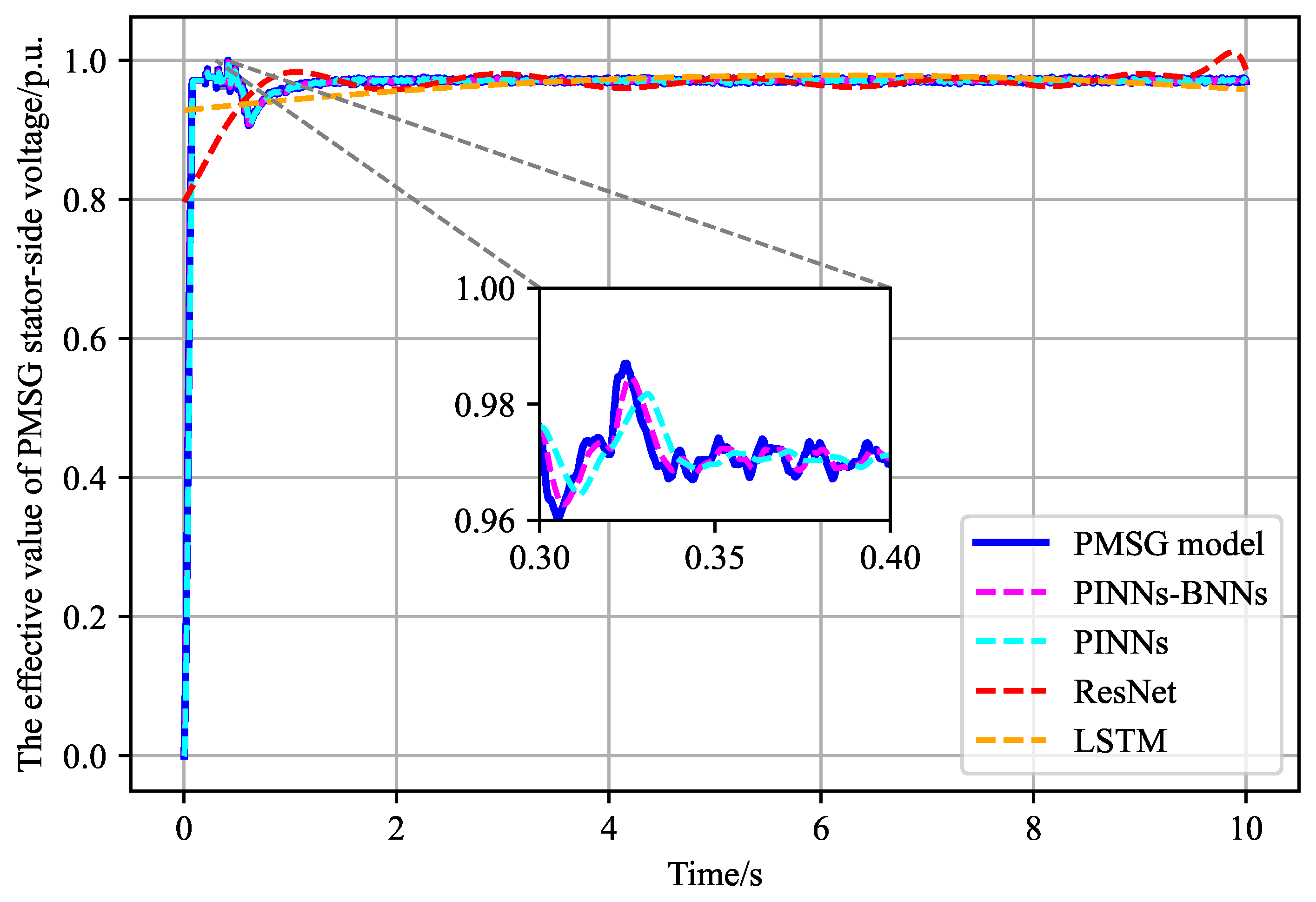
5.3. PMSG Steady-State Modeling Analysis

The electromagnetic transient simulation employs a zero-start strategy, starting from a zero state and running until the system stabilizes. To reach an operational steady state, the system must undergo a dynamic process of gradual power increase, which involves various nonlinear control and power regulation processes. Consequently, electromagnetic transient simulations are more nonlinear than electromechanical transient simulations. In this paper, PINNs, ResNet, and LSTM are used as comparison algorithms. The modeling results are presented in Figure 2 and

Table 3. Comparison of DC-side voltage errors in PMSG node stability.

Method	PINNs-BNNs	PINNs	ResNet	LSTM
MSE	5.598E-6	3.636E-5	2.124E-3	2.503E-3
MAE	6.710E-4	1.392E-3	1.372E-2	1.241E-2

and

Table 4. Training and testing cost comparison of data-driven wind farm modeling.

Model	Training Memory Usage (GB)	GPU Memory Usage (GB)	Training Time (Hours)	Testing Time (Seconds/Sample)
PINNs-BNNs	5–8	8–12	5–10	0.05
PINNs	3–5	3	4–7	0.03
ResNet	2.5	1	2–5	0.01
LSTM	3–4	2.5	3–6	0.02

.

MSE and MAE are commonly used metrics to assess model accuracy, providing different perspectives on how well the dynamics of an equivalent model developed using neural networks align with the dynamics of a precise model. As shown in Table 3, for MSE, the PINN-BNN model exhibits the smallest error, with a value of 5.598E-6, significantly outperforming the other models. The error for PINNs, used as the ablation control algorithm in the PINN-BNN experiment, is 3.636E-5, considerably larger than that of PINNs-BNNs. The errors for ResNet and LSTM are 2.124E-3 and 2.503E-3, respectively, with LSTM’s error being slightly higher than that of ResNet. For MAE, the trends mirror those of the MSE. The error for PINNs-BNNs is 6.710E-4, which is still the smallest. Figure 2 demonstrates that both PINNs-BNNs and PINNs are able to effectively track the nonlinear process during startup. In contrast, although ResNet and LSTM converge to similar steady-state operating points, their ability to accurately simulate the nonlinear process during startup is poor, indicating that they have not fully captured the dynamics of the PMSG. As shown in Table 4, the training cost of PINNs-BNNs is relatively the highest, primarily due to its larger network scale compared to single-network models. ResNet, with its characteristic residual structure, enables the construction of neural networks with fewer layers. Nevertheless, the PINNs network delivers superior performance while maintaining a training cost comparable to other models. Notably, PINNs and PINNs-BNNs are the only network types capable of effectively capturing the dynamics of wind farms. This underscores the effectiveness of the proposed approach. Furthermore, incorporating the BNNs is essential for further improving performance. Although this requires additional hardware resources, the increase is not substantial, allowing engineers to choose an appropriate network structure based on practical engineering needs.

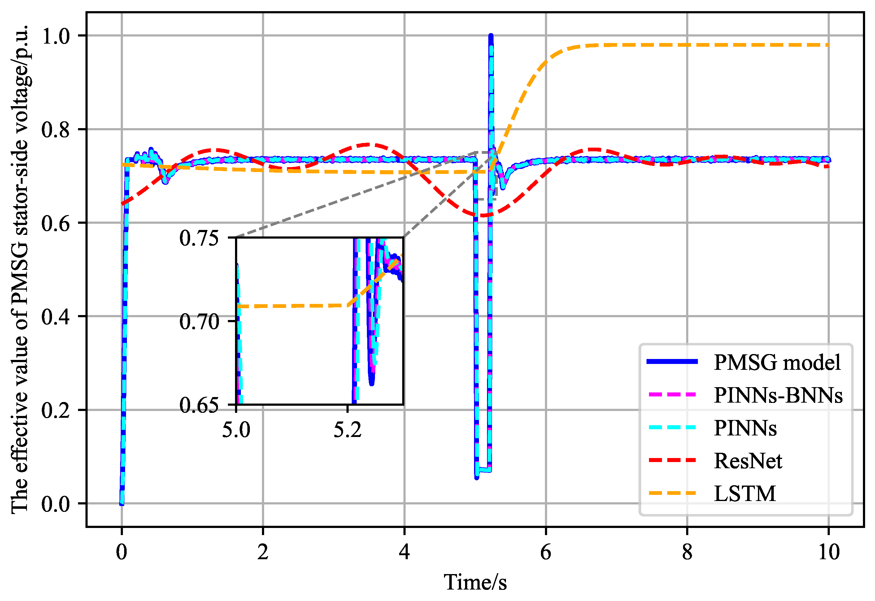
5.4. Analysis of PMSG Modeling Accuracy Under Unbalanced Large Disturbances

Electromagnetic transient analysis plays a crucial role in studying the microsecond-level dynamic behavior of high-renewable-energy penetration systems during disturbances. Unlike electromechanical transient simulations, it can account for rapid switching transitions and other influencing factors. This paper examines the modeling behavior of four different PMSG replacement models under such disturbances, specifically during a two-phase short-circuit fault at the PMSG grid connection point, as illustrated in Figure 3 and

Table 5. Comparison of errors under inter-phase short-circuit disturbance in PMSG grid-connected bus.

Method	PINNs-BNNs	PINNs	ResNet	LSTM
MSE	2.933E-5	1.867E-4	8.090E-3	3.464E-2
MAE	9.236E-4	2.116E-3	3.701E-2	1.334E-2

.

Under disturbance, the nonlinearity of the wind farm model significantly increases, placing higher demands on the feature capture capabilities of data-driven models. A short-circuit fault occurs at the PMSG grid connection point at 5 s, which is cleared 200 ms later. During the fault period, fault ride-through control will be activated. Among the four data-driven models, only the method proposed in this paper and PINNs can effectively simulate the low-voltage ride-through process, with the proposed method providing a more accurate simulation of voltage amplitude variations. ResNet struggles to model the dynamic characteristics of the wind turbine over the entire cycle, and LSTM fails to operate properly during faults, deviating significantly from the original stable operating point. Error analysis reveals a reduction in steady-state errors for the proposed method. However, it continues to exhibit the best error performance, outperforming the other three methods by approximately 1–2 orders of magnitude on average. Furthermore, compared to the ablation control group using PINNs, the MSE and MAE were improved by approximately 84.3% and 56.4%, respectively.

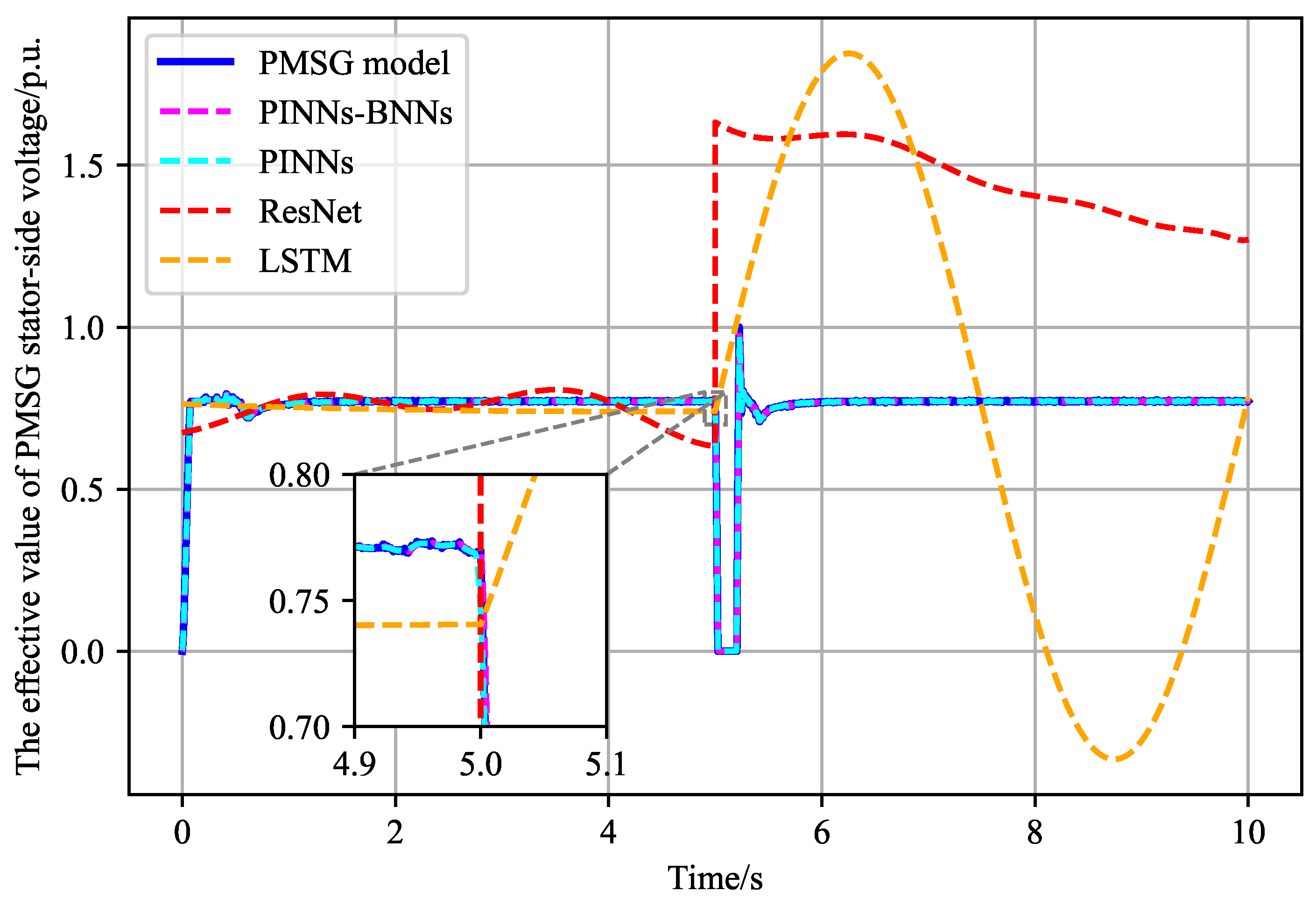
5.5. Modeling Accuracy Analysis of the PMSG Grid Connection Point Under Significant Three-Phase Disturbances

To further validate the model’s ability to accurately fit nonlinear characteristics under large disturbances, this paper simulates the response accuracy of several intelligent surrogate models during a three-phase short-circuit fault. The fault occurs at the PMSG grid connection point, with a fault duration of 200 ms. The modeling results from four different methods are presented in Figure 4 and

Table 6. Comparison of errors under three-phase short-circuit disturbances on the DFIG grid-connected bus.

Method	PINNs-BNNs	PINNs	ResNet	LSTM
MSE	3.419E-5	2.134E-4	2.828E-1	3.136E-1
MAE	9.654E-4	6.322E-3	3.788E-1	3.759E-1

.

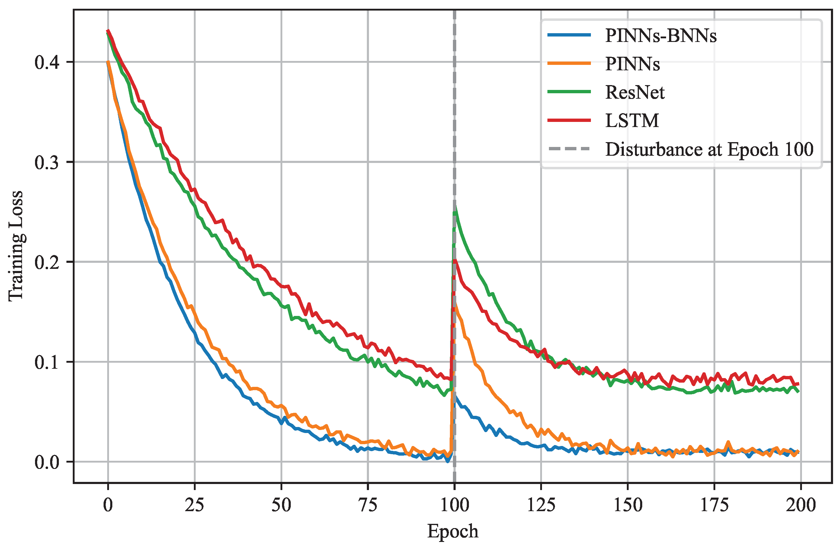
The active power curves modeled by the four methods shown in Figure 4 reveal that both the proposed method and the PINN-based model effectively maintain accuracy throughout the entire simulation time during the highly nonlinear three-phase short-circuit fault. In contrast, the models based on ResNet and LSTM networks suffer significant distortion after the occurrence of the three-phase fault. The ResNet-based model exhibits a step change of approximately 0.7 p.u., which decays over time, while the LSTM-based model experiences large-amplitude ultra-low-frequency oscillations following the disturbance, which clearly deviates from the dynamic characteristics of the accurate model. From an error analysis perspective, both the PINN and PINN-BNN models have errors below the 10E-3 magnitude. With the introduction of BNNs, PINNs-BNNs further reduce the MSE and MAE errors by approximately 83.98% and 84.73%, respectively. In contrast, the ResNet and LSTM models exhibit severe distortion, with MSE and MAE values at the 10E-1 level, indicating that the simulation has failed following a significant three-phase disturbance. Neural network training depends on precise parameter tuning guided by error signals. To evaluate the effectiveness of the proposed online model error tracking in identifying severely erroneous parameters during training, we designed an experiment. At the 100th epoch of each neural network’s training, we applied a targeted perturbation by inverting the weights ($\omega$ = $-\omega$) of an equal number of neurons. This manipulation caused a notable increase in prediction error. The networks then proceeded with training to correct this disturbance. The experimental results are presented in Figure 5.

The PINN and PINN-BNN approaches adopt an active update strategy that allows for the rapid detection of high-error regions in model parameters following perturbations, enabling swift corrective adjustments. Compared to other approaches, they achieve faster convergence and yield superior error performance upon convergence. These results indicate that the proposed strategy significantly improves both training efficiency and convergence behavior.

6. Conclusions

This paper presents a dynamic modeling approach for a full-power converter permanent magnet synchronous wind generator (PMSG), driven by an interpretable machine learning method. The approach offers strong interpretability and achieves notably higher accuracy in closed-loop simulations compared to existing methods. The key findings are as follows:

Physical constraints for the PMSG are established using the HSS method, and a Physics-Informed Neural Network (PINN) that incorporates these constraints is developed for wind turbine modeling.

An online updating mechanism that combines Bayesian neural networks (BNNs) with a clustering-guided strategy significantly improves the model’s ability to trace sample errors, while also enhancing the efficiency and convergence of model training.

Experimental results from steady-state, asymmetric disturbances, and large three-phase disturbances demonstrate that after integrating the proposed method into the system, the system’s stable state post-disturbance remains consistent with the state when an accurate model is used. No unstable state changes, as observed in the comparison algorithm, are present. Moreover, the proposed method achieves significantly higher tracking accuracy in multiple scenarios compared to existing approaches.

References

- Wang, Y. The Most Promising New Energy Source—Wind Power. Highlights Sci. Eng. Technol. 2023, 33, 20–23. [Google Scholar] [CrossRef]
- Fang, M.; Li, R.; Zhao, X. Improving new energy subsidy efficiency considering learning effect: A case study on wind power. J. Environ. Manag. 2024, 357, 120647. [Google Scholar] [CrossRef] [PubMed]
- Li, J.; Zhang, C.; Davidson, M.R.; Lu, X. Assessing the synergies of flexibly-operated carbon capture power plants with variable renewable energy in large-scale power systems. Appl. Energy 2025, 377, 124459. [Google Scholar] [CrossRef]
- Sun, C.; Chen, J.; Tang, Z. New energy wind power development status and future trends. In Proceedings of the 2021 International Conference on Advanced Electrical Equipment and Reliable Operation (AEERO), Beijing, China, 15–17 October 2021; IEEE: Piscataway, NJ, USA, 2021; pp. 1–5. [Google Scholar]
- Abo-Khalil, A.G.; Alyami, S.; Sayed, K.; Alhejji, A. Dynamic modeling of wind turbines based on estimated wind speed under turbulent conditions. Energies 2019, 12, 1907. [Google Scholar] [CrossRef]
- Wollz, D.H.; da Silva, S.A.O.; Sampaio, L.P. Real-time monitoring of an electronic wind turbine emulator based on the dynamic PMSG model using a graphical interface. Renew. Energy 2020, 155, 296–308. [Google Scholar] [CrossRef]
- Kluever, C.A. Dynamic Systems: Modeling, Simulation, and Control; John Wiley & Sons: Hoboken, NJ, USA, 2020. [Google Scholar]
- Feng, M.; Gao, C.; Ding, J.; Ding, H.; Xu, J.; Zhao, C. Hierarchical modeling scheme for high-speed electromagnetic transient simulations of power electronic transformers. IEEE Trans. Power Electron. 2021, 36, 9994–10004. [Google Scholar] [CrossRef]
- Li, H.; Liu, F.; Liu, Y.; Fan, Z. Data-driven wide-area damping controller design based on improved model-free adaptive control for interconnected power systems. In Proceedings of the 2022 34th Chinese Control and Decision Conference (CCDC), Hefei, China, 15–17 August 2022; IEEE: Piscataway, NJ, USA, 2022; pp. 1301–1306. [Google Scholar]
- Chen, X.; Zhang, M.; Wu, Z.; Wu, L.; Guan, X. Model-free load frequency control of nonlinear power systems based on deep reinforcement learning. IEEE Trans. Ind. Inform. 2024, 20, 6825–6833. [Google Scholar] [CrossRef]
- Park, B.; Olama, M.M. A model-free voltage control approach to mitigate motor stalling and FIDVR for smart grids. IEEE Trans. Smart Grid 2020, 12, 67–78. [Google Scholar] [CrossRef]
- Arzani, A.; Venayagamoorthy, G.K. A neural network approach to adaptive inference of frequency droop curves in power systems with solar PV plants. In Proceedings of the 2021 IEEE 48th Photovoltaic Specialists Conference (PVSC), Fort Lauderdale, FL, USA, 20–25 June 2021; IEEE: Piscataway, NJ, USA, 2021; pp. 2167–2172. [Google Scholar]
- Bragança, R.Á.; da Silva, A.S.; Pires, R.C. Complex-valued sensitivity analysis tool aimed to power flow optimization. Int. J. Emerg. Electr. Power Syst. 2024, 26, 575–586. [Google Scholar] [CrossRef]
- Chen, R.T.; Rubanova, Y.; Bettencourt, J.; Duvenaud, D.K. Neural ordinary differential equations. Adv. Neural Inf. Process. Syst. 2018, 31. [Google Scholar]
- Cuomo, S.; Di Cola, V.S.; Giampaolo, F.; Rozza, G.; Raissi, M.; Piccialli, F. Scientific machine learning through physics–informed neural networks: Where we are and what’s next. J. Sci. Comput. 2022, 92, 88. [Google Scholar] [CrossRef]
- Zhao, T.; Yue, M.; Wang, J. Deep-Learning-Based Koopman Modeling for Online Control Synthesis of Nonlinear Power System Transient Dynamics. IEEE Trans. Ind. Inform. 2023, 19, 10444–10453. [Google Scholar] [CrossRef]
- Tran, H.T.; Nguyen, H.T. Modeling Power Systems Dynamics with Symbolic Physics-Informed Neural Networks. In Proceedings of the 2024 IEEE Power & Energy Society Innovative Smart Grid Technologies Conference (ISGT), Washington, DC, USA, 19–22 February 2024; IEEE: Piscataway, NJ, USA, 2024; pp. 1–5. [Google Scholar]
- Nohra, M.; Dufour, S. Approximating electromagnetic fields in discontinuous media using a single physics-informed neural network. arXiv 2024, arXiv:2407.20833. [Google Scholar] [CrossRef]
- Yang, Z. Calculation of electromagnetic field for very fast transient process in GIS. In Proceedings of the IOP Conference Series: Earth and Environmental Science; IOP Publishing: Bristol, UK, 2020; Volume 551, p. 012012. [Google Scholar]
- Maczuga, P.; Skoczeń, M.; Rożnawski, P.; Tłuszcz, F.; Szubert, M.; oś, M.; Dzwinel, W.; Pingali, K.; Paszyński, M. Physics Informed Neural Network Code for 2D Transient Problems (PINN-2DT) Compatible with Google Colab. arXiv 2023, arXiv:2310.03755. [Google Scholar]
- Nohra, M.; Dufour, S. Physics-Informed Neural Networks for the Numerical Modeling of Steady-State and Transient Electromagnetic Problems with Discontinuous Media. arXiv 2024, arXiv:2406.04380. [Google Scholar]
- de Cominges Guerra, I.; Li, W.; Wang, R. A Comprehensive Analysis of PINNs for Power System Transient Stability. Electronics 2024, 13, 391. [Google Scholar] [CrossRef]
- Wang, H.; Wang, Y.; Xiao, X.; Ma, Z.; Xu, Q. Harmonic State Space based Stability Analysis of LCC-HVDC System with Saturated Transformer. IEEE Trans. Power Deliv. 2025, 40, 2254–2266. [Google Scholar] [CrossRef]
- Wang, H.; Wang, Y.; Xiao, X.; Ma, Z.; Xu, Q. Investigation on Transformer Inrush Current in Wind Farms Connected MMC-HVDC Systems. J. Mod. Power Syst. Clean Energy 2025, 1–11. [Google Scholar] [CrossRef]