Abstract
This paper presents a UAV-based building crack real-time detection system that integrates an improved YOLOv8 algorithm with Linear Active Disturbance Rejection Control (LADRC). The system is equipped with a high-resolution camera and sensors to capture high-definition images and height information. First, a trajectory tracking controller based on LADRC was designed for the UAV, which uses a linear extended state observer to estimate and compensate for unknown disturbances such as wind interference, significantly enhancing the flight stability of the UAV in complex environments and ensuring stable crack image acquisition. Secondly, we integrated Convolutional Block Attention Module (CBAM) into the YOLOv8 model, dynamically enhancing crack feature extraction through both channel and spatial attention mechanisms, thereby improving recognition robustness in complex backgrounds. Lastly, a skeleton extraction algorithm was applied for the secondary processing of the segmented cracks, enabling precise calculations of crack length and average width and outputting the results to a user interface for visualization. The experimental results demonstrate that the system successfully identifies and extracts crack regions, accurately calculates crack dimensions, and enables real-time monitoring through high-speed data transmission to the ground station. Compared to traditional manual inspection methods, the system significantly improves detection efficiency while maintaining high accuracy and reliability.
1. Introduction
With the rapid development of urbanization, the structural safety of buildings has become an important issue of widespread concern in the construction industry. During the long-term use of buildings, various types of damage often occur due to factors such as climate change [1], external loads, and structural aging [2], among which cracks are the most common and harmful. Cracks may weaken the durability, waterproofing, and load-bearing capacity of buildings. In severe cases, they may even cause wall detachment, endangering personal safety. For highly sealed buildings, such as nuclear power plants and hospitals, cracks in the exterior walls are directly related to public safety [3]. Therefore, high-precision crack detection is of vital importance in engineering practice. Although there are currently various crack detection technologies, such as manual inspection, SEM, thermal imaging, ultrasonic waves, acoustic emission [4,5,6,7], etc., they all have problems such as low efficiency, strong environmental sensitivity, and limited application scope. Therefore, there is an urgent need for a new type of crack detection model that combines detection accuracy, edge perception ability, and structural adaptability [8], and combines this with the flight platform to achieve efficient data acquisition for the actual crack detection tasks in complex environments.
In the field of crack detection, common approaches include image-based methods and machine learning-based methods. Image-based crack detection technology leverages computer vision techniques to identify surface cracks in structures such as buildings, roads, and bridges. The process typically involves preprocessing the images through methods like smoothing and filtering to reduce noise, followed by detection using thresholding segmentation and edge-detection techniques. Various researchers have proposed different approaches to enhance crack detection. Ahmed et al. [9] used Otsu’s Thresholding method, achieving an accuracy of 0.85 for small, irregular-shaped cracks, though it is sensitive to lighting and capture angles. Arselan and Sophian et al. [10] applied logarithmic transformation, filtering, the Canny algorithm, and morphological filtering, achieving a success rate of 0.88 for crack detection. Akagic et al. [11] introduced an unsupervised method based on grayscale histograms and Otsu thresholding, which performed well under low Signal-to-Noise Ratio (SNR) conditions. Yun Wang et al. [12] employed multi-adaptive filtering and contrast enhancement in combination with a locally adaptive algorithm for Otsu threshold segmentation, enhancing crack edge detection precision to 0.02 mm. Ying et al. [13] proposed a pavement crack detection method using Beamlet transform to correct for uneven illumination and segment images for effective detection of various types of cracks. Machine learning-based crack detection methods have found widespread application due to their powerful reasoning capabilities. Traditional machine learning techniques primarily rely on manual feature extraction, with commonly used algorithms including Support Vector Machines (SVMs), Random Forest, and K-Nearest Neighbors (K-NN), which are employed to further analyze and classify features [14]. On the other hand, deep learning-based crack detection techniques involve annotating cracks to generate high-quality datasets [15]. Subsequently, deep learning models such as Convolutional Neural Networks (CNNs), Residual Networks (ResNet), U-Net, and You Only Look Once (YOLO) are utilized to learn target features from the images and extract meaningful information [16]. As shown in Table 1, extensive research has been conducted by scholars in this area. In contrast, deep learning-based crack detection algorithms offer higher flexibility, accuracy, and robustness, making them suitable for complex and dynamic detection scenarios [17]. Therefore, this paper employs the improved YOLOv8 for crack detection.

Table 1.
Machine learning-based crack detection method.
However, the aforementioned methods rely on static image databases for detection, requiring data acquisition and detection to be performed in two separate stages [27], which limits their real-time performance. Therefore, this study presents a crack detection UAV system capable of real-time data acquisition and detection. UAVs offer advantages such as flexible operation and high efficiency, making them particularly suitable for capturing crack information on high-rise buildings. The features obtained from these images are crucial for assessing the structural integrity of the building [28]. When using UAVs to capture aerial images of building facades, the flight trajectory of the UAV is first set, and trajectory tracking control algorithms are employed to enable the UAV to hover at specified positions and capture images [29]. Therefore, stable and precise trajectory tracking control of the UAV is required to safely complete the task, especially in complex environments, such as those affected by wind disturbances and other aspects. Rosales et al. [30] referenced adaptive neural network technology to design an improved PID controller for quadcopter UAV control, showing favorable control performance and adaptive capabilities. Mofid et al. [31] utilized an adaptive PID-SMC approach for stable control and position tracking in UAV systems. Moreno-Valenzuela et al. [32] introduced a nonlinear PID feedback controller based on total thrust and external torque for trajectory tracking in quadcopter UAVs, achieving high tracking accuracy.
The aforementioned UAV control methods heavily rely on accurate dynamic mathematical models and exhibit limited performance under strong wind disturbances or load variations, as the control parameter adjustment of controllers based on a deterministic system model can not adapt to external interference effectively [33]. Francesco Alonge et al. [34] proposed a robust trajectory tracking control method for quadrotor UAVs based on model decoupling and disturbance estimation. By combining feedback linearization (FL) with an extended state observer (ESO), the system is capable of estimating unknown disturbances in the nonlinear state feedback online— including aerodynamic forces, torques, and unmodeled dynamics—thereby enhancing robustness against both internal and external disturbances. Ha Le Nhu Ngoc Thanh et al. [35] proposed a nonlinear robust backstepping control method based on an Extended State/Disturbance Observer (ESDO), which effectively improves the trajectory tracking performance of quadrotor UAVs under uncertainties and external disturbances. Thus, this paper introduces Linear Active Disturbance Rejection Control (LADRC) technology to design a trajectory tracking method for UAVs [36]. LADRC uses its state observer to estimate and compensate for disturbances at the control system’s output in real time, effectively handling both external and internal disturbances during the flight of the quadrotor UAV [37]. This enhances the stability and anti-disturbance capability of the flight control.
On the basis of the above research background, we propose a building defect detection UAV system based on deep learning. The main contributions of this study are as follows:
- This paper designs a UAV-based building crack detection system that enables safe and stable flight of a UAV in complex building environments while accurately detecting building cracks.
- A trajectory tracking control method based on Linear Active Disturbance Rejection Control (LADRC) is designed to ensure the flight stability of the UAV during the image acquisition process, further enhancing the effectiveness of detection.
- The YOLOv8-CBAM model for crack detection is proposed, achieving dynamic adjustment of the model’s focus on crack features. This enhancement improves sensitivity to detailed features, ensuring the model’s accuracy in detecting cracks in dense backgrounds and complex crack environments.
2. Methods
The building crack detection UAV system proposed in this paper integrates real-time image acquisition and processing and target detection technology, and it can detect and analyze the external cracks of buildings during flight. The UAV first arrives at the designated building facade inspection location and begins its cruising operation. Meanwhile, the camera mounted on the UAV captures images, which are then transmitted to the ground station. Upon receiving the images, the ground station utilizes the improved YOLOv8-CBAM detection model to identify and annotate cracks within the images. Subsequently, the system analyzes and extracts the key features of cracks, including crack length, average width, and the height information captured by the sensor regarding the location of the cracks. These results are then presented on the user interface for review. The overall system architecture is shown in Figure 1.
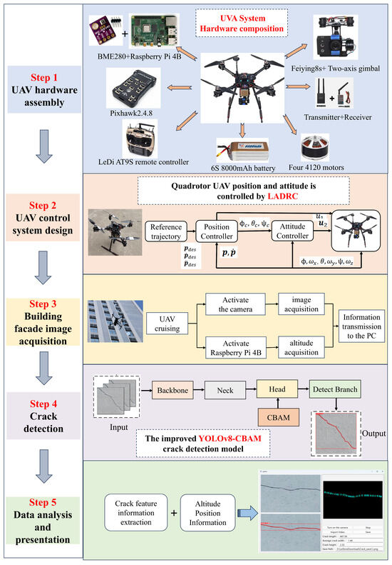
Figure 1.
Overall system configuration. It includes five parts: hardware composition, UAV control system design, exterior wall crack image acquisition, crack detection, data analysis, and interface display, as shown on the right.
The overall software flowchart of the crack detection UAV system proposed in this paper is shown in Figure 2. The system initialization process begins with the activation of the drone platform, followed by the startup of the camera, which transmits video via the 5.8 GHz RF wireless link. Simultaneously, the BME280 sensor is initialized through the I2C interface, and data is transmitted using the TCP/IP socket protocol. The PC receives the image stream and sensor data, performs crack detection based on YOLOv8-CBAM, and displays the results through the user interface.
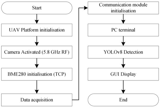
Figure 2.
The overall software interaction process.
2.1. System Modeling and Control System Design
The building crack detection UAV system employs a quadrotor UAV for aerial photography in densely built environments, which are characterized by a symmetric rigid body structure, uniform mass distribution, structural stability, and robust flight capability [38].
This study designs the control system based on dynamic modeling. The control rigid body motion model of the quadrotor UAV is as follows [39]:
where p is position, v is velocity, is Euler angles, is angular velocity, is the transformation matrix between and , g is gravitational acceleration, points in the z-axis direction of the Earth coordinate system, F is thrust, m is the mass of the UAV, is the rotation matrix, is the moment of inertia, is the torque, and are unknown disturbances, including aerodynamic drag, wind disturbance, time-varying loads, gyroscopic effects, etc. The dynamic model of the quadcopter UAV is as follows [40]:
where is the horizontal and vertical positions, where the first derivative is velocity, and the second derivative is acceleration, are the roll, pitch, and yaw angles, where the first derivative is angular velocity, and the second derivative is angular acceleration, is the control input, are rotational inertias about the three axes, are the rolling, pitching, and yawing moments generated by propellers along the body axis, is the drag coefficient, and are unknown disturbances, such as model parameter variations, gust disturbances, electromagnetic interference, strong airflows, etc.
The UAV control system adopts a position-attitude cascade closed-loop control framework [40]. The system structure is shown in Figure 3. The main control target is the position and attitude control of the UAV. The system input is a reference trajectory, including the desired position and the angle. The position controller compares the desired position with the current position feedback to generate the desired roll angle and pitch angle. The attitude controller then processes the attitude feedback from the position controller and calculates the desired control torque using the LADRC method. The innovation of LADRC lies in its introduction of the Disturbance Observer, which enables real-time estimation and compensation of system disturbances. This approach does not rely on an accurate system model and effectively suppresses unknown disturbances and nonlinear effects within the system. Specifically, the attitude controller incorporates a Linear Extended State Observer (LESO), with individual observers designed for each subsystem to estimate unmodeled dynamic disturbances in real time—such as aerodynamic forces, torques, and external interferences. Through pole placement, the closed-loop dynamic performance is precisely regulated [41], optimizing the observer’s dynamic response speed and stability, and performs dynamic compensation within the control law, thereby significantly enhancing the disturbance rejection capability and attitude stability of the UAV during flight [42]. These control signals are then distributed and converted into specific rotor speed commands, which drive the propulsion system of the UAV. The UAV dynamics model translates these rotor speeds into actual position and attitude, with these state variables being continuously fed back into the control loop.
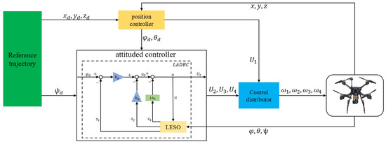
Figure 3.
Trajectory tracking control structure of UAV based on LADRC.
The mathematical formulations of the LADRC are presented as follows:
where and represent the estimated values of the state variables of the controlled object, while represents the real-time estimation of the external disturbance. Parameters , , and are the coefficients of the linear state observer, and and are the parameters of the LESO, u is the system control variable, is the intermediate control variable, and b is the controller gain, while is the controller compensation coefficient.
After bandwidth parameterization, the parameters are defined as
where and represent the state bandwidth and controller bandwidth, respectively [43]. Consequently, the parameter tuning task for LADRC is reduced to adjusting , , and , thereby significantly alleviating the complexity and effort involved in parameter configuration.
Among these parameters, the controller bandwidth critically determines the controller’s response speed. Within a predefined operational range, increasing generally enhances system control performance; however, excessively large values may provoke system instability. The observer bandwidth governs the tracking speed of the state observer. Elevated values enable faster estimation of external disturbances but may induce oscillatory behavior in the observer when excessively high. The control compensation coefficient characterizes the dynamic properties of the controlled object and is typically derived from the initial acceleration of the step response.
In this paper, the fundamental strategy for LADRC parameter tuning involves initially setting an appropriate controller bandwidth to ensure system stability, followed by a gradual increment of to improve the response speed. Upon encountering overshoot and instability, the observer bandwidth should be increased appropriately to mitigate overshoot, concurrently adjusting the ratio and the control compensation coefficient to strike an optimal balance between system responsiveness and stability. This iterative tuning process continues until satisfactory control performance is attained.
2.2. Acquisition of Building Facade Image and Altitude Information
Based on the stable flight of the UAV system, the system is equipped with a high-resolution camera and a Raspberry Pi 4B (Sony UK Technology Centre, Pencoed, UK ), enabling the UAV to fly to the target building for image acquisition. To meet the requirement of continuously capturing real-time imagery from building walls, the Falcon 8s was selected as the imaging device. This camera features a lightweight design with dimensions of mm, making it compact and lightweight, which enhances the flight performance and endurance of the UAV. It is equipped with a 12-megapixel IMX117 sensor, capable of capturing high-resolution images and 4 K video, allowing detailed visualization of the building’s exterior walls. Furthermore, the camera is mounted on a gimbal to ensure the stability of the camera and the clarity of the image during the flight, minimizing the effects of image blur and quality degradation caused by jitter.
Furthermore, to determine the altitude during the flight of the UAV, a BME280 sensor is connected to the Raspberry Pi 4B via the IIC interface. The BME280 sensor is a barometric sensor capable of measuring temperature, humidity, and air pressure [44]; the sampling frequency is 10–50 Hz. To reduce noise and improve signal stability, the raw barometric pressure data were smoothed using a moving average filter. It calculates altitude based on air pressure changes; the calculation formula is as follows:
where represents standard atmospheric pressure at sea level (typically 101,325 Pa), and P denotes the current atmospheric pressure.
2.3. Real-Time Wireless Data Transmission
After the data collection is completed, the system utilizes a transmitter and receiver for image data transmission. First, the UAV-mounted transmitter converts the captured video signals into digital images and transmits them to the receiver. Subsequently, the receiver processes the signals from the transmitter and converts them back into video signals and communicates based on the 5.8 GHz radio frequency band. Additionally, the height information of building cracks is transmitted to the PC terminal via the TCP protocol through the network communication module integrated in the Raspberry Pi.
2.4. Proposed YOLOv8-CBAM Crack Detection Algorithm
After receiving the data on the PC side, the detection task is performed. This system utilizes the proposed YOLOv8-CBAM model for building facade crack detection. YOLOv8 (You Only Look Once, Version 8), as the latest generation of object detection algorithms [45], combines the advantages of previous versions and employs a more efficient backbone network to extract richer features with lower computational cost [26]. Moreover, it abandons the traditional anchor-based mechanism and adopts an anchor-free design, simplifying both the training and inference processes, thus improving the model’s efficiency [46]. Additionally, the model integrates multi-scale feature fusion, ensuring high accuracy when detecting cracks of various sizes. However, when handling relatively complex crack detection tasks, the model may overlook fine or intricate features [47]. Small or low-contrast cracks may be missed due to background noise or significant texture variations, leading to false positives or missed detections. To address this issue, this study introduces the Convolutional Block Attention Module (CBAM) into the YOLOv8 base model, allowing the model to focus on important feature regions across both the channel and multi-scale dimensions. This enhances the sensitivity to detailed features while suppressing interference from irrelevant regions, ensuring that the model maintains high robustness and accuracy even in dense backgrounds and multi-crack environments.
Figure 4 illustrates the structure of the YOLOv8-CBAM model, which includes a backbone, neck, and head, with the CBAM integrated into the neck. The backbone consists of multiple convolutional layers (Conv) that extract both low-level and mid-level features from the input image. This part is pre-trained to generate feature maps from the input crack images, providing the depth information required for subsequent network processing [48]. The neck network, enhanced by CBAM, processes feature maps at different scales, integrating and optimizing features from various layers to facilitate crack detection in complex environments. The head network, consisting of fully connected or convolutional layers, is responsible for classifying targets, regressing bounding boxes, and predicting the confidence of cracks, providing the final output for object detection.
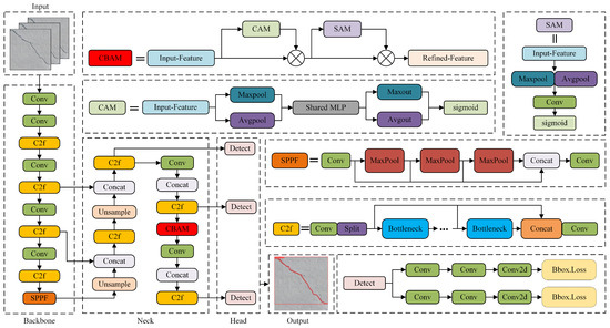
Figure 4.
The proposed YOLOv8-CBAM model structure diagram.
The CBAM is integrated into the multi-scale feature fusion process of the YOLOv8 architecture, effectively enhancing the discriminative capability of feature representations. By selectively emphasizing informative features in both the channel and spatial dimensions, the model is able to automatically focus on critical crack-related features. This mechanism suppresses irrelevant background noise and highlights fine-grained crack details, thereby significantly improving the robustness and accuracy of crack detection, particularly in complex real-world environments.
Figure 5 illustrates the detailed structure of the Channel Attention Module (CAM) and Spatial Attention Module(SAM) in the CBAM. The CAM utilizes the Squeeze-and-Excitation Module to adjust the channel weights of the feature map. This module compresses the feature map through global average pooling, and then generates the channel weights using two fully connected layers and activation functions [49]. Finally, the weights of each channel in the feature map are recalibrated by the multiplication of elements. The SAM uses the CBAM to adjust the spatial weights of the feature map. This module first generates two distinct feature maps through max pooling and average pooling, and then produces the spatial attention map using a convolutional layer. Ultimately, the spatial distribution of the feature map is recalibrated by element-wise multiplication.
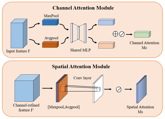
Figure 5.
The detailed structure of the CAM and SAM in the CBAM.
2.5. Crack Information Extraction
After segmenting and detecting wall cracks using a semantic segmentation network, the foreground image of the cracks is obtained. However, this image cannot be directly interpreted by a computer. Therefore, the segmented crack image undergoes secondary processing to extract the crack edge lines and the medial axis, which are subsequently used to calculate the crack length and average width. The overall process is illustrated in Figure 6.
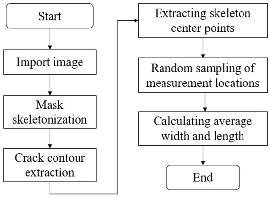
Figure 6.
Crack information extraction process.
Skeleton extraction, also known as binary image thinning, refines a connected region into a one-pixel-width structure, which is used for feature extraction and topological representation of the target. In this paper, the Skeletonize method is employed to perform skeleton extraction, where all pixels marked as skeleton points are extracted to form the final skeleton image. As shown in Figure 7.
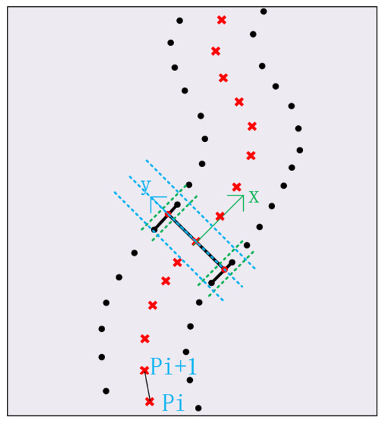
Figure 7.
Orthogonal skeleton line. (The black dots represent the boundaries of the cracks, and the red cross represent the centerlines).
The total length of the crack is estimated by calculating the distances between the skeleton points, as shown in the following equation:
where L represents the length of the crack, n is the number of skeleton points, and is the distance between adjacent skeleton points and .
The crack width is calculated using the orthogonal distance from each skeleton point to the edge. The width at each skeleton point is defined as the minimum distance from that point to the crack edge. The average crack width is obtained by taking the mean of the widths at all skeleton points. The calculation formula is as follows:
where represents the average width of the crack, is the orthogonal distance from the skeleton point to the crack boundary, and n is the number of skeleton points.
The calculation of crack length and width relies on the pixel-to-real-world conversion factor k, which was determined through a calibration experiment using a reference board. The conversion factor was established as , with a calibration standard deviation of . The primary source of error in length measurement stems from the localization of skeleton points, with an associated standard deviation of . The error in width estimation is mainly influenced by boundary detection uncertainty, with a mean deviation of . The final measurement uncertainty is expressed as .
3. Experiments
3.1. UAV Trajectory Tracking Experiment Based on LADRC
To verify the effectiveness of the proposed control algorithm, a trajectory tracking simulation experiment of the proposed LADRC control algorithm was conducted in the MATLAB 2021b simulation environment, and a comparative analysis was performed with the cascade PID controller. The system model parameters of the UAV in the simulation experiment are shown in Table 2. During the controller parameter design, tuning was carried out according to the parameter selection principles outlined in Section 2.1. After multiple trials, the final parameters for the Linear Active Disturbance Rejection Control (LADRC) and cascade PID controllers are presented in Table 3 and Table 4.
Table 2.
UAV simulation parameters.
Table 3.
LADRC parameters for UAV control.
Table 4.
PID parameters for UAV control.
First, the stability of LADRC in UAV attitude control is verified by conducting a trajectory tracking experiment using a complex time-varying trajectory. The initial position and attitude of the UAV are set as , and the desired trajectory for tracking is set as . The simulation results are shown in Figure 8, Figure 9, Figure 10 and Figure 11, which represent the trajectory tracking in the x, y, and z directions, as well as in three dimensions.
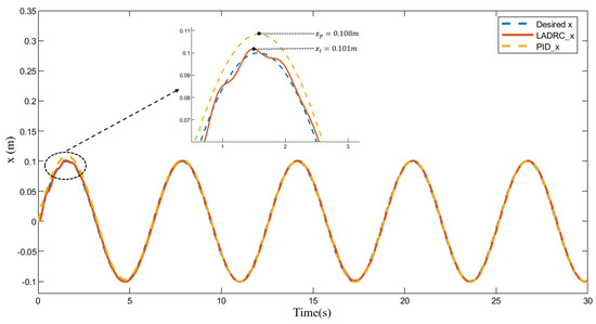
Figure 8.
x-direction trajectory tracking results.
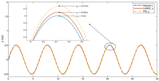
Figure 9.
y-direction trajectory tracking results.
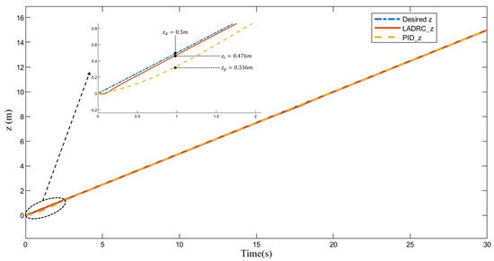
Figure 10.
z-direction trajectory tracking results.
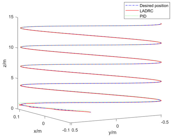
Figure 11.
3D trajectory tracking results.
As shown in Figure 8, the tracking error under PID controller is m, while the tracking error under the proposed LADRC controller is 0.001 m. Clearly, the maximum error of the proposed LADRC is smaller. Figure 9 shows that during the approximately straight-line flight phase of the UAV, the tracking performance of both controllers is similar. However, at the trajectory switching point, the tracking error of the PID controller is about 0.15 m, while the tracking error of the LADRC controller is only m. As shown in Figure 10, both PID and LADRC controllers perform well in tracking the desired trajectory along the z-axis, with little difference between the two. Figure 11 further demonstrates that during the turning phase in the takeoff stage, trajectory tracking error under the action of the LADRC controller is significantly smaller than that of the PID controller, exhibiting better performance.
The above experiment verified the flight performance of the UAV under non-interfered conditions, representing the ideal experimental scenario. However, in practical flight scenarios, natural wind disturbances are inevitable environmental factors. To verify the robustness of the designed controller under external disturbance conditions, this experiment introduces a wind disturbance model into the system and conducts comparative analysis with PID and LADRC controllers. Specifically, a stochastic function with frequency modulation, , is introduced in the x-direction to simulate the randomness of natural wind, while a segment function is applied in the y-direction to emulate burst wind disturbances. The calculation formulas for , , and the simulated wind force are as follows:
The meanings and numerical values of the parameters in Equations (7)–(9) are listed in Table 5.
Table 5.
Simulation wind field parameters and their definitions.
In this experiment, the wind disturbance in the x-direction is applied during , while the wind disturbance in the y-direction occurs during . Figure 12 and Figure 13 illustrate the magnitude and duration of the simulated wind. Figure 14 and Figure 15 present the trajectory responses in the x and y-directions under wind disturbances, as well as the variation of UAV attitude angles induced by the disturbances.
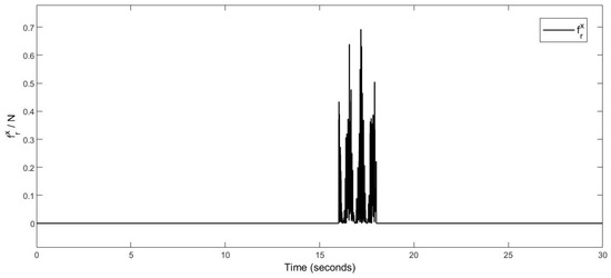
Figure 12.
Simulated wind magnitude and duration in the x-direction.
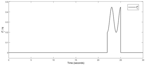
Figure 13.
Simulated wind magnitude and duration in the y-direction.
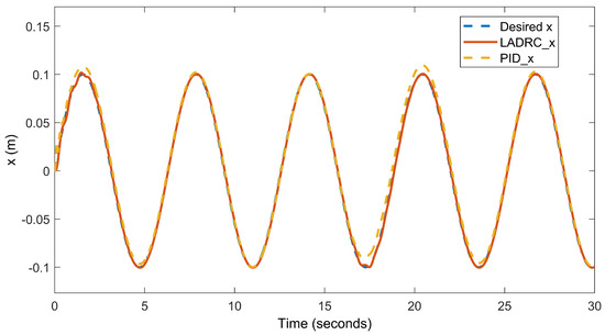
Figure 14.
x-direction trajectory tracking results under wind disturbances.
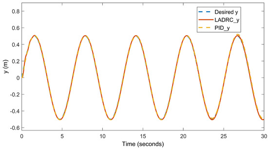
Figure 15.
y-direction trajectory tracking results under wind disturbances.
The simulation results indicate that both controllers can respond to wind disturbances; however, in terms of disturbance suppression, the LADRC controller exhibits superior performance. Whether considering the maximum deviation during the disturbance or the recovery time required for the trajectory to return to the desired path after the disturbance, LADRC consistently outperforms the PID controller. Taking the x-direction as an example, the robustness comparison results of each controller under wind disturbances are presented in Table 6.
Table 6.
Robustness comparison of two controllers under wind disturbance conditions (in the x-direction). (The best data is bolded).
As shown in Table 6, the maximum disturbance deviation of the LADRC controller is only 0.001 m, which is 0.01 m less than that of the PID controller. In terms of recovery time, LADRC requires only 0.4 s, a reduction of 6.33 s compared to PID. To further visualize the robustness of the controllers during disturbance events, the error response curves of the x and y channels are plotted. As illustrated in Figure 16 and Figure 17, the LADRC controller demonstrates a stronger disturbance rejection capability.
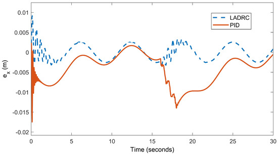
Figure 16.
The error response curves of the x-directions.
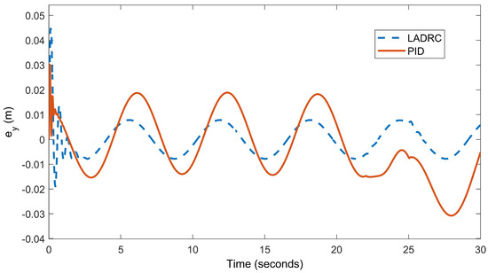
Figure 17.
The error response curves of the y-directions.
3.2. Crack Detection Experiment Based on Improved YOLOv8-CBAM
This paper uses , , and - to evaluate the performance of the proposed YOLOv8-CBAM model in crack detection tasks. By evaluating the inference on the dataset and comparing the predicted results with the ground truth labels [50], the calculation formulas are as follows:
where represents the number of correctly detected cracks, denotes the number of cracks incorrectly identified as positive, and refers to the number of missed cracks. measures the accuracy of positive predictions, evaluates the detection rate of positive samples, and the F1-score is the harmonic mean of both [51].
Additionally, for crack object detection, - () and () are used as key performance metrics; the calculation formulas are as follows:
where represents the area under the precision–recall curve for a single class, while is the mean of the across all classes. P and R denote precision and recall, respectively, with representing precision at a specific recall rate, and N being the total number of classes. Additionally, to evaluate detection quality, Intersection over Union (IoU) is used to quantify the overlap between the predicted bounding box and the ground truth bounding box. When the IoU exceeds a predefined threshold, the detection result is considered valid; otherwise, it is deemed invalid.
The model training in this study was conducted using the equipment listed in Table 7.
Table 7.
Software and hardware version models.
To evaluate the accuracy of the crack detection algorithm proposed in this paper, we utilized the publicly available Crack Segmentation Detection (CSD) dataset from Roboflow. This dataset contains cracks of varying severity on different types of concrete surfaces. An example image from the dataset is shown in Figure 18. The dataset consists of 2663 crack images, each with a resolution of 640 × 640 pixels. The dataset is divided into a training set of 2326 images, a validation set of 225 images, and a test set of 112 images. Additionally, the YOLOv8-CBAM model proposed in this study was trained using the hyperparameters specified in Table 8.
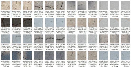
Figure 18.
Sample crack images from the CSD dataset.
Table 8.
Hyperparameters for YOLOv8-CBAM model training.
In detection performance, Figure 19a shows that precision approaches as confidence increases, indicating a low false positive rate of the model. Figure 19b BoxPR illustrates the precision–recall curve, with mAP@0.5 reaching 0.974, demonstrating a good balance between precision and recall. Figure 19c indicates that the F1-score reaches its optimal value of 0.97 at a confidence level of 0.575, reflecting the best model performance at this threshold. Figure 19d shows that the recall decreases slightly at higher confidence levels but generally maintains a high level, indicating a strong detection capability. In the segmentation task, Figure 20a shows that the precision is close to 1 at high confidence, reflecting a low false positive rate in segmentation. Figure 20b shows that the recall increases as confidence decreases, highlighting the strong coverage ability of the model. Figure 20c demonstrates that the best F1-score of 0.97 occurs at a confidence level of 0.575, indicating the optimal segmentation performance. Figure 20d shows that the model achieves an mAP@0.5 of 0.974, further proving that it balances high precision and high recall in segmentation tasks. In conclusion, the proposed YOLOv8-CBAM model demonstrates excellent performance in crack detection and segmentation tasks, effectively balancing precision and recall, and is suitable for complex crack detection scenarios.
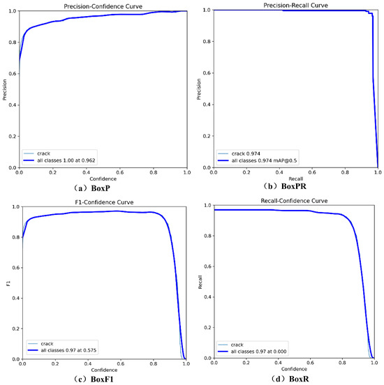
Figure 19.
Performance diagnostic curves for detection frames (the top-left is the precision–confidence curve, the top-right is the precision–recall curve, the bottom-left is the F1–confidence curve, and the bottom-right is the recall–confidence curve).
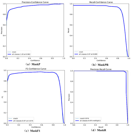
Figure 20.
Performance diagnostic curves for image segmentation (the top-left is the precision–confidence curve, the top-right is the precision–recall curve, the bottom-left is the F1–confidence curve, and the bottom-right is the recall–confidence curve).
To validate the effectiveness and high applicability of the YOLOv8-CBAM proposed in this paper for crack detection scenarios, we incorporated two other attention mechanisms, SE (Squeeze-and-Excitation) and ECA (Efficient Channel Attention), into the YOLOv8 model for comparison. A comparative analysis is then conducted against the original YOLOv8-seg model using the testing dataset. In the object detection task, as shown in Table 9, YOLOv8-CBAM demonstrates outstanding performance in terms of Box Precision (96.2%) and Box Recall (97.0%), with an mAP50-95 of 91.73% and a Box loss of 0.39171, outperforming YOLOv8-SE and YOLOv8-ECA. This highlights its superior detection performance and robustness. Although YOLOv8l-seg and YOLOv8x-seg achieve a higher mAP50 of 97.2%, YOLOv8-CBAM exhibits a more lightweight model structure, achieving an mAP50-95 of 91.73% and striking a better balance between model complexity and robustness. In the instance segmentation task, as presented in Table 10, YOLOv8-CBAM maintains high mask precision (97%) and recall (97.9%), with its mAP50 (98.4%) and mAP50-95 (54.77%) surpassing the other six models, indicating the significant advantage of the CBAM module in segmentation accuracy and generalization capability. Regarding computational efficiency, as shown in Table 11, YOLOv8-CBAM delivers excellent performance with 11.7 M parameters and a file size of 15.1 MB, achieving an inference time of only 7.6 ms, which is lower than YOLOv8-SE and YOLOv8-ECA, second only to YOLOv8s-seg. This demonstrates its faster computation speed and lower hardware requirements. Therefore, YOLOv8-CBAM, while maintaining high accuracy, offers a more lightweight model structure and higher computational efficiency, making it suitable for real-time applications in resource-constrained environments, fully proving its advantages in practical crack detection applications.
Table 9.
Performance comparison of different model detection frames based on the test set (the best data is bolded).
Table 10.
Performance comparison of different model segmentation based on the test set (the best data is bolded).
Table 11.
Comparison of different model parameters (the best data is bolded).
Figure 21 illustrates the training and validation process of the proposed YOLOv8-CBAM model in the object detection task. The model’s convergence and generalization ability are assessed by tracking changes in the loss functions and performance metrics. During the training phase, the -, -, -, and - all significantly decreased as the number of training epochs increased. For example, - dropped from an initial value of approximately 3.0 to below 0.5, indicating good convergence in bounding box selection, segmentation, classification, and distribution focal loss optimization. Regarding performance metrics, (B) and (B) gradually approached 1, while /(M) and (M) continuously increased, ultimately reaching values above 0.9. In the validation phase, loss functions such as - and - showed significant fluctuations in the early stages but gradually decreased and stabilized, with - dropping from an initial value of around 3.0 to below 1.0. This demonstrates the stability and generalization capability of the proposed YOLOv8-CBAM model. Additionally, performance metrics such as 50 and 50-95 steadily improved during the validation phase, with 50(M) exceeding 0.9, indicating the overall superior performance of the model in the object detection task.
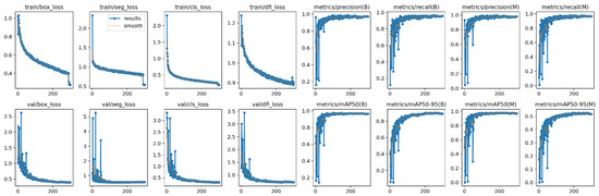
Figure 21.
The loss and performance metric variation curves of the YOLOv8-CBAM model during training and validation (the horizontal axis represents the training epochs, and the vertical axis represents various metrics such as loss values, precision, recall, and mAP).
Figure 22 shows the performance of the five models in crack detection. The YOLOv8-CBAM model performs well in detecting fine cracks and handling complex backgrounds. Its detection lines are more continuous and precise in Figure 22a,f,k,p. YOLOv8s-seg performs moderately well in simple scenes such as subfigure b, but suffers from detection discontinuities or inaccurate boundaries in complex scenes (Figure 22g,l), as well as leakage detection (Figure 22q). As for YOLOv8x-seg, although it provides relatively continuous detection in some aspects, it also suffers from misdetection (Figure 22j) and insufficient detail capture (Figure 22t).
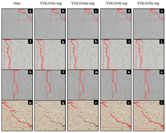
Figure 22.
The performance of the five models in crack detection (the red box is the detection box, and the red curve represents the detected cracks, (a–t) represent the crack detection conditions).
Overall, the proposed YOLOv8-CBAM model proposed in this paper exhibits good convergence during training and strong generalization capability and detection accuracy during the validation phase, validating the effectiveness of the proposed model optimization.
3.3. Real-World Experiment
To verify the practical feasibility of the building crack detection UAV system for detecting cracks in building exterior walls, we carried out a crack detection experiment in a high-rise residential area. This area is well lit and often has gentle breezes, providing an ideal environment for system testing, as shown in Figure 23. This system adopts the Yuanhang ZD550 quadcopter UAV platform (Yuanhang technology, Kaiping, Guangdong, China), is equipped with a lithium battery with a battery capacity of 111 Wh, and is configured with various auxiliary devices, including Raspberry Pi 4B, Feiying 8s camera, and a BME280 sensor and wireless transmission module. The total power consumption of the auxiliary devices is approximately 10.51 W. The measured data shows that the power consumption of the motor in the hovering state is approximately 150 W. Combined with the auxiliary equipment, the total system power consumption is approximately 160.51 W. Based on the calculation results of the battery capacity and power consumption of the system, the theoretical hovering endurance time is approximately 0.69 h, which is approximately 41 min. Endurance capacity, as a key indicator of continuous inspection tasks, is limited by battery capacity and the overall energy consumption level, and it is an important factor that needs to be weighed urgently in the actual deployment of this system. The actual flight tests are as follows:
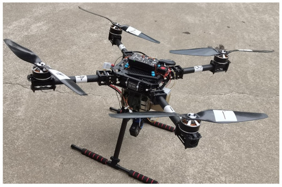
Figure 23.
UAV hardware integration.
Tests indicate that (Table 12), under a fully charged battery, the system can perform effective inspection tasks for 35–40 min. Flight duration is significantly affected by environmental factors such as wind speed, temperature, and mission mode; strong winds or low temperatures may reduce flight time to around 30 min. In addition, the Raspberry Pi 4B operates with a CPU utilization ranging about . The ground station maintains a processing frame rate of 20 to 30 FPS, supporting efficient inference. The overall end-to-end latency remains below 800 ms, which meets the real-time monitoring requirements to detect cracks on the exterior walls of buildings.
Table 12.
Power consumption and flight duration under different flight modes.
The UAV performs cruising and captures video data, which is then transmitted to the ground station for detection. After the detection is completed, the crack data is analyzed, and the interface is visualized. As shown in Figure 24, Figure 25 and Figure 26, the top-left corner displays the raw data received by the PC from the UAV camera, while the bottom-left corner shows the crack detection and annotation using the improved YOLOv8 model. The right side presents the crack skeleton feature extraction and crack feature information, including the current UAV altitude, crack length, and average width. Furthermore, Table 13 presents a quantitative evaluation of the proposed segmentation model on three selected real-world crack images, using three key metrics: Box Intersection over Union (Box IoU), Mask Intersection over Union (Mask IoU), and Pixel Accuracy (PA). The Box IoU ranges from 84.5% to 88.23%, indicating accurate object-level bounding performance. The Mask IoU, which reflects the pixel-level segmentation quality, ranges from 86.85% to 96.33%, demonstrating effective boundary delineation of crack regions. Additionally, the pixel accuracy for all samples remains above 98.9%, with a peak value of 99.73%, highlighting the robustness of the model in maintaining fine-grained pixel classification. These results confirm that the model not only detects crack regions accurately at the object level but also achieves high-fidelity segmentation at the pixel level. The real-world experiment has been verified.
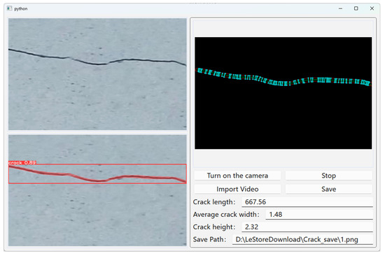
Figure 24.
Crack 1 detection interface (the top-left is the original image, the bottom-left is crack detection and annotation, and the right side is crack skeleton feature extraction and crack feature information).
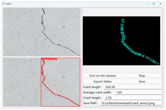
Figure 25.
Crack 2 detection interface (the top-left is the original image, the bottom-left is crack detection and annotation, and the right side is crack skeleton feature extraction and crack feature information).
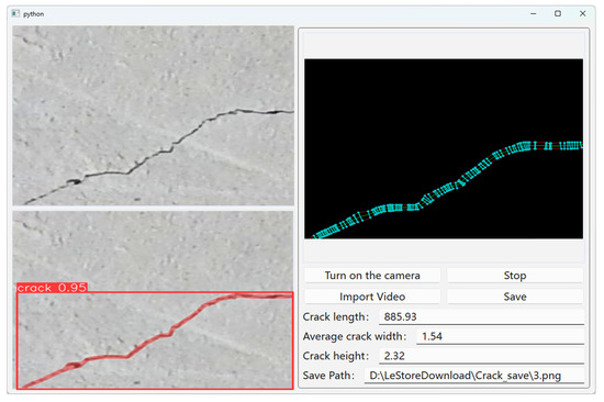
Figure 26.
Crack 3 detection interface (the top-left is the original image, the bottom-left is crack detection and annotation, and the right side is crack skeleton feature extraction and crack feature information).
Table 13.
Three types of crack detection interfaces are displayed.
4. Conclusions and Future Research
This paper presents a building crack detection UAV system based on the improved YOLOv8 algorithm, designed for detecting cracks in the exterior walls of buildings. By leveraging the flexibility of UAVs and their aerial perspective, the system enables efficient data collection from the exterior walls and real-time transmission to a ground station. The integration of the improved LADRC ensures safe and stable UAV flight under high-rise disturbances, further enhancing the effectiveness of image capture. Additionally, the improved YOLOv8 model effectively achieves accurate and robust crack detection in complex backgrounds and crack environments. Extensive field experiments validate that the system can perform high-precision crack detection and analysis of buildings even in challenging disturbed environments.
Future work will focus on the adoption of multi-sensor data fusion and achieving real-time autonomous flight for UAVs.
Author Contributions
Conceptualization, L.Z. and L.G.; methodology, L.G., L.W., and Z.W.; software, L.W. and Z.W.; validation, L.Z. and L.G.; investigation, L.W. and Z.W.; writing—original draft preparation, L.G. and L.Z.; writing—review and editing, L.G. and L.Z.; visualization, Z.W.; supervision, S.Y. All authors have read and agreed to the published version of the manuscript.
Funding
This research was funded, in part, by the Yulin Science and Technology Research Program (2023-CXY-184) and, in part, by the Xi’an Science and Technology Research Program (24GXFW0023). This support is gratefully acknowledged.
Data Availability Statement
Dataset available on request from the authors.
Acknowledgments
All authors thank the editors and anonymous reviewers for their critical comments and suggestions for improving the manuscript.
Conflicts of Interest
The authors declare no conflicts of interest.
Abbreviations
The following abbreviations are used in this manuscript:
| YOLO | You Only Look Once |
| LADRC | Linear Active Disturbance Rejection Control |
| CAM | Channel Attention Module |
| SAM | Spatial Attention Module |
| CBAM | Convolutional Block Attention Module |
| SNR | Signal-to-Noise Ratio |
| CNN | Convolutional Neural Networks |
References
- Jiang, Y.; Han, S.; Bai, Y. Building and infrastructure defect detection and visualization using drone and deep learning technologies. J. Perform. Constr. Facil. 2021, 35, 04021092. [Google Scholar] [CrossRef]
- Zhang, R.; Li, H.; Duan, K.; You, S.; Liu, K.; Wang, F.; Hu, Y. Automatic detection of earthquake-damaged buildings by integrating UAV oblique photography and infrared thermal imaging. Remote Sens. 2020, 12, 2621. [Google Scholar] [CrossRef]
- Mutlib, N.K.; Baharom, S.B.; El-Shafie, A.; Nuawi, M.Z. Ultrasonic health monitoring in structural engineering: Buildings and bridges. Struct. Control Health Monit. 2016, 23, 409–422. [Google Scholar] [CrossRef]
- Berrocal, C.G.; Fernandez, I.; Rempling, R. Crack monitoring in reinforced concrete beams by distributed optical fiber sensors. Struct. Infrastruct. Eng. 2021, 17, 124–139. [Google Scholar] [CrossRef]
- Oliveira, H.; Correia, P.L. Automatic road crack detection and characterization. IEEE Trans. Intell. Transp. Syst. 2012, 14, 155–168. [Google Scholar] [CrossRef]
- Chen, Q.; Huang, Y.; Weng, X.; Liu, W. Curve-based crack detection using crack information gain. Struct. Control Health Monit. 2021, 28, e2764. [Google Scholar] [CrossRef]
- Yao, Y.; Tung, S.T.E.; Glisic, B. Crack detection and characterization techniques—An overview. Struct. Control Health Monit. 2014, 21, 1387–1413. [Google Scholar] [CrossRef]
- Liu, J.; Yang, X.; Lau, S.; Wang, X.; Luo, S.; Lee, V.C.S.; Ding, L. Automated pavement crack detection and segmentation based on two-step convolutional neural network. Comput.-Aided Civ. Infrastruct. Eng. 2020, 35, 1291–1305. [Google Scholar] [CrossRef]
- Talab, A.M.A.; Huang, Z.; Xi, F.; HaiMing, L. Detection crack in image using Otsu method and multiple filtering in image processing techniques. Optik 2016, 127, 1030–1033. [Google Scholar] [CrossRef]
- Ashraf, A.; Sophian, A.; Shafie, A.A.; Gunawan, T.S.; Ismail, N.N.; Bawono, A.A. Efficient Pavement Crack Detection and Classification Using Custom YOLOv7 Model. Indones. J. Electr. Eng. Inform. (IJEEI) 2023, 11, 119–132. [Google Scholar] [CrossRef]
- Akagic, A.; Buza, E.; Omanovic, S.; Karabegovic, A. Pavement crack detection using Otsu thresholding for image segmentation. In Proceedings of the 2018 41st International Convention on Information and Communication Technology, Electronics and Microelectronics (MIPRO), Opatija, Croatia, 21–25 May 2018; pp. 1092–1097. [Google Scholar] [CrossRef]
- Wang, Y.; Zhang, J.Y.; Liu, J.X.; Zhang, Y.; Chen, Z.P.; Li, C.G.; He, K.; Yan, R.B. Research on crack detection algorithm of the concrete bridge based on image processing. Procedia Comput. Sci. 2019, 154, 610–616. [Google Scholar] [CrossRef]
- Ying, L.; Salari, E. Beamlet transform-based technique for pavement crack detection and classification. Comput.-Aided Civ. Infrastruct. Eng. 2010, 25, 572–580. [Google Scholar] [CrossRef]
- Kim, H.; Ahn, E.; Shin, M.; Sim, S.H. Crack and noncrack classification from concrete surface images using machine learning. Struct. Health Monit. 2019, 18, 725–738. [Google Scholar] [CrossRef]
- Hsieh, Y.A.; Tsai, Y.J. Machine learning for crack detection: Review and model performance comparison. J. Comput. Civ. Eng. 2020, 34, 04020038. [Google Scholar] [CrossRef]
- Zhang, L.; Shen, J.; Zhu, B. A research on an improved Unet-based concrete crack detection algorithm. Struct. Health Monit. 2021, 20, 1864–1879. [Google Scholar] [CrossRef]
- Tran, T.S.; Nguyen, S.D.; Lee, H.J.; Tran, V.P. Advanced crack detection and segmentation on bridge decks using deep learning. Constr. Build. Mater. 2023, 400, 132839. [Google Scholar] [CrossRef]
- Chen, P.H.; Shen, H.K.; Lei, C.Y.; Chang, L.M. Support-vector-machine-based method for automated steel bridge rust assessment. Autom. Constr. 2012, 23, 9–19. [Google Scholar] [CrossRef]
- Tran, T.T.; Ozer, E. Automated and model-free bridge damage indicators with simultaneous multiparameter modal anomaly detection. Sensors 2020, 20, 4752. [Google Scholar] [CrossRef]
- Malekjafarian, A.; Golpayegani, F.; Moloney, C.; Clarke, S. A machine learning approach to bridge-damage detection using responses measured on a passing vehicle. Sensors 2019, 19, 4035. [Google Scholar] [CrossRef]
- Sun, S.; Liang, L.; Li, M.; Li, X. Vibration-based damage detection in bridges via machine learning. KSCE J. Civ. Eng. 2018, 22, 5123–5132. [Google Scholar] [CrossRef]
- Zhang, L.; Yang, F.; Zhang, Y.D.; Zhu, Y.J. Road crack detection using deep convolutional neural network. In Proceedings of the 2016 IEEE International Conference on Image Processing (ICIP), Phoenix, AZ, USA, 25–28 September 2016; pp. 3708–3712. [Google Scholar] [CrossRef]
- Zou, Q.; Zhang, Z.; Li, Q.; Qi, X.; Wang, Q.; Wang, S. Deepcrack: Learning hierarchical convolutional features for crack detection. IEEE Trans. Image Process. 2018, 28, 1498–1512. [Google Scholar] [CrossRef]
- Guo, J.M.; Markoni, H.; Lee, J.D. BARNet: Boundary aware refinement network for crack detection. IEEE Trans. Intell. Transp. Syst. 2021, 23, 7343–7358. [Google Scholar] [CrossRef]
- Cui, X.; Wang, Q.; Dai, J.; Zhang, R.; Li, S. Intelligent recognition of erosion damage to concrete based on improved YOLO-v3. Mater. Lett. 2021, 302, 130363. [Google Scholar] [CrossRef]
- Xiong, C.; Zayed, T.; Abdelkader, E.M. A novel YOLOv8-GAM-Wise-IoU model for automated detection of bridge surface cracks. Constr. Build. Mater. 2024, 414, 135025. [Google Scholar] [CrossRef]
- Joshi, D.; Singh, T.P.; Sharma, G. Automatic surface crack detection using segmentation-based deep-learning approach. Eng. Fract. Mech. 2022, 268, 108467. [Google Scholar] [CrossRef]
- Lei, B.; Ren, Y.; Wang, N.; Huo, L.; Song, G. Design of a new low-cost unmanned aerial vehicle and vision-based concrete crack inspection method. Struct. Health Monit. 2020, 19, 1871–1883. [Google Scholar] [CrossRef]
- Forcael, E.; Román, O.; Stuardo, H.; Herrera, R.F.; Soto-Muñoz, J. Evaluation of Fissures and Cracks in Bridges by Applying Digital Image Capture Techniques Using an Unmanned Aerial Vehicle. Drones 2023, 8, 8. [Google Scholar] [CrossRef]
- Rosales, C.; Tosetti, S.; Soria, C.; Rossomando, F. Neural adaptive PID control of a quadrotor using EFK. IEEE Lat. Am. Trans. 2018, 16, 2722–2730. [Google Scholar] [CrossRef]
- Mofid, O.; Mobayen, S.; Wong, W.K. Adaptive terminal sliding mode control for attitude and position tracking control of quadrotor UAVs in the existence of external disturbance. IEEE Access 2020, 9, 3428–3440. [Google Scholar] [CrossRef]
- Moreno-Valenzuela, J.; Pérez-Alcocer, R.; Guerrero-Medina, M.; Dzul, A. Nonlinear PID-type controller for quadrotor trajectory tracking. IEEE/ASME Trans. Mechatronics 2018, 23, 2436–2447. [Google Scholar] [CrossRef]
- Lopez-Sanchez, I.; Moreno-Valenzuela, J. PID control of quadrotor UAVs: A survey. Annu. Rev. Control 2023, 56, 100900. [Google Scholar] [CrossRef]
- Alonge, F.; D’Ippolito, F.; Fagiolini, A.; Garraffa, G.; Sferlazza, A. Trajectory robust control of autonomous quadcopters based on model decoupling and disturbance estimation. Int. J. Adv. Robot. Syst. 2021, 18. [Google Scholar] [CrossRef]
- Thanh, H.L.N.N.; Huynh, T.T.; Vu, M.T.; Mung, N.X.; Phi, N.N.; Hong, S.K.; Vu, T.N.L. Quadcopter UAVs Extended States/Disturbance Observer-Based Nonlinear Robust Backstepping Control. Sensors 2022, 22, 5082. [Google Scholar] [CrossRef]
- Lin, P.; Wu, Z.; Fei, Z.; Sun, X.M. A generalized PID interpretation for high-order LADRC and cascade LADRC for servo systems. IEEE Trans. Ind. Electron. 2021, 69, 5207–5214. [Google Scholar] [CrossRef]
- Song, J.; Hu, Y.; Su, J.; Zhao, M.; Ai, S. Fractional-order linear active disturbance rejection control design and optimization based improved sparrow search algorithm for quadrotor UAV with system uncertainties and external disturbance. Drones 2022, 6, 229. [Google Scholar] [CrossRef]
- Pounds, P.; Mahony, R.; Corke, P. Modelling and control of a large quadrotor robot. Control Eng. Pract. 2010, 18, 691–699. [Google Scholar] [CrossRef]
- Ji, R.; Ma, J. Mathematical modeling and analysis of a quadrotor with tilting propellers. In Proceedings of the 2018 37th Chinese Control Conference (CCC), Wuhan, China, 25–27 July 2018; Volume 13, pp. 1718–1722. [Google Scholar] [CrossRef]
- Rinaldi, M.; Primatesta, S.; Guglieri, G. A comparative study for control of quadrotor UAVs. Appl. Sci. 2023, 13, 3464. [Google Scholar] [CrossRef]
- Qiao, Z.; Zhu, G.; Zhao, T. Quadrotor Cascade Control System Design Based on Linear Active Disturbance Rejection Control. Appl. Sci. 2023, 13, 6904. [Google Scholar] [CrossRef]
- Zhou, R.; Tan, W. Analysis and tuning of general linear active disturbance rejection controllers. IEEE Trans. Ind. Electron. 2018, 66, 5497–5507. [Google Scholar] [CrossRef]
- Zhou, H. Design and Implementation of Intelligent Car Control System Based on Android System and Raspberry Pi. In Proceedings of the 2024 3rd International Conference on Electronics and Information Technology (EIT), Chengdu, China, 20–22 September 2024; pp. 457–462. [Google Scholar] [CrossRef]
- Wibawa, I.M.S.; Putra, I.K. Design of Air Pressure and Height Measuring Equipment Based on Arduino Nano Using BME280 Sensor. Int. Res. J. Eng. IT Sci. Res. 2022, 8, 222–229. [Google Scholar] [CrossRef]
- Cao, Y.; Pang, D.; Zhao, Q.; Yan, Y.; Jiang, Y.; Tian, C.; Wang, F.; Li, J. Improved yolov8-gd deep learning model for defect detection in electroluminescence images of solar photovoltaic modules. Eng. Appl. Artif. Intell. 2024, 131, 107866. [Google Scholar] [CrossRef]
- Wang, G.; Chen, Y.; An, P.; Hong, H.; Hu, J.; Huang, T. UAV-YOLOv8: A small-object-detection model based on improved YOLOv8 for UAV aerial photography scenarios. Sensors 2023, 23, 7190. [Google Scholar] [CrossRef] [PubMed]
- Wang, X.; Gao, H.; Jia, Z.; Li, Z. BL-YOLOv8: An improved road defect detection model based on YOLOv8. Sensors 2023, 23, 8361. [Google Scholar] [CrossRef] [PubMed]
- Yang, G.; Wang, J.; Nie, Z.; Yang, H.; Yu, S. A lightweight YOLOv8 tomato detection algorithm combining feature enhancement and attention. Agronomy 2023, 13, 1824. [Google Scholar] [CrossRef]
- Li, Y.; Li, Q.; Pan, J.; Zhou, Y.; Zhu, H.; Wei, H.; Liu, C. Sod-yolo: Small-object-detection algorithm based on improved yolov8 for UAV images. Remote Sens. 2024, 16, 3057. [Google Scholar] [CrossRef]
- Tang, J.; Feng, A.; Korkhov, V.; Pu, Y. Enhancing Road Crack Detection Accuracy with BsS-YOLO: Optimizing Feature Fusion and Attention Mechanisms. arXiv 2024, arXiv:2412.10902. [Google Scholar] [CrossRef]
- Zheng, X.; Mo, J.; Wang, S. DFL-YOLO: A tunnel crack detection algorithm for feature aggregation in complex scenarios. In Proceedings of the Fourth International Conference on Advanced Algorithms and Neural Networks (AANN 2024), Qingdao, China, 9–11 August 2024; Volume 13416, pp. 229–233. [Google Scholar] [CrossRef]
Disclaimer/Publisher’s Note: The statements, opinions and data contained in all publications are solely those of the individual author(s) and contributor(s) and not of MDPI and/or the editor(s). MDPI and/or the editor(s) disclaim responsibility for any injury to people or property resulting from any ideas, methods, instructions or products referred to in the content. |
© 2025 by the authors. Licensee MDPI, Basel, Switzerland. This article is an open access article distributed under the terms and conditions of the Creative Commons Attribution (CC BY) license (https://creativecommons.org/licenses/by/4.0/).