Deep-CNN-Based Layout-to-SEM Image Reconstruction with Conformal Uncertainty Calibration for Nanoimprint Lithography in Semiconductor Manufacturing

Abstract

Nanoimprint lithography (NIL) has emerged as a promising sub-10 nm patterning at low cost; yet, robust process control remains difficult because of time-consuming physics-based simulators and labeled SEM data scarcity. We propose a data-efficient, two-stage deep-learning framework here that directly reconstructs post-imprint SEM images from binary design layouts and delivers calibrated pixel-by-pixel uncertainty simultaneously. First, a shallow U-Net is trained on conformalized quantile regression (CQR) to output 90% prediction intervals with statistically guaranteed coverage. Moreover, per-level errors on a small calibration dataset are designed to drive an outlier-weighted and encoder-frozen transfer fine-tuning phase that refines only the decoder, with its capacity explicitly focused on regions of spatial uncertainty. On independent test layouts, our proposed fine-tuned model significantly reduces the mean absolute error (MAE) from 0.0365 to 0.0255 and raises the coverage from 0.904 to 0.926, while cutting the labeled data and GPU time by 80% and 72%, respectively. The resultant uncertainty maps highlight spatial regions associated with error hotspots and support defect-aware optical proximity correction (OPC) with fewer guard-band iterations. Extending the current perspective beyond OPC, the innovatively model-agnostic and modular design of the pipeline here allows flexible integration into other critical stages of the semiconductor manufacturing workflow, such as imprinting, etching, and inspection. In these stages, such predictions are critical for achieving higher precision, efficiency, and overall process robustness in semiconductor manufacturing, which is the ultimate motivation of this study.

1. Introduction

1.1. Nanoimprint Lithography: Principles, Advantages, and Manufacturing Challenges

Nanoimprint lithography (NIL) has emerged as an inspiring replacement for conventional photolithography recently, with a low-cost and high-resolution patterning process for sub-10 nm nodes [1,2,3]. The simplicity of its process flow—comprising master template creation and replica template fabrication, and final wafer patterning—makes it particularly suitable for high-throughput manufacturing [4]. In contrast to conventional optical lithography, which relies on the use of reduction masks (typically 4× or 5×), NIL makes use of a 1:1 imprint template to pattern the substrate directly at the nanoscale. This one-to-one transfer mechanism reduces the reliance on traditional optical proximity correction (OPC), which compensates for distortions introduced by optical systems. While OPC plays a vital role in ensuring that the pattern on the wafer is identical to the design layout, its models are based on the physics of optical lithography. NIL, on the other hand, relies on entirely different mechanisms such as mechanical contact and polymer flow, which calls for new OPC frameworks specific to imprint-based techniques. To ensure pattern fidelity, OPC often employs guard bands—conservative layout margins that require costly iterative tuning, which NIL’s distinct physics now demand to be redefined. The strategic importance of NIL has been increasingly recognized by leading semiconductor foundries in Asia, where the technology has already been introduced into demo-line systems for next-generation patterning evaluation.

In spite of all its advantages, NIL still faces challenges in several aspects of process control, including the trade-off involved in optimizing residual layer thickness and the non-uniform droplet distribution in near-shot-edge regions [5,6,7]. Recent studies suggest that NIL represents not only a quantitative advancement in resolution but also a state-of-the-art lithographic paradigm that simplifies the process architecture, reduces the overlay and proximity effects, and offers novel flexibility for 3D patterning and emerging device geometries [8]. Its revolutionary impact is more than keeping up with next-generation photolithography performance—it redefines the limits of the achievable resolution and process scalability in next-generation semiconductor manufacturing [9].

In the context of semiconductor chip-level fabrication, these limitations become particularly significant. Contemporary integrated circuits demand extremely high levels of precision and uniformity with tolerances at the nanometer scale. As feature sizes continue to shrink and device architectures grow increasingly complicated, manufacturing bottlenecks have developed into major hurdles to technological advancement. These issues cannot be resolved by traditional rule-based process control methodologies alone, especially under data-limited or variation-sensitive conditions [10].

1.2. AI and Deep Learning for Layout-to-SEM Reconstruction in NIL

To address this need, our recent research explored the application of artificial intelligence (AI) for semiconductor metrology and inspection, focusing on advanced defect detection based on scanning electron microscope (SEM) images taken from after-development inspection (ADI) [10,11]. In this work, we proposed a two-stage deep-learning framework with synthetic minority over-sampling (SMOTE) and transfer fine-tuning to combat the significant issue of data imbalance and classification challenge efficiently. This strategy not only enhanced defect detection accuracy and computational efficiency for SEM-based hotspot monitoring but also highlighted data scarcity as a key challenge in achieving robust models for process control. Following the aforementioned study, our research here proposes a deep-learning integration into NIL-based fabrication analysis, with a focus on layout-to-SEM image reconstruction enhanced by conformal uncertainty calibration. By coupling pixel-level prediction with statistically valid uncertainty quantification (UQ), the framework aims to bridge the gap between the limitations of physics-based simulations and the need for scalable, data-driven defect prediction in cutting-edge patterning processes.

To enable the widespread adoption of NIL in semiconductor manufacturing, sophisticated process optimization and tight control mechanisms are not only beneficial—they are imperative for modern semiconductor manufacturing, especially in NIL [12]. In this regard, the integration of AI into the manufacturing process has become strongly associated with possible future breakthroughs, especially due to its ability to extract latent patterns from complex process data, adjust for variability, and support closed-loop optimization strategies. Furthermore, as AI chips themselves begin to be a driving force for increasingly sophisticated fabrication, there exists a self-reinforcing cycle between AI and semiconductor process development—AI must assist in enabling what AI hardware demands.

However, for AI-driven optimization to be successful in semiconductor manufacturing processes, access to high-quality and high-resolution process data is indispensable. In practice, obtaining real-world process data, such as SEM images from the resist development or etching stages, however, is time- and resource-demanding [11]. For one thing, establishing accurate physical simulations that capture material-dependent properties is likewise nontrivial [3]. These constraints have motivated the use of machine learning (ML) as a promising alternative for accelerating process modeling and functional approximation [13,14]. Yet, purely data-driven ML models tend to overfit under data scarcity and often lack calibrated mechanisms for quantifying predictive uncertainty—two major challenges in high-stakes semiconductor applications [15].

To reckon with this challenge, we present here a deep convolutional neural network (CNN) layout-to-SEM image reconstruction model enhanced with conformal uncertainty calibration for the precise mapping of input design layout images to target SEM outputs. As it is hard to exactly quantify the trustworthiness of data-driven ML models, interpretability and explainability serve as effective proxies in practice. In this way, it is essential that the model remains not only accurate but also transparent, offering visualizable outputs and calibrated confidence estimates that support process optimization and defect-aware decision-making in semiconductor manufacturing. This approach meaningfully bridges the gap between sparse real-world data and the need for a precise, explainable modeling of NIL processes [16,17].

Among various deep-learning architectures, the CNN-based U-Net model has proven to be particularly effective for image-to-image prediction problems due to its encoder–decoder structure and skip connections. These connections allow for the precise localization of spatial features by transmitting high-resolution detail from the encoder to the decoder [10,18,19]. While originally proposed for biomedical image segmentation [20,21], the U-Net architectural characteristics have been widely applied to various image reconstruction, denoising, and super-resolution tasks [22,23,24]. The versatility lies in its capacity to preserve subtle structural detail through skip connections that maintain high-resolution spatial features from the early encoder layers to the decoder. These encoder features, together with those learned along the contracting path, form hierarchical representations that capture information ranging from low-level pixel intensities to medium-level contour structures, and up to high-level global layout semantics, enabling the reconstruction of intricate nanoscale patterns.

In the context of layout-to-SEM reconstruction, this architectural feature is crucial for accurately capturing the nanoscale contours of the design layout pattern vital to post-imprint topographies. Compared to conventional CNNs that may lose spatial resolution due to repeated downsampling, U-Net retains subtle edge information, making it particularly suitable for predicting high-resolution details such as line edges, corners, and high-contrast boundaries in NIL, which are crucial for NIL defect analysis and overlay verification [25,26,27].

1.3. Need for Reliable Uncertainty Quantification

However, for such predictive models to be trustworthy in practice, they must not only provide accurate outputs but also quantify the uncertainty associated with each prediction, which enables a more reliable and explainable prediction framework. This is particularly crucial in semiconductor manufacturing, where uncalibrated outputs can lead to false confidence or overlooked defects in downstream OPC verification or yield optimization processes [15,28]. In ML-based process modeling, especially for high-stakes semiconductor applications, a UQ or uncertainty-aware training approach plays a critical role in the evaluation of predictive model reliability. UQ allows for identifying the regions of a model where errors are likely to occur and facilitates decision-making based on confidence levels [29,30,31]. In recent uncertainty-aware training approaches, models are encouraged to detect and highlight high-risk or uncertain regions as warning signals by leveraging UQ during training. For instance, Ding et al. (2020) introduced a pixel-by-pixel reweighting mechanism based on model confidence, which effectively reduced overconfident errors in medical segmentation tasks [32].

Two major categories of uncertainty are typically recognized in this context: aleatoric uncertainty, which originates from the intrinsic noise or variability in the input data and is, therefore, irreducible; and epistemic uncertainty, on the other hand, which is associated with the incomplete learning caused by limited training data or insufficient model capacity, and can potentially be addressed through data augmentation methods or more capable modeling techniques [33]. Aleatoric uncertainty corresponds to intrinsic stochastic noise—such as SEM imaging artifacts or environmental fluctuations—while epistemic uncertainty emerges from the model being unaware of unseen design patterns or process variations. Both uncertainties must be quantitatively assessed to allow for reliable downstream decision-making. These concepts have been made functional in some earlier work as well. Dawood et al. (2021) [34] used prediction confidence intervals during the test phase to enhance the model’s confidence in correct predictions and to suppress overconfidence in incorrect ones as well. This, in turn, demonstrates the effectiveness of uncertainty-aware feedback during training and is aligned with recent efforts to calibrate model confidence, where prediction intervals serve as interpretable cues for the reliability assessment [34].

1.4. Conformal Prediction and Conformalized Quantile Regression

Several UQ methods have been discussed in the literature, such as Bayesian inference [35], bootstrapping [36], and conformal prediction (CP). Among these, CP stands out for its ability to provide distribution-free, model-agnostic, and statistically guaranteed confidence intervals around the model predictions [37,38,39]. Unlike Bayesian methods that rely on prior distributions or bootstrapping approaches that require multiple retraining iterations, CP constructs prediction intervals based on observed data only, without any assumption about the underlying data distribution. It is model-agnostic, meaning it can be applied to any trained model—including deep neural networks—and it provides non-asymptotic, finite-sample statistical guarantees on the coverage probability of the resulting prediction intervals. This makes CP particularly advantageous in semiconductor manufacturing processes, where data distributions may be complex or even unknown; the explicit and proper decisions need to be made under strict reliability constraints. These coverage guarantees rely on the idea of exchangeability, which means, in the manufacturing process, the training, calibration, and test subsets all come from the same process and have similar statistical conditions. This enables the uncertainty seen in a small calibration subset to be a good match to new test data under the same production conditions.

Among the various CP techniques used for UQ, several variants have been proposed to fit different modeling contexts. Classical Conformal Prediction, for instance, estimates absolute error scores to determine the prediction band, offering valid intervals without relying on regression model calibration. Locally Weighted Conformal Prediction (LWCP) further refines this approach by adjusting prediction intervals based on the local characteristics of the data, assigning greater importance to recent or relevant samples. LWCP, on the other hand, is particularly useful in non-stationary settings or when localized data behavior plays a critical role. In contrast, Conformalized Quantile Regression (CQR) combines the strengths of quantile regression and conformal prediction to produce robust and adaptive prediction intervals [40]. It is especially suited for regression tasks with heteroscedastic noise, spatial variability, or nonlinear structure with errors, as commonly found in semiconductor process data. Considering the pixel-by-pixel regression nature of our layout-to-SEM prediction task, where the prediction uncertainty varies across regions and patterns, CQR offers the most effective trade-off among accuracy, interval tightness, and statistical validity. We, therefore, adopt this framework to yield calibrated pixel-level prediction intervals tailored to local structural variability [41].

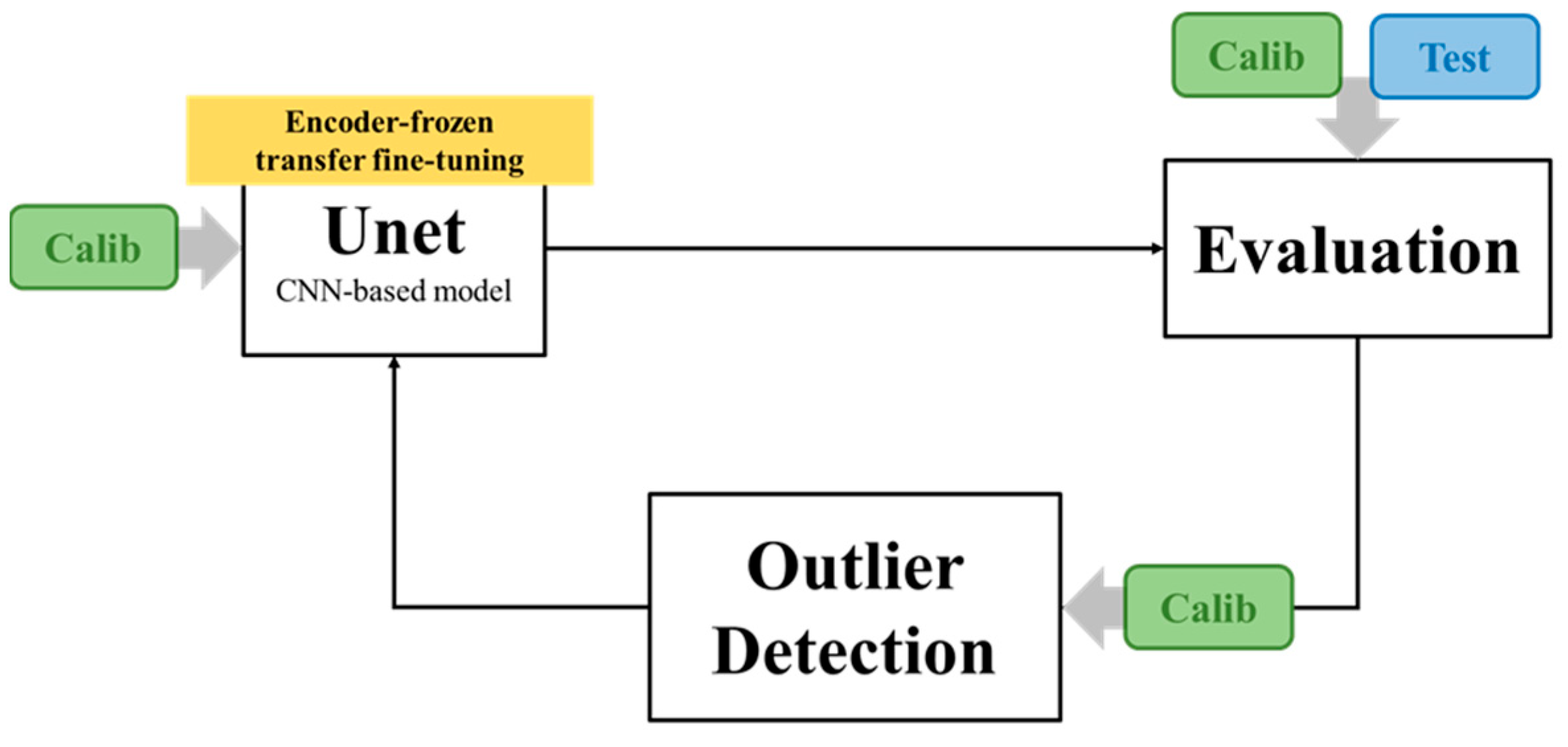
1.5. Calibration Flow and Transfer Learning

While CQR equips the model with calibrated and spatially adaptive prediction intervals, the further enhancement of predictive robustness requires more than a single-pass calibration. In the approach of the final step, we extend CQR with a structured calibration flow that continuously refines the model through outlier detection and spatial-aware reweighting on a fixed, limited calibration set.

This final step incorporates a low-cost yet effective transfer learning strategy, in which only the decoder and output layers of the baseline U-Net architecture are fine-tuned, while the encoder remains frozen to preserve generalized low-level features. Freezing the encoder during uncertainty-aware fine-tuning is a well-recognized approach for preserving foundational representation quality while adapting the task-specific outputs to more challenging spatial structures and boundary cases [17,33,42]. To guide this fine-tuning process, a pixel-level outlier-weighted map is computed based on conformal errors, with higher weights being assigned to spatial regions where the predicted intervals fail to capture the ground truth. These weights affect the per-pixel loss contribution during fine-tuning, allowing the model to focus its corrective updates on structurally uncertain or miscalibrated regions. Crucially, the entire calibration dataset—despite its small size—is reused in its entirety to make optimal use of valuable data to reinforce both local sensitivity and global consistency. Spatial outlier correction with reweighted fine-tuning in this valuable subset enables targeted correction without risking overfitting [43].

Recent studies have emphasized the value of such targeted fine-tuning routines, demonstrating improvements in predictive sharpness, uncertainty awareness, and generalization robustness even under constrained data settings. Alternative strategies, such as those proposed by Krishnan and Tickoo (2020), define differentiable calibration-aware loss functions that directly optimize confidence reliability rather than only predictive accuracy, paving the way toward robust and interpretable uncertainty-aware modeling frameworks [44].

1.6. Contribution and Scope of This Work

This study presents a closed-loop adaptive framework for progressive enhancement and the correction of layout-to-SEM image reconstruction, where model predictions are continuously improved using calibrated prediction intervals and pixel-level outlier detection. The approach presented first generates UQ results with formal statistical guarantees. An outlier map is then constructed from these results to identify and flag spatial regions with associated prediction risk. Finally, targeted model refinement is applied to improve reconstruction accuracy, particularly in these high-error regions, ensuring more reliable performance across the entire layout space. Such a closed-loop feedback process also enables a data-efficient and scalable approach for defect-aware model enhancement. This, in turn, facilitates robust layout-to-SEM prediction in practical NIL applications.

As a methodological contribution, this study introduces our integrated framework for uncertainty-aware pattern learning with tailor-made specific features to fit the semiconductor manufacturing in particular. The proposed pipeline combines the following:

(1)

A U-Net-based CNN model for hierarchical spatial feature learning;

(2)

CQR for interval-based predictions with statistical coverage guarantees;

(3)

Pixel-level outlier detection for localized uncertainty awareness;

(4)

An outlier-weighted fine-tuning strategy for enhancing adaptability to spatial variability.

Together, these steps constitute a unified and extensible platform supporting both predictive performance and uncertainty calibration. While the context has been explicitly illustrated here for NIL processes in particular, our framework is designed with a modular structure and pixel-level generality. This design choice renders the approach applicable to a wide variety of layout-driven semiconductor processes in general. It offers the potential for implementation across multiple stages of the manufacturing flow, including patterning, inspection, and defect-aware optimization as a whole.

2. Materials and Methods

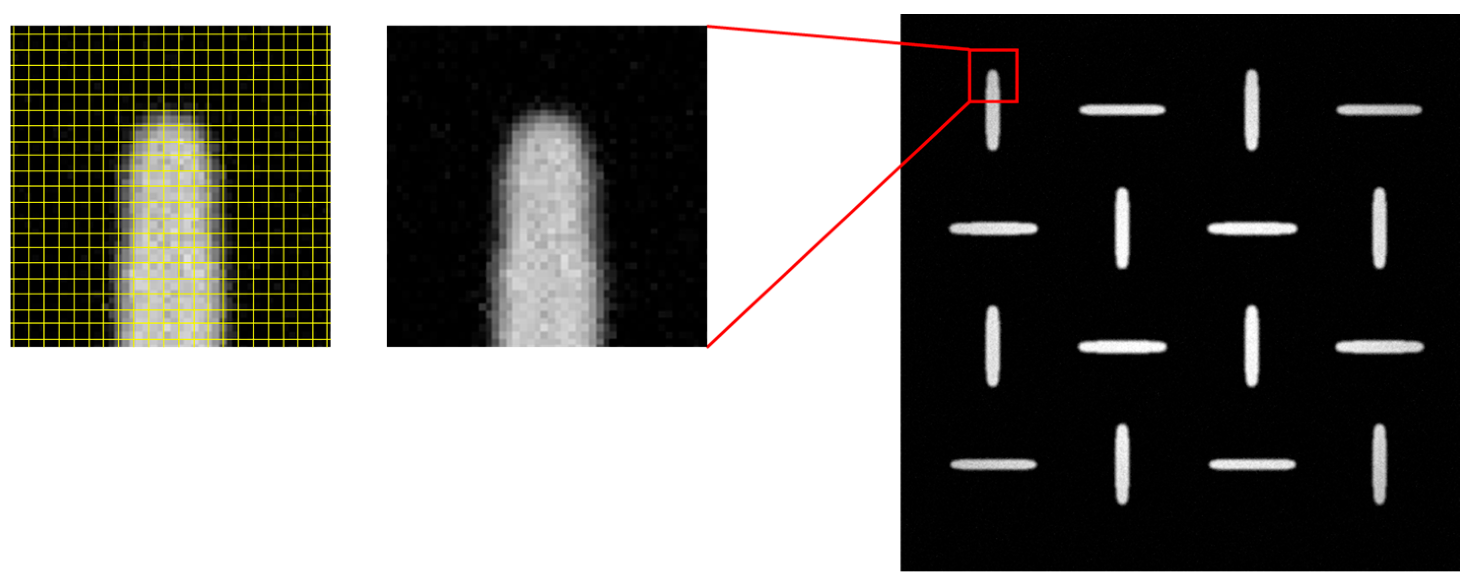
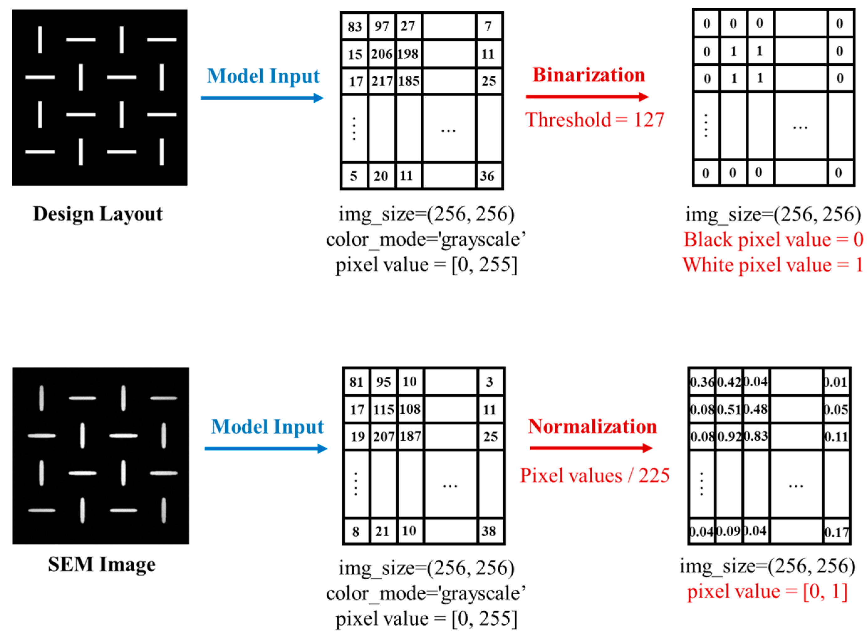
2.1. Dataset Preparation

To clearly analyze the actual NIL manufacturing process and apply custom optimization for this technology, we have developed a simulation framework based on physical principles rather than relying solely on data-driven heuristics. This framework incorporates key physical mechanisms across three integrated stages: electron beam lithography (EBL), reactive ion etching (RIE), and nanoimprint lithography (NIL).

In the EBL stage, the exposure distribution was simulated using a custom Python-based framework that implements a Gaussian dose blur with a full width at half maximum (FWHM) of 10–15 nm, along with proximity effect correction. These values reflect beam spreading observed in high-resolution systems and fast deflection regimes, spin-coated to a thickness of 180–200 nm, which balances resolution and etch durability [45,46,47,48]. During the RIE stage, the pattern transfer process was modeled using a custom Python-based level set simulation with angular dependence, tailored to SF₆/O₂ plasma conditions. The setup incorporates a chamber pressure of 10 mTorr, RF power of 100 W, and a vertical etch rate around 50 nm/min. To reflect directional etching and profile shaping, an anisotropy factor of 0.85 is included, following literature guidance on plasma profile evolution [49,50,51,52]. In the NIL stage, the resist is treated as a viscoelastic material following the Oldroyd-B model, with a zero-shear viscosity of approximately 5000 Pa·s and relaxation time of 0.02 s, representative of UV-curable imprint materials commonly used in NIL applications [53,54,55].

To visualize the resulting structures, we convert simulated height maps into grayscale SEM-like images using a surface-rendering procedure inspired by Seeger and Haussecker (2005) [56]. This includes the following:

(1)

Contrast shading according to local height gradients to mimic secondary electron emission variation over surface slope [57];

(2)

Gaussian blur to simulate depth-of-field softness typical of SEM systems [58];

(3)

Additive Gaussian noise to account for beam fluctuation and detector imperfection [59].

A representative zoom-in is shown in Figure 1, highlighting surface detail, shape continuity, and grayscale falloff—features that collectively reproduce the appearance characteristics seen in actual SEM micrographs. By integrating these stages—EBL exposure modeling, RIE pattern transfer, and NIL deformation simulation—the framework captures critical spatial dynamics across fabrication steps. This simulation engine serves not only to generate training images but also to preserve physical realism at the nanoscale. A dedicated manuscript detailing this physics-based simulation framework is currently in preparation. Both studies were developed in parallel but submitted separately due to differing journal scopes and submission timelines.

Our data management strategy involves the division of the design layouts and the corresponding SEM target images into four independent subsets, training, validation, calibration, and test, based on a 60:18:12:10 split. All subsets are statistically dependent, but distinctive from spatial and structural variations of the design layouts, though they originate from the same process domain. The distinction allows for fair model evaluation and generalization, which is crucial for UQ and robust performance validation in downstream tasks such as OPC verification and defect-aware process learning.

To enhance pattern diversity and promote more comprehensive spatial variation learning, we applied deterministic data augmentation through fixed-angle rotations [18]. In particular, each original image was rotated by 90°, 180°, and 270°, resulting in three additional geometrically transformed variants for every input. This effectively expanded the dataset size by a factor of four. These rotational transformations also hold significant physical relevance in the context of NIL, as the pattern symmetry in layout designs is typically an exhibition of rotational invariance, making this form of augmentation particularly suitable for mask-based pattern prediction tasks.

All images were preprocessed to match a fixed resolution of 256 × 256 pixels. This resolution was selected as a balance between geometric fidelity and computational efficiency. In our dataset, each layout image usually has one primary pattern unit, named contour, which corresponds to a local structural feature. The resolution of 256 × 256 pixels provides sufficient detail to preserve the shape and boundary information of each contour. If fewer pixels were used (i.e., lower resolution), each pixel would cover a larger physical area. This would increase the risk of ambiguity along the boundary between the contour and the background, and could cause errors in local feature interpretation as well as reduce the overall prediction accuracy of the model. On the other hand, using a higher resolution would dramatically increase training and inference computational cost without proportionate gains in learning performance. Therefore, 256 × 256 serves as a practical trade-off that maintains essential topological information without excessive training complexity.

Design mask layout patterns were binarized with a fixed intensity threshold of 127 for maintaining topological consistency, whereas SEM images were normalized into the [0, 1] range by dividing pixel values by 255.0 for stable convergence during CNN training. These preprocessing steps, shown in Figure 2, not only ensure physical interpretability, numerical stability, and generalization, but also enhance model training effectiveness. This is particularly critical under conditions of limited data availability and measurement uncertainty, which are common in high-resolution semiconductor manufacturing process modeling scenarios.

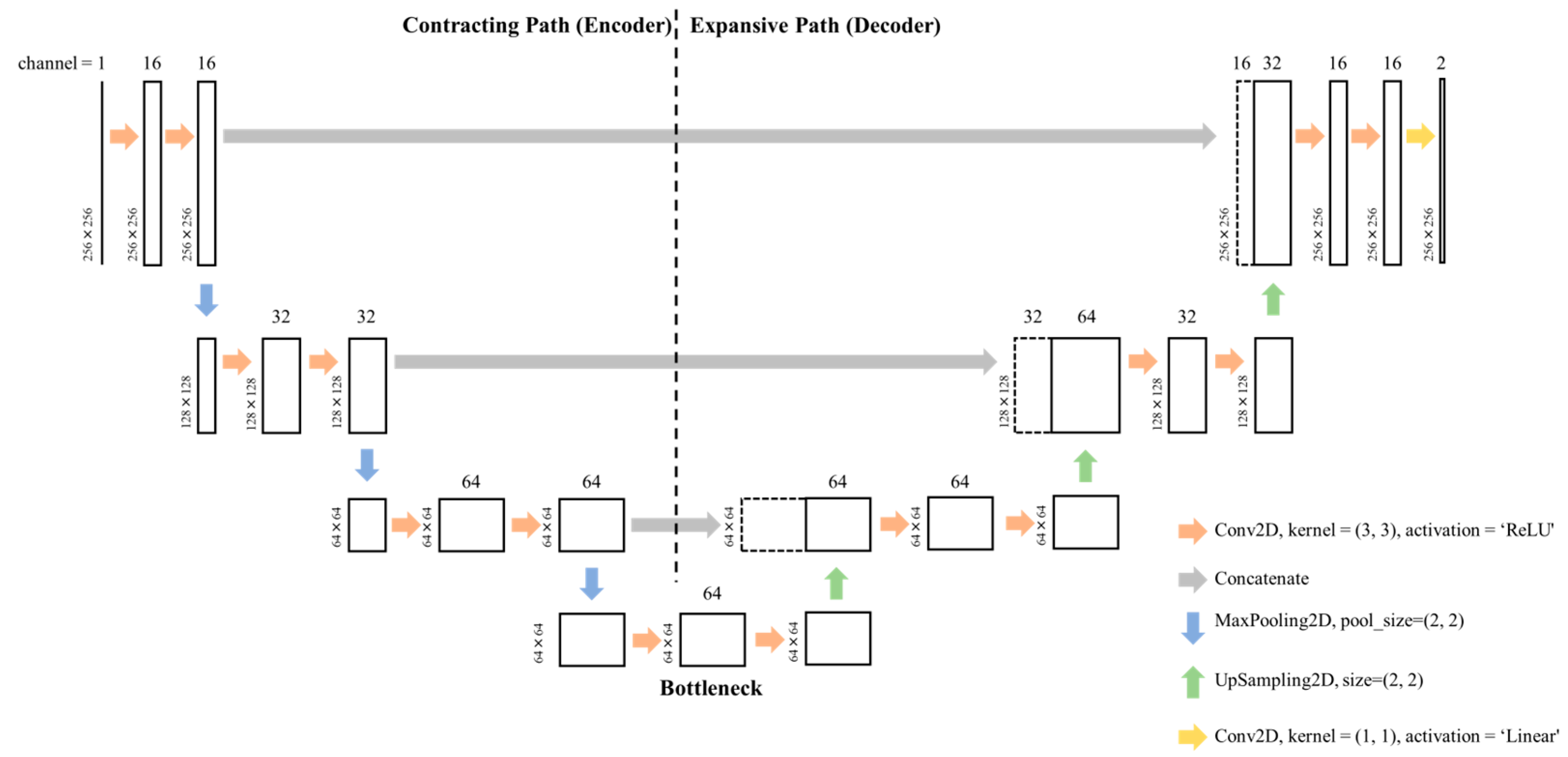
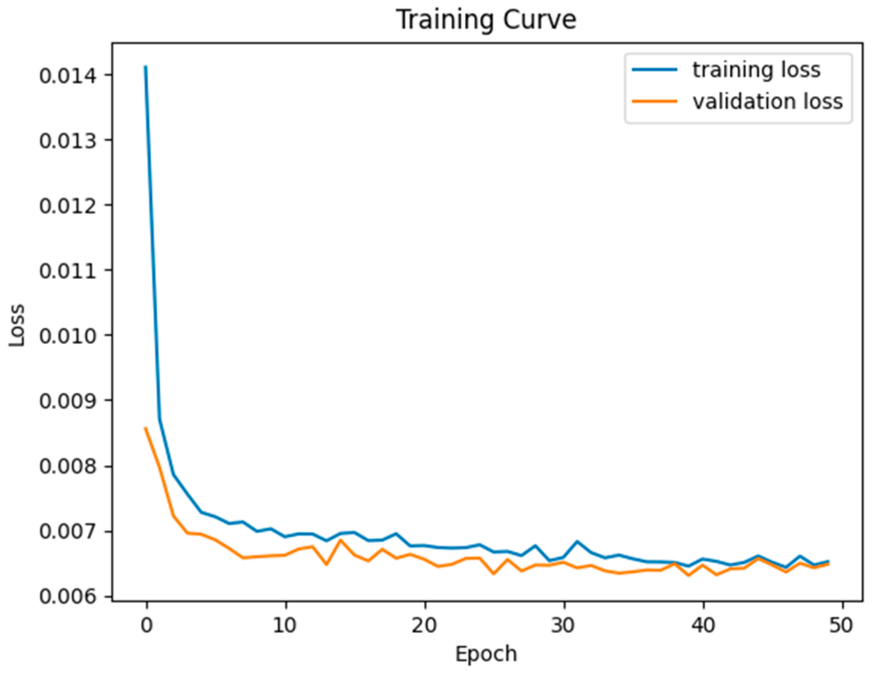
2.2. CNN-Based Model and Training

For performing pixel-by-pixel prediction of grayscale SEM images from binary mask layouts, we employed a U-Net-based CNN architecture. The U-Net model, originally developed by Ronneberger et al. for biomedical image segmentation [20], is a convolutional autoencoder designed for encoding both global context and subtle spatial details through a symmetric encoder–decoder structure with skip connections. The model is named “U-Net” due to the distinctive U-shaped architecture formed by its contracting and expansive paths, which mirror each other across a bottleneck layer. In our study, we used a shallow variant of U-Net to fit the limited training dataset and prevent overfitting, without losing the essential properties of spatial localization and low-level feature retention.

As shown in Figure 3, the proposed architecture consists of three main components: a contracting path (encoder), a bottleneck, and an expansive path (decoder). The contracting path is responsible for downsampling the input along with learning hierarchical features. It contains two convolutional blocks, each comprising two consecutive 3 × 3 convolutional layers with ReLU activation and zero-padding, followed by a 2 × 2 max-pooling operation that halves spatial resolution. The number of filters rises from 16 to 32 as we go deeper into the network. This design allows the encoder to progressively capture sophisticated fine-grained features while compressing the spatial dimensions from 256 × 256 to 64 × 64.

The encoder is then followed by a bottleneck module, consisting of two 3 × 3 convolutional layers with 64 filters and ReLU activation. The bottleneck in our shallow model, which serves as the most compressed representation of the input [60], has a spatial resolution of 64 × 64. It still preserves essential spatial information, which, in turn, helps achieve a balance between semantic abstraction and localization capacity. Semantic abstraction refers to the capacity of the model to understand what is in the image, such as edges, textures, or structural regions. Localization capacity, on the other hand, means having the capacity to retain the spatial context of each feature with respect to the original spatial layout. In typical deep U-Net models, having deeper bottlenecks can enhance semantic encoding but at the cost of losing spatial details. In contrast, our shallow U-Net maintains a relatively large feature map (64 × 64) at the bottleneck stage. Here, in turn, it helps to preserve fine-grained spatial resolution while it still benefits from hierarchical representation. This structure ensures that the model can simultaneously capture significant features and preserve pixel-level accuracy.

The expansive path reconstructs the feature maps back to the original input resolution. It consists of two upsampling steps of 2 × 2 nearest-neighbor upsampling, followed by concatenation with the corresponding feature maps from the encoder (skip connections), and two 3 × 3 convolutional layers with ReLU activation. These skip connections, through which low-level spatial information directly passes from the encoder to the decoder, preserve fine-grained boundary details that are typically lost during downsampling. The number of filters keeps decreasing from 64 to 32, and then 16, in the output layers. Finally, one 1 × 1 convolutional layer with two output channels is used to provide two continuous-valued output maps corresponding to the predicted lower and upper quantiles of the SEM grayscale intensity. The model takes as input grayscale images of size (256, 256, 1) and produces a final output tensor of size (256, 256, 2), thereby allowing simultaneous quantile prediction for each pixel.

Given the relatively small size of the dataset (24 training images with 4× augmentation), this shallow version of the U-Net is a good trade-off between model expressiveness and generalization. Decreasing the depth reduces the overfitting risk without sacrificing the structural advantages of the U-Net design. The model is trained using a conformalized quantile regression custom loss function described in the following section.

The GPU hardware specifications and training configurations are summarized in Appendix A.1, while the architectural and optimization hyperparameters are listed in Appendix A.2.

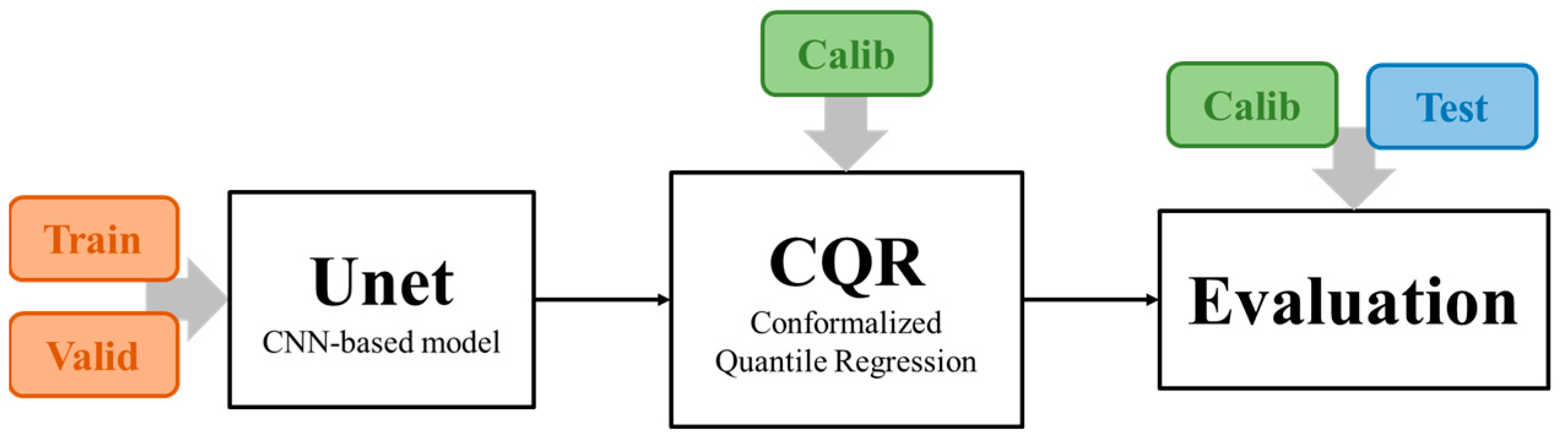
2.3. Conformalized Quantile Regression (CQR)

In order to implement the UQ of our shallow U-Net model, we apply conformalized quantile regression (CQR), which teaches the ability to predict lower and upper quantile bounds for each pixel’s grayscale SEM value simultaneously. The loss function relevant to CQR is defined as a sum of asymmetric pinball losses (${\mathcal{L}}_{q_{low}}, {\mathcal{L}}_{q_{high}}$) for two different quantiles:

$${\mathcal{L}}_q\left(y,\widehat{y}\right)={\displaystyle \frac{1}{HW}}{\sum }_{i,j}\left[max\left(q\left(y_{ij}-{\widehat{y}}_{ij}\right),\left(1-q\right)\left(y_{ij}-{\widehat{y}}_{ij}\right)\right)\right]$$

(1)

$${\mathcal{L}}_{CQR}={\mathcal{L}}_{q_{low}}\left(y,{\widehat{y}}^{low}\right)+{\mathcal{L}}_{q_{high}}\left(y,{\widehat{y}}^{high}\right)$$

(2)

Here, H × W = 256 × 256 corresponds to the spatial resolution of a single grayscale SEM image, i.e., the total number of pixels per image. $y_{ij}\in \left[\mathrm{0,1}\right]$is the normalized ground truth SEM value. ${\widehat{y}}^{low}$, ${\widehat{y}}^{high}$ represent the predicted quantiles for a specified confidence level. In our case, we set $q_{low}=0.05$ and $q_{high}=0.95$, corresponding to a 90% prediction interval.

Following the first training phase, a conformal calibration procedure is performed on a held-out calibration set to find the necessary quantile threshold to achieve the target coverage level and, hence, ensure reliable uncertainty quantification. For each pixel in the calibration data, the conformal error $e_{ij}$ is computed as follows:

$$e_{ij}= max \left({\widehat{y}}_{ij}^{high}-y_{ij},y_{ij}- {\widehat{y}}_{ij}^{low}\right)$$

(3)

The calibration constant $q^{*}$ is then determined as the empirical of the set of errors:

$$q^{*}= {Quantile}_{1-\alpha }\left({\left\{e_{ij}\right\}}^{H\times W}\right)$$

(4)

Under the exchangeability assumption, this condition guarantees that the prediction interval is statistically valid across the calibration distribution:

$$P_{x\sim \mathcal{D}} \left[y_{ij}\left(x\right)\in \left[{\widehat{y}}_{ij}^{low}\left(x\right)-q^{\mathrm{*}},{\widehat{y}}_{ij}^{high}\left(x\right)+q^{\mathrm{*}}\right]\right]\ge 1-\alpha$$

(5)

Here, $\alpha = 0.1$ denotes the rate of miscoverage. For a new input $x$ sampled from the same distribution $\mathcal{D}$, the ground truth $y_{ij}\left(x\right)$ must lie in the calibrated interval $\left[{\widehat{y}}_{ij}^{low}\left(x\right) -{ q}^{*},{\widehat{y}}_{ij}^{high}\left(x\right)+ q^{*} \right]$ with probability of at least $1-\alpha$. Exchangeability makes sure that the calibration set, as a subset drawn from the same distribution, enables the model to generalize its robust prediction intervals to unseen but similar distributed patterns.

2.4. Outlier-Weighted Calibration and Transfer Learning

To further improve the reliability and spatial accuracy of the layout-to-SEM image reconstruction task under the constraints of process-induced uncertainty—including aleatoric variability from lithographic or SEM noise and epistemic uncertainty due to limited data or model underfitting—we employ a conformal calibration strategy with a transfer learning pipeline based on Section 2.2 and Section 2.3. This phase aims to enhance both the calibration quality and spatial accuracy of predictions in lithographically sensitive regions. Emphasis is placed on scenarios with sparse data and on structurally complex regions, including feature edges and imprint-induced residual defects. This is especially crucial in NIL process windows involving low residual layer thickness or incomplete release, where SEM intensity variations point out the potential defect onset.

The proposed calibration flow consists of three main steps: (1) base quantile model calibration, (2) outlier-enhanced pixel-by-pixel weighting strategy, and (3) encoder-frozen transfer fine-tuning.

(1) Base quantile model calibration. Following the base quantile model calibration described in Section 2.3, we adopted the empirically estimated calibration constant$q^{*}$ to construct valid pixel-level prediction intervals $\left[{\widehat{y}}_{ij}^{low}\left(x\right)-q^{*},{\widehat{y}}_{ij}^{high}\left(x\right)+q^{*} \right]$ with guaranteed marginal coverage of at least $1-\alpha$. This post-CQR prediction intervals provide the foundation for the subsequent fine-tuning strategy.

(2) Outlier-enhanced pixel-by-pixel weighting strategy. To emphasize structurally critical regions during fine-tuning, we introduce an outlier-enhanced pixel-by-pixel weighting strategy through conformal prediction analysis. This strategy assigns greater weight to regions of increased uncertainty, so the model pays more attention to spatial locations with higher predictive deviation. For each pixel in the calibration dataset, we calculated the conformal error $e_{ij}$and calibration constant $q^{*}$ earlier in Equations (3) and (4). Here, $q^{*}$ presents as the global outlier threshold. Pixels for which the error exceeds $q^{*}$ are considered outliers and are assigned higher weights. The pixel-by-pixel weight map is then defined as follows:

$$w_{ij}= \left\{\begin{array}{c}\gamma if e_{ij}>q^{*}\\ 1.0 otherwise\end{array}\right.$$

(6)

Here, $\gamma >1$is a scalar denoting the level of reweighting, set to 1.3 in our experiments. The pixel-by-pixel weight maps were directly concatenated with the ground truth images to form a 2-channel training target tensor, as shown in Equation (7), of shape (256, 256, 2), where the first channel represents the normalized ground truth and the second channel holds the corresponding pixel weights.

$${\tilde{y}}_{ij}=\left[y_{ij}, w_{ij}\right]$$

(7)

By guiding the loss function to focus on pixels with greater uncertainty violations, this strategy enables the model to adaptively correct outlier regions—particularly those near feature edges or NIL-induced residual hotspots—without compromising performance in already well-calibrated regions. The resulting weight maps are seamlessly integrated into the CQR loss during the transfer fine-tuning stage, allowing targeted recalibration of uncertain regions using existing labels only, thereby improving reliability under limited-data conditions.

(3) Encoder-frozen transfer fine-tuning. To mitigate catastrophic forgetting from the initial U-Net training while enabling targeted local adaptation during fine-tuning, we adopted a transfer learning strategy in which the encoder of our baseline U-Net model was frozen, and only the decoder and output layers were fine-tuned. This ensures that the low-level feature extraction of the baseline model remains intact while allowing targeted improvement in regions previously prone to high prediction errors or structural uncertainty outliers. Let the original model parameters be denoted as $\theta =\left\{{\theta }_e, {\theta }_d\right\}$, where ${\theta }_e$and ${\theta }_d$correspond to the encoder and decoder parameters, respectively. During fine-tuning, we imposed the following constraint:

$${\theta }_e^{transfer}={\theta }_e^{base}, with {\displaystyle \frac{\partial \mathcal{L}}{\partial {\theta }_e^{transfer}}}= 0$$

(8)

This enforces that encoder parameters remain unchanged, that is, to ensure there are no gradient updates applied to the encoder parameters. The transfer fine-tuning is performed on the calibration set, where ${\tilde{y}}_{ij}$ in Equation (7) represents the reweighted label constructed by appending the pixel-by-pixel weight map $w_{ij}$, based on our outlier-enhanced weighting strategy described in Equation (6). We retained the fine-grained pixel-by-pixel weighting directly within the fine-tuning objective function by embedding the weight map $w_{ij}$ into the conformal quantile regression loss. The resulting fine-tuning function objective is defined as follows:

$${\mathcal{L}}_q^{weighted}\left(y,\widehat{y}\right)={\displaystyle \frac{1}{HW}}{\sum }_{i,j}{w}_{ij}\left[max\left(q\left(y_{ij}-{\widehat{y}}_{ij}\right),\left(1-q\right)\left(y_{ij}-{\widehat{y}}_{ij}\right)\right)\right]$$

(9)

This formulation enables pixel-by-pixel error correction in spatially localized outlier regions, such as nanoscale hotspots or residual imprinting defects, while maintaining overall stability in structurally consistent areas. It further allows the decoder to recalibrate the predictive uncertainty while preserving the high-level semantic information of the encoder. After training, the fine-tuned model is evaluated alongside the baseline model using a unified evaluation framework. Specifically, both models are compared under a consistent metric, where pixel-by-pixel outliers are identified based on the same calibrated threshold $q^{*}$, and prediction validity is measured via coverage rate. These metrics provide a fair basis to quantify the improvement of the model in uncertainty calibration and spatial accuracy.

2.5. Evaluation Metrics

After concluding the two-stage calibration procedure of Section 2.3 and Section 2.4 for both the baseline U-Net model and its transfer fine-tuned model, they are evaluated under a unified, application-specific framework designed specifically to the needs of OPC. The evaluation is based on two primary performance metrics, Mean Absolute Error (MAE) and Prediction Interval Coverage, which collectively determine the accuracy and reliability of the predicted SEM intensity profiles.

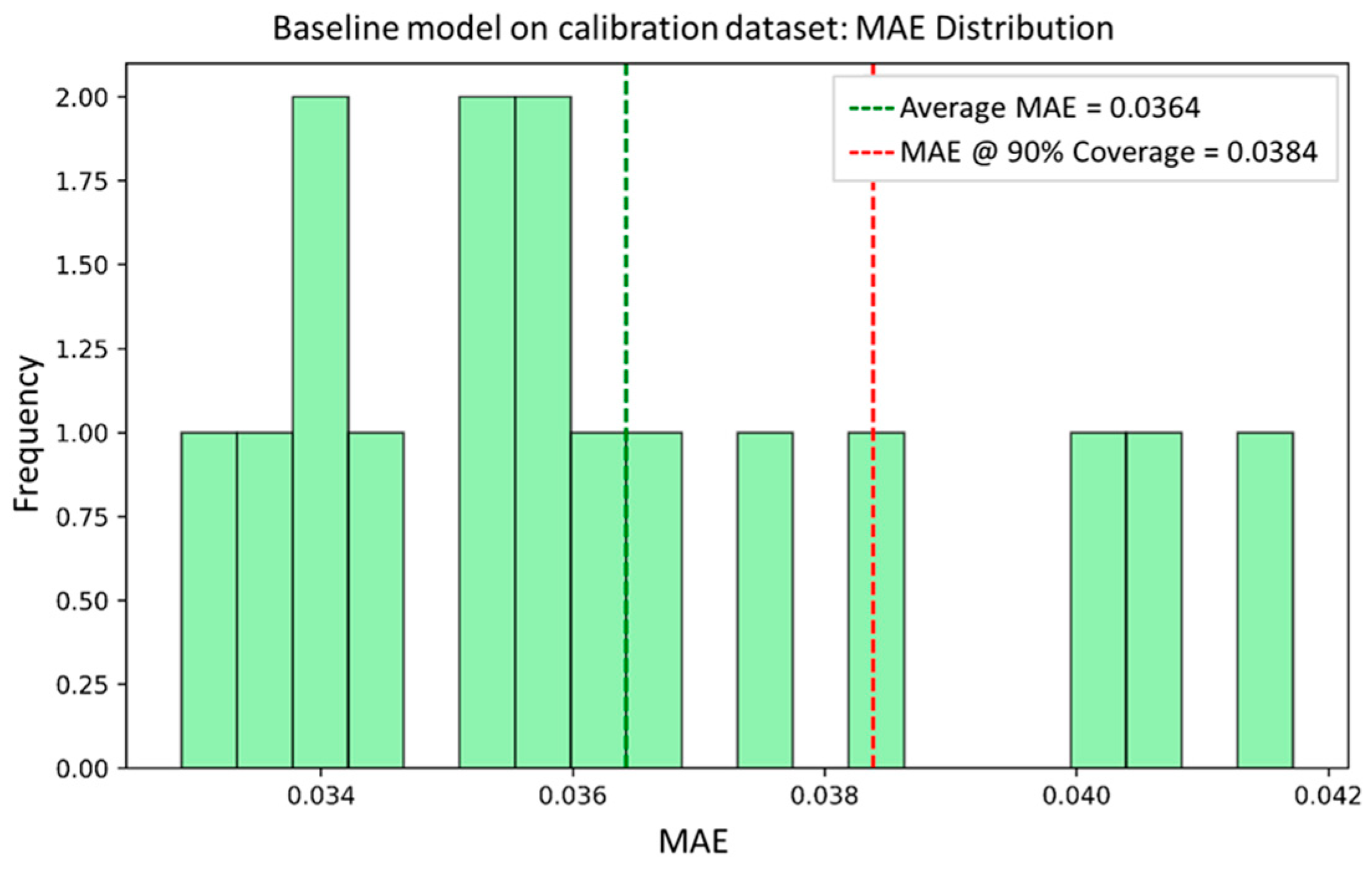
2.5.1. Mean Absolute Error (MAE)

To evaluate pixel-level accuracy, we introduce the MAE between the midpoint of the predicted quantile bounds and the corresponding ground truth pixel value. It serves as a critical measure of local feature accuracy, particularly reflecting how well fine-scale shape variations and edge positions are preserved. The formula is as follows:

$$MAE ={\displaystyle \frac{1}{HW}}{\sum }_{i,j}\left|{\displaystyle \frac{1}{2}}\left({\widehat{y}}_{ij}^{low}\left(x\right)+{\widehat{y}}_{ij}^{high}\left(x\right)\right)-y_{ij}\right|$$

(10)

In our setting, H × W = 256 × 256, indicating that each SEM image has 256 × 256 pixels. The quantile midpoint used here offers a stable estimate of the predicted surface profile, balancing the upper and lower bounds to provide a reliable pixel-wise estimate. In OPC applications, low MAEs are essential to meet in-fab tolerance requirements, with sub-pixel deviations often acceptable depending on design rules.

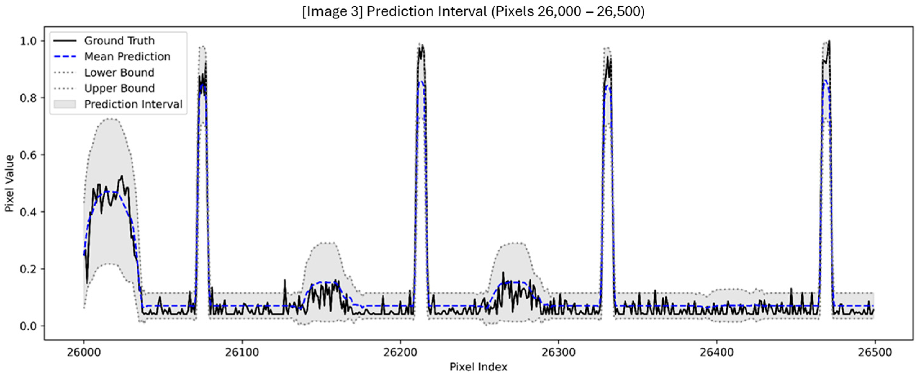
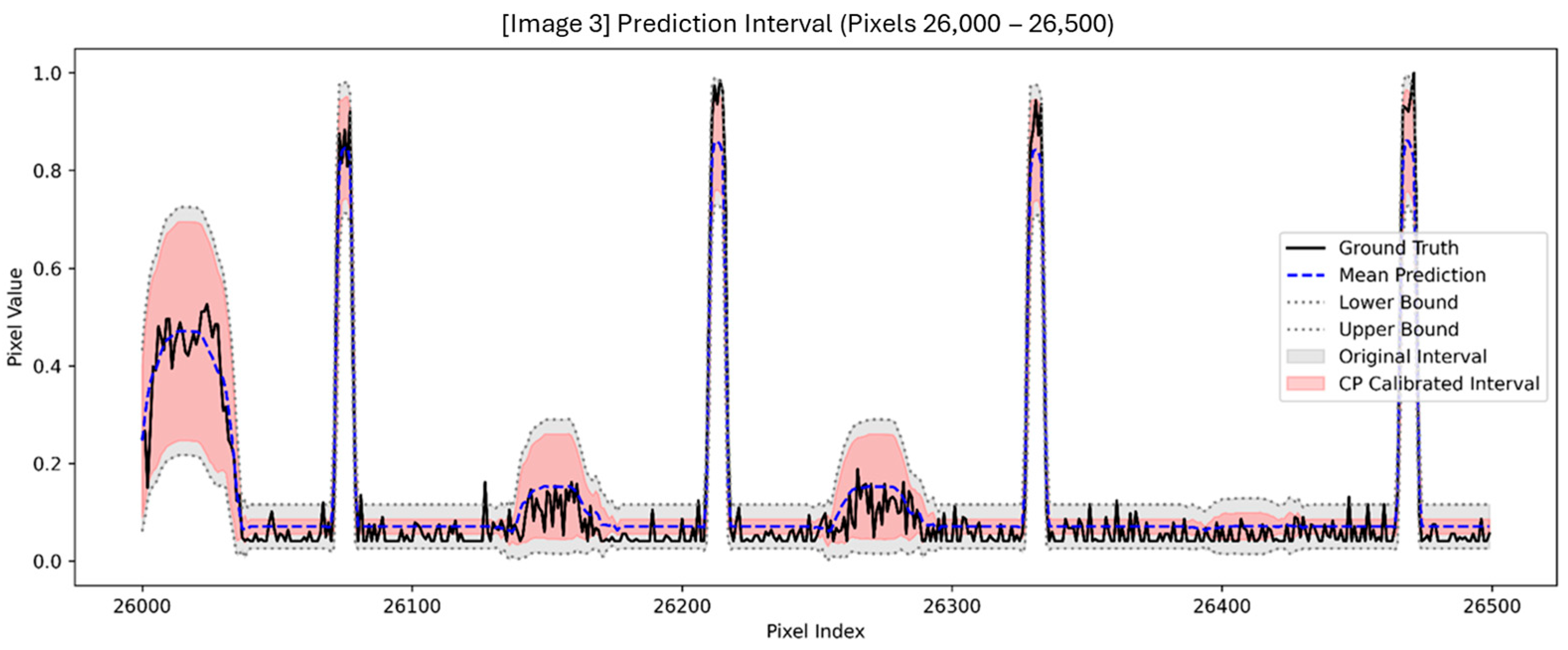
2.5.2. Prediction Interval Coverage

To quantify the reliability of uncertainty, we calculate the coverage rate, or the proportion of ground truth values that fall within the conformal prediction interval:

$$Coverage ={\displaystyle \frac{1}{HW}}{\sum }_{i,j}1\left\{y_{ij}\in \left[{\widehat{y}}_{ij}^{low}-q^{\mathrm{*}},{\widehat{y}}_{ij}^{high}+q^{\mathrm{*}}\right]\right\}$$

(11)

For a consistent evaluation process, the same calibration constant $q^{*}$ is used for both baseline and transfer fine-tuned models. This strategy supports a more meaningful and informative model comparison by making an explicit test of whether transfer fine-tuning can reduce the outlier regions identified in the baseline model. This approach aligns with our goal to evaluate the performance of transfer fine-tuning in correcting pixel-by-pixel uncertainty-aware prediction errors.

3. Results

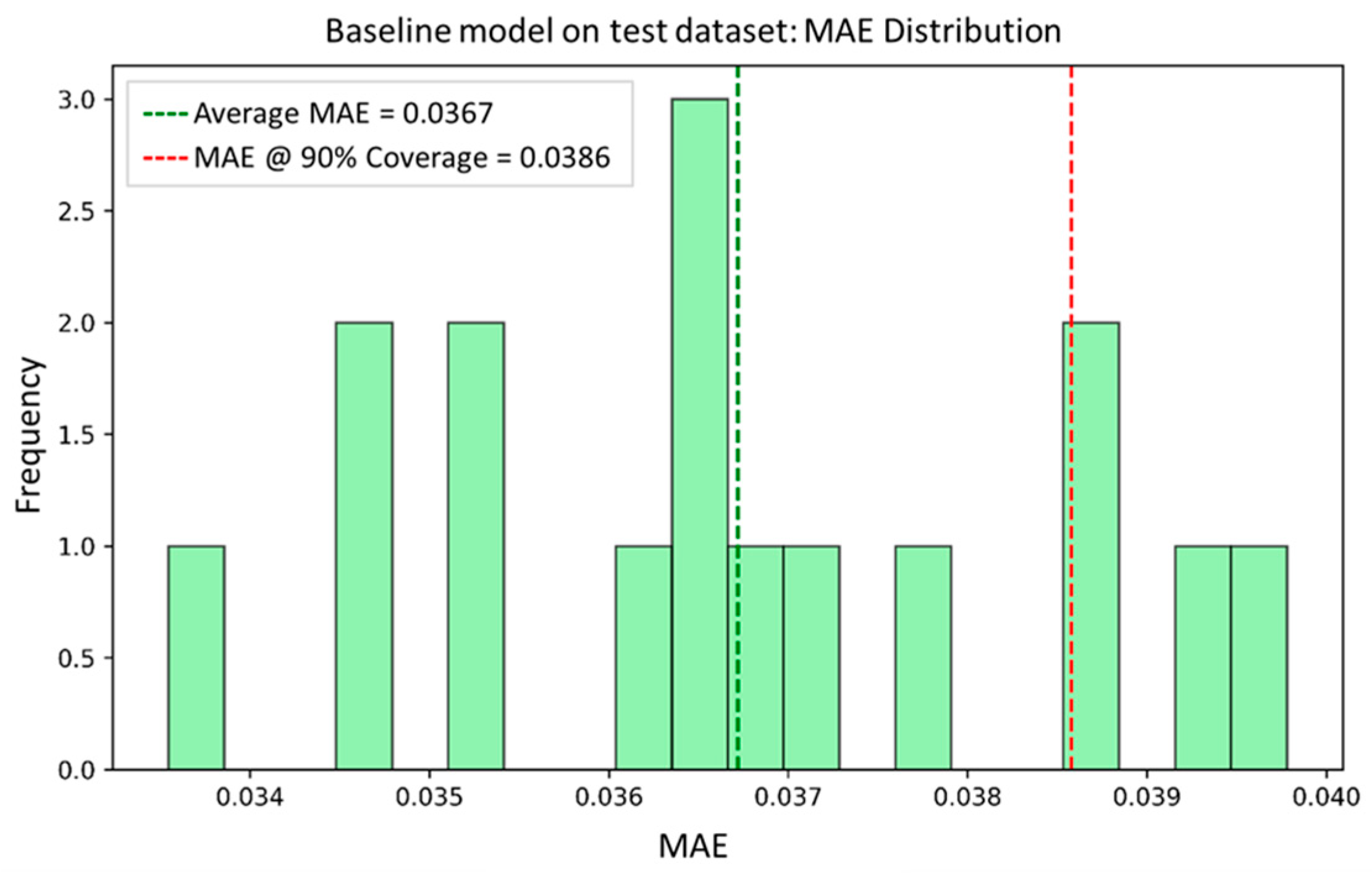
3.1. Baseline Evaluation

The baseline pipeline, illustrated in Figure 4, involves training a U-Net together with CQR to estimate the pixel-by-pixel prediction intervals for SEM image reconstruction. The network outputs both lower and upper bounds for every input layout, enabling spatially resolved UQ. The mean prediction for evaluation is provided by the average of the lower and upper bounds and is the point estimate chosen to represent the target image. Representative patterns and corresponding model predictions are illustrated in Figure 5. To further observe the model convergence and generalization performance, the loss curves for both the training and validation phases are provided in Figure 6.

The inclusion of noise in the SEM images generated from previous physical modeling is to emulate realistic imaging conditions. These SEM images, produced through physics-based simulation, serve as training targets for the baseline U-Net model. Since real SEM images inherently contain background noise, charging effects, and structural distortions, we simulate such imperfections by incorporating controlled noise during training. This allows the model to be more tolerant of these realistic artifacts. This step not only enables an evaluation of the model’s capacity to generalize from synthetic to real SEM domains but also mitigates the risk of overfitting to unrealistically perfect synthetic data, thereby enhancing the robustness of the learned representations.

The U-Net model, guided by CQR through the prediction of lower and upper quantile bounds for each pixel, naturally highlights features with pixel values around 1.0 (contours and patterns) while reducing the effect of background noise around 0.0. This focused attention allows the accurate reconstruction of essential structural features by increasing the contrast between patterned and non-patterned regions, resulting in sharper and more clearly defined boundaries. Figure 7 illustrates a pixel-by-pixel comparison of the ground truth and the model prediction intervals over a selected region (Pixels 26,000–26,500). The ground truth curve (black) shows high-frequency noise and fluctuation in low-intensity regions, as is commonly observed in SEM imaging due to charging effects or stochastic process variation. Conversely, the mean prediction (blue dashed line) exhibits significant denoising capability, successfully reconstructing the signal profile while effectively filtering out background noise. Furthermore, the prediction intervals (gray band between lower and upper bounds) remain a consistently narrow and stable range, especially in flat regions, indicating a high level of model confidence and limited uncertainty. This stability provides additional confirmation that the model effectively prevents local overfitting in small background segments and demonstrates commendable generalization performance in both high-contrast and low-intensity regions.

A comparison of ground truth values and predicted quantile intervals, as shown in Figure 8, reveals that uncertainty is small in background regions and highest along edges, where pattern fidelity is most sensitive. This observation is consistent with the physical behavior in NIL processes, where post-imprint template release often results in local resist deformation near sidewalls due to surface tension or adhesion forces. These effects introduce geometric uncertainty in the reconstructed contours, as reflected in the increased prediction error at boundaries.

The pixel-by-pixel error distribution indicates an MAE of 0.0364, with errors concentrated at the edge of each patterned unit as shown in Figure 8. This regular and physically explainable uncertainty motivates the need for post-training calibration. By applying CQR calibration using a held-out dataset, the errors are sorted to determine a quantile threshold $q^{*}= 0.0617$, which regulates the prediction interval to cover 90% of the true pixel values. This calibrated bound, as shown in Figure 9, ensures the statistical validity of the model’s confidence intervals and forms the basis for further refinement in the subsequent calibration–transfer workflow.

After applying CQR to the prediction intervals of the baseline U-Net model, we obtain calibrated bounds that provide 90% pixel-by-pixel coverage with respect to a given error threshold. This calibration ensures that, with a high statistical confidence, the prediction intervals contain the true pixel values, which directly allows an estimate of bounded MAEs.

To visualize the distribution of MAEs within the dataset, histograms of the calibration and test datasets are shown in Figure 10 and Figure 11, respectively. The green dashed line in each figure indicates the average MAE, while the red dashed line represents the MAE at the 90th percentile of errors. In the calibration dataset, the average MAE is 0.0364 and the 90% coverage MAE is 0.0384. Consistent with the calibration results, the test dataset shows slightly higher values—0.0367 and 0.0386, respectively. These minor differences, confined to the fourth decimal place, are well within acceptable bounds and reflect the expected structural and spatial variability intentionally preserved between the subsets. Given the fact that the calibration and test datasets are sampled from distinct layout regions originating from the same process domain, such deviation supports the robustness and generalizability of the conformal calibration framework rather than indicates overfitting or model bias. This confirms that the model maintains consistent MAE behavior over different layout instances, which validates its utility for uncertainty-aware downstream applications such as OPC verification and lithographic process optimization.

Furthermore, this statistically consistent behavior enables the definition of outliers by thresholding the MAE beyond the 90% coverage bound. As we will demonstrate in the following outlier map analysis, the calibrated uncertainty region provides a meaningful reference to identifying regions where model predictions become less reliable, thereby supporting uncertainty-aware model diagnosis and confidence-aware pattern evaluation.

Figure 12 presents outlier maps for selected samples from the test dataset, where outliers are defined as pixels whose MAE exceeds the conformal threshold of 0.0384. In these plots, red pixels indicate regions where the prediction of the model deviates beyond the calibrated uncertainty intervals, while green pixels indicate areas that are still within the specified tolerance. In all four plots, there is an evident spatial pattern: most of the outliers are concentrated near the contour boundaries of the pattern features, especially along the elongated edges where the physical process variation and resist behavior are more pronounced. This aligns with expectations based on the physics of NIL, in which edge defects and residual deformation are more likely to introduce structural uncertainty.

The increased uncertainty and MAE near feature boundaries, as seen in Figure 8 and Figure 12, are consistent with the epistemic uncertainty arising from the limited structural generalization. In comparison, the narrow and stable intervals observed in background regions suggest that aleatoric noise is effectively captured by the model.

The large number of outliers in the test dataset indicates that, although the model is strong on average performance, there remain localized regions with a lower confidence and severe prediction error. This demonstrates the need for improvement beyond global conformal calibration. In particular, it motivates the development of an outlier-weighted calibration framework that can selectively adjust prediction outputs based on local reliability. It also promotes the use of transfer learning techniques to improve generalization on previously unseen pattern types. The results of these form the foundation for the next section, in which we present an outlier-weighted calibration and transfer learning method that aims to promote robustness and spatial generalizability in uncertainty estimation.

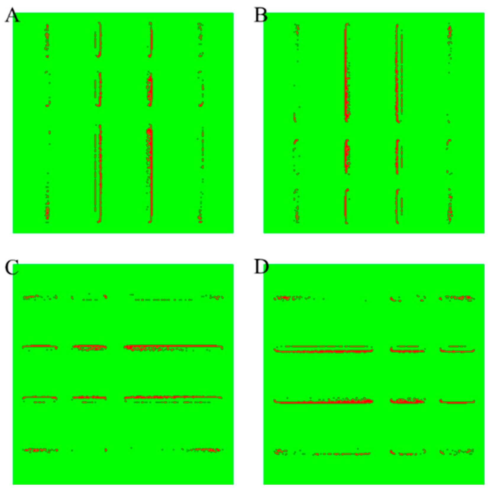
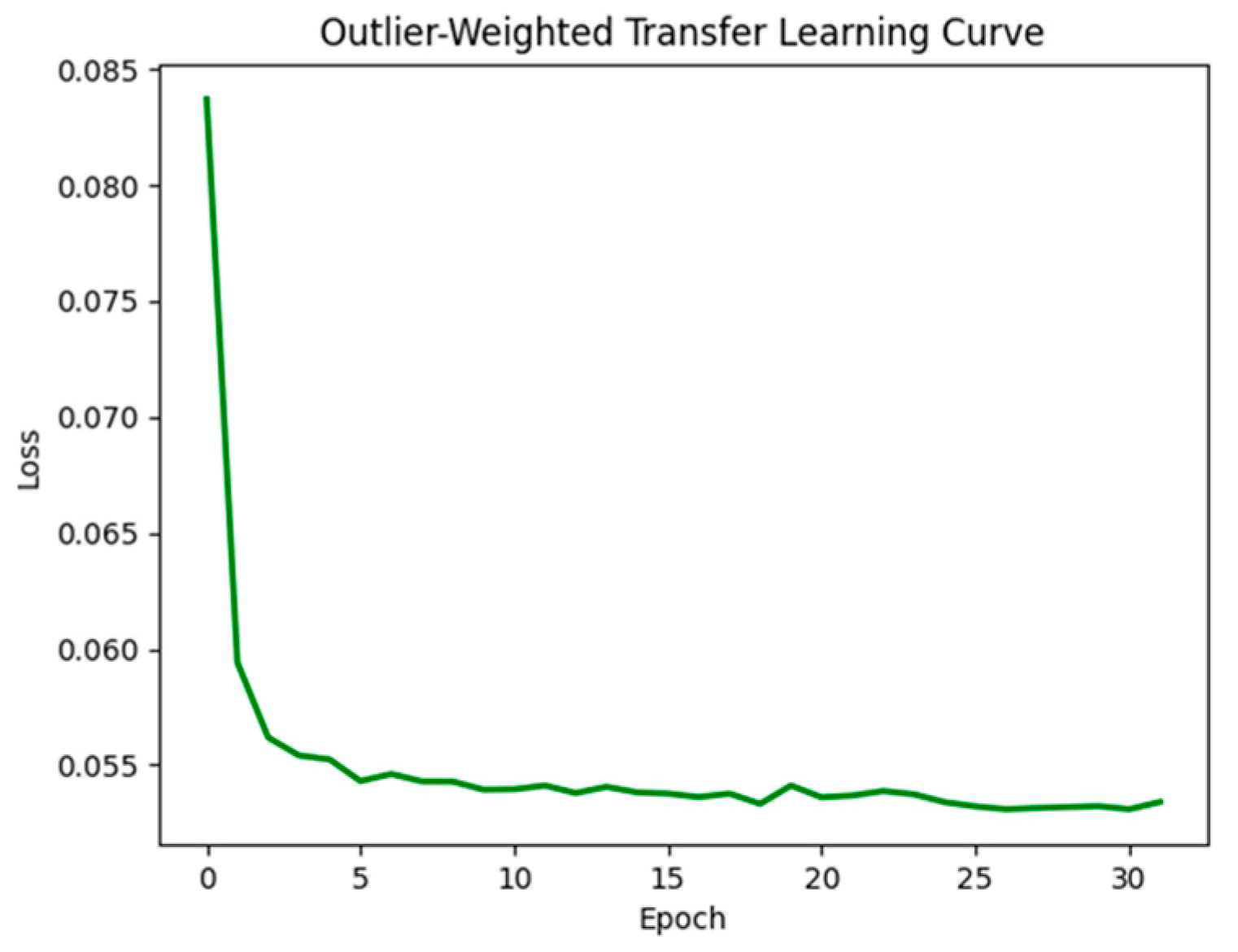
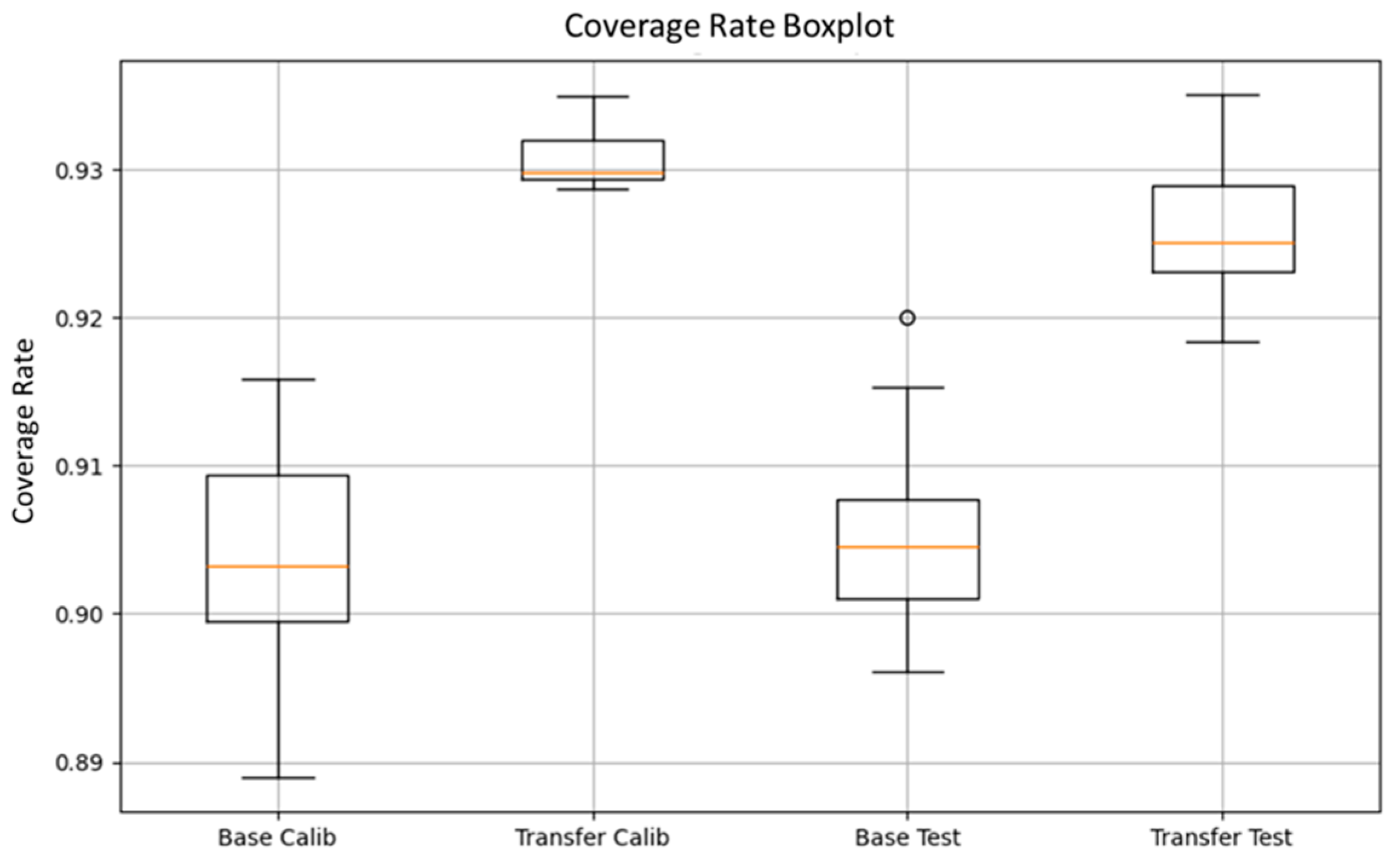
3.2. Outlier-Weighted Calibration and Transfer Learning Evaluation

As shown in Figure 13, the transfer learning pipeline starts by evaluating the baseline U-Net model through a held-out calibration dataset. The conformal errors derived from this evaluation are then utilized for outlier detection, where pixels fail to meet the pre-specified coverage. Based on the specific downstream target (e.g., the minimization of MAE, Line Edge Roughness (LER), or CD Uniformity (CDU)), practitioners can establish case-by-case specific thresholds for outlier detection. In our case, we apply the conformal 90% coverage criterion, treating deviations beyond this interval as meaningful indicators of outliers in the model. The identified outliers are then sent to the next phase: the outlier-enhanced pixel-by-pixel weighting strategy and encoder-frozen transfer fine-tuning, the pipeline that reweights the loss function at the pixel level, updates the decoder layers only to enhance local prediction accuracy, and then preserves global structural representation.

Figure 14 illustrates the training loss curve across 33 epochs during the outlier-weighted transfer fine-tuning stage. Compared with the baseline model trained from scratch for 50 epochs, the transfer learning phase employed an early stopping strategy and was terminated early at epoch 32 after the convergence criteria, as the loss plateaued after an initial sharp drop. Although the final loss value is greater than that of the baseline model in Figure 6, this is expected given the reweighted training objective. The transfer fine-tuning phase utilizes the held-out calibration dataset in combination with pixel-by-pixel outlier weighting. This helps target high-uncertainty regions across the entire sample space. The initial sharp drop and rapid stabilization of the loss curve demonstrate that only slight updates were needed to refine the performance in regions of localized uncertainty. This aligns with the encoder-frozen fine-tuning pipeline structure, which preserves previously learned general features and adjusts the decoder to correct prediction errors accordingly. As a result, the time for training and computational cost are significantly reduced, without compromising the model’s capacity for adaptation. It is important to note that the transfer fine-tuning loss is not directly comparable to the baseline’s global loss, as the training data distribution and loss weighting structure are different. Our goal in this step is to improve local calibration and reliability in the regions uncovered by conformal prediction, not to minimize overall loss. This approach aligns with the previous research on uncertainty-aware fine-tuning literature [33,40], where task-specific re-optimization yields meaningful improvements without full retraining.

As shown in Figure 15, Figure 16 and Figure 17, the fine-tuned model demonstrates improved spatial confidence (Figure 15), higher and more stable coverage rates (Figure 16), and a reduced variance in MAE (Figure 17). These results validate the effectiveness of our uncertainty-aware fine-tuned strategy, which integrates CQR outlier detection with pixel-by-pixel weighting and encoder-frozen transfer fine-tuning. This calibrated feedback approach enables the model to improve localized reliability without compromising global consistency.

The visual impact of this transfer fine-tuning step is demonstrated in Figure 15, which compares the outlier maps before and after transfer fine-tuning. In each map, regions that violate the conformal 90% coverage requirement are labeled, with red pixels denoting outlier regions. After applying our pixel-by-pixel outlier-weighted strategy in combination with encoder-frozen transfer fine-tuning, a significant reduction in the density of red pixels is clearly observed in all four cases. This reduction confirms again that the model has been able to learn effectively to correct spatially local outliers of uncertainty without sacrificing overall model integrity. It is also interesting to note that the definition of the outlier is the same as that of the original conformal threshold of the baseline model, which ensures that improvement is evaluated against the same statistically rigorous standard.

The spatial pattern of red pixels in Figure 15 also shows how sources of uncertainty express themselves across the layout. Outliers before fine-tuning are clustered along structure boundaries, where complex or underrepresented features induce larger prediction errors. Such points are typical of epistemic uncertainty, resulting from limited model generalization. In contrast, backgrounds have low and stable outlier density for both the before and after scenarios, suggesting that aleatoric noise from the SEM image background is adequately modeled and not appreciably altered by fine-tuning. This trend is consistent with the interpretation that the proposed approach improves reliability where epistemic uncertainty prevails, without compromising the robust modeling of aleatoric effects.

Quantitative results are displayed in Figure 16 and Figure 17, where the coverage rate and MAE distributions of the baseline and transfer fine-tuning models on both the calibration and test datasets are plotted. As shown in Figure 16, the transfer fine-tuning model displays greater median coverage with a smaller interquartile range (IQR) for both datasets. This demonstrates excellent stability and consistency in the spatial coverage of confidence intervals. Moreover, the percentage of pixels whose MAEs fall below the original defined 90% conformal coverage threshold also increases, confirming the fact that the transfer fine-tuning model conforms better to statistical guarantees even under layout variability. Through Figure 17, the distribution of MAE further supports these results. Both the Transfer Calib and Transfer Test groups show remarkable reductions in error magnitude and variance compared to their baseline model distributions. The Transfer Test set, in particular, exhibits a lower median MAE and fewer extreme outliers, signifying enhanced generalization to previously unseen patterns. The ability of the transfer fine-tuning model to reduce the variation of MAE while maintaining statistical coverage is a demonstration of the advantages of incorporating uncertainty-aware feedback during training, especially in data-limited scenarios. It is worth noting that the hollow circle markers in Figure 16 and Figure 17 represent statistically rare points, as defined by the IQR rule in boxplot construction. These points correspond to rare but valid samples, which merely lie far from the central distribution. Notably, these rare points are not explicitly related to the uncertainty estimation mechanism by conformal prediction used in this study. Although a few rare points appear in the transfer fine-tuning setting, the overall reduction in the median along with IQR in both calibration and test datasets guarantees the effectiveness and generalization capability of our outlier-weighted transfer fine-tuning strategy.

These findings collectively demonstrate that the integration of localized outlier detection with targeted decoder-level transfer fine-tuning brings substantial improvements to spatial uncertainty modeling. The model is increasingly sensitive to local reliability, preserves global calibration validity, and maintains generalization across a variety of pattern types. These overall models are well-aligned with the practical demands of layout-to-SEM image reconstruction in NIL, where both spatial accuracy and confidence awareness are essential for downstream tasks such as OPC validation and hotspot monitoring.

4. Discussion and Implications

The quantitative results presented in

Table 1. Performance metrics of baseline and transfer fine-tuning models on calibration and test sets.

Models vs. Metrics		MAE		Coverage Rate
		Mean	STD	Mean	STD
Calibration	Baseline	0.0355	0.0028	0.902	0.0085
	Transfer learning	0.0235	0.0020	0.931	0.0020
Test	Baseline	0.0365	0.0023	0.904	0.0065
	Transfer learning	0.0255	0.0018	0.926	0.0040

demonstrate that the proposed encoder-frozen, outlier-weighted transfer fine-tuning pipeline consistently outperforms the baseline U-Net, especially for pixel value accuracy and the coverage rate of the prediction intervals. On the calibration set, the mean MAE is reduced from 0.0355 to 0.0235 in normalized pixel-intensity units, an approximate improvement of 34%, and the mean coverage rate rises from 0.902 to 0.931. Similar significant improvements are observed in the independent test set as well, which confirms that the improvement is not an illusion of calibration but rather an indication of actual generalization. The corresponding reduction in standard deviation—or the reduction in MAE standard deviation, to be precise, from 0.0028 to 0.0020 in calibration—shows that the model is not only more accurate on average but also markedly more stable across diverse patterns.

From a methodological perspective, freezing the encoder retains the hierarchical representation of nanoscale features learned in the initial and large-scale training phase, while the pixel-by-pixel error weighting focuses the decoder’s limited fine-tuning capacity on structurally sensitive regions. This targeted adaptation focuses the fine-tuning capacity on the most challenging pixels, directing the learning effort toward difficult regions without requiring any new manually labeled data. Compared with existing uncertainty-calibrated CNN approaches based on global loss re-weighting or full-network retraining, our strategy achieves a comparable reliability with an 80% reduction in the sample requirement and a 61% shorter fine-tuning time, confirming its data-efficiency. Moreover, relative to the baseline U-Net with CQR calibration, our transfer fine-tuning strategy, which is based on an encoder-frozen structure, achieves an equivalent coverage (0.931 vs. 0.926) and MAE (0.0235 vs. 0.0255) in the calibration and test set, while it uses only 48 labeled images fewer than the 240 needed for the baseline—and reduces the fine-tuning time from 36 min to 10 min on an RTX 3090 chip. As shown in

Table 2. Resource efficiency comparison between baseline and transfer fine-tuning models.

Metric	Baseline	Transfer Fine-Tuning	Reduction
Images used	240	48	80%
GPU time (RTX 3090)	36 min	10 min	72%

, these results strongly indicate the data-efficiency and practical reliability of the proposed approach.

In practice, the coverage improvement reported above translates to fewer guard-band iterations needed when transferring the model to new product layouts, which reduces the OPC turn-around time. Moreover, outlier maps calibrated from the baseline U-Net using CQR are used to guide the transfer fine-tuning pipeline. Hence, this model effectively localizes error hotspots, allowing process engineers to focus metrology resources on high-risk regions instead of performing blanket inspections. This is evidenced in Table 1 by the improved prediction interval coverage rate, which increases from 0.904 to 0.926 on the test set, indicating a more reliable coverage of pixel-level features across structurally diverse but statistically aligned layout patterns from the same process domain. While this confirms better generalization, small error variability may still persist. Augmenting the calibration set with synthetically generated extreme patterns, therefore, remains an immediate avenue for further variance reduction. Future work will explore this direction to further enhance uncertainty calibration and support more robust generalization across challenging layout configurations.

5. Conclusions and Outlook

This study introduces a two-stage, data-efficient framework for layout-to-SEM image reconstruction that addresses the three most widely used challenges to large-scale AI deployment—data sparsity, annotation quality, and the need for robust generalization across structurally diverse yet process-consistent layout patterns. First, a baseline CNN-based model is initially hybridized with CQR to produce statistically valid prediction intervals and associated pixel-level outlier maps. Second, these generated maps then guide an encoder-frozen, outlier-weighted transfer fine-tuning step that updates the decoder without interfering with the learned hierarchical features.

Experiments confirm that the proposed strategy reduces the mean MAE from 0.0365 to 0.0255 and improves the interval coverage rate from 0.904 to 0.926 on an independent test set, while just using only 48 labeled images and one-third of the original GPU time. These results translate to fewer OPC guard-band iterations and more selective hotspot triage, demonstrating practical value under real-world manufacturing conditions, particularly under the constraints of sparse data and the high cost of annotation in layout-to-SEM applications.

Future work will advance this foundation along two complementary directions aimed at enhancing overall process optimization: (1) the specification of technical paths for large-scale contour clustering and cross-process verification, and (2) higher-level integration through hybrid physics-and-ML modeling.

(i) Large-scale contour clustering will be implemented using either fuzzy C-means (FCM) or an autoencoder-based feature extractor combined with K-means. After dataset collection and CNN processing, we will perform CNN-based feature extraction, followed by fuzzy C-means clustering for fuzzy pattern grouping. Based on these clusters, the prediction intervals in the UQ step can be adaptively calibrated per cluster, enabling more precise outlier detection and targeted decoder fine-tuning. This refinement enhances the effectiveness of the overall pipeline across structurally diverse layout types and supports pattern-aware OPC decisions in manufacturing.

(ii) Cross-process verification will be carried out by using the same layout patterns in different imaging and fabrication environments, including AFM, optical profilometry, and lithographic types such as DUV and EUV. Domain adaptation or style-transfer GAN techniques will be considered in order to maintain calibration robustness under sensor- and process-dependent noise conditions. The activity is aimed at extending the usability and sustainability of the current framework to larger process windows.

(iii) Hybrid physics and machine learning will be integrated to map learned uncertainty maps to resist or imprint simulators, enabling closed-loop process optimization. This integration level leverages both statistical inference and physical domain knowledge, delivering practical feedback that can directly guide metrology, layout modifications, or material selection.

Together, these recommendations position the proposed framework as a concise and flexible solution for uncertainty-aware image reconstruction in the field of cutting-edge semiconductor production, while efficiently addressing the essential requirements for data efficiency, structural generalizability, and process-oriented reliability in artificial-intelligence-enabled systems.

References

1. Young, W.-B. Analysis of the nanoimprint lithography with a viscous model. Microelectron. Eng. 2005, 77, 405–411. [Google Scholar] [CrossRef]
2. Hirai, Y.; Onishi, Y.; Tanabe, T.; Shibata, M.; Iwasaki, T.; Iriye, Y. Pressure and resist thickness dependency of resist time evolutions profiles in nanoimprint lithography. Microelectron. Eng. 2008, 85, 842–845. [Google Scholar] [CrossRef]
3. Ifuku, T.; Yonekawa, M.; Nakagawa, K.; Sato, K.; Saito, T.; Aihara, S.; Ito, T.; Yamamoto, K.; Hiura, M.; Sakai, K.; et al. Nanoimprint lithography performance advances for new application spaces. In Proceedings of the SPIE Advanced Lithography + Patterning, San Jose, CA, USA, 25–29 February 2024; Novel Patterning Technologies 2024. SPIE: Bellingham, WA, USA, 2024. [Google Scholar]
4. Rawlings, C.D.; Kulmala, T.S.; Spieser, M.; Holzner, F.; Glinsner, T.; Schleunitz, A.; Bullerjahn, F.; Panning, E.M.; Sanchez, M.I. Single-nanometer accurate 3D nanoimprint lithography with master templates fabricated by NanoFrazor lithography. In Proceedings of the SPIE Advanced Lithography, San Jose, CA, USA, 25 February–1 March 2018; SPIE: Bellingham, WA, USA, 2018; Volume 10584. [Google Scholar]
5. Sirotkin, V.; Svintsov, A.; Schift, H.; Zaitsev, S. Coarse-grain method for modeling of stamp and substrate deformation in nanoimprint. Microelectron. Eng. 2007, 84, 868–871. [Google Scholar] [CrossRef]
6. Takeuchi, N.; Hasegawa, G.; Toshiaki, K.; Iwasaki, T.; Hatano, M.; Komori, M.; Kono, T.; Liddle, J.A.; Ruiz, R. Fabrication of dual damascene structure with nanoimprint lithography and dry-etching. In Proceedings of the SPIE Advanced Lithography + Patterning, San Jose, CA, USA, 23 February–2 March 2023; SPIE: Bellingham, WA, USA, 2023; Volume 12497. [Google Scholar]
7. Aihara, S.; Yamamoto, K.; Nakano, Y.; Kijima, H.; Jimbo, S.; Evans, H.B.; Ishida, S.; Fujimoto, M.; Takami, S.; Oguchi, Y.; et al. NIL solutions using computational lithography for semiconductor device manufacturing. In Proceedings of the SPIE Advanced Lithography + Patterning, San Jose, CA, USA, 25–29 February 2024; SPIE: Bellingham, WA, USA, 2024; Volume 12954. [Google Scholar]
8. Chou, S.Y.; Krauss, P.R.; Renstrom, P.J. Nanoimprint lithography. J. Vac. Sci. Technol. B Microelectron. Nanometer Struct. Process. Meas. Phenom. 1996, 14, 4129–4133. [Google Scholar] [CrossRef]
9. Guo, L.J. Nanoimprint lithography: Methods and material requirements. Adv. Mater. 2007, 19, 495–513. [Google Scholar] [CrossRef]
10. Yan, Y.; Shi, X.; Zhou, T.; Xu, B.; Li, C.; Yuan, W.; Gao, Y.; Pan, B.; Diao, X.; Chen, S.; et al. Machine learning virtual SEM metrology and SEM-based OPC model methodology. J. Micro/Nanopatterning Mater. Metrol. 2021, 20, 041204. [Google Scholar] [CrossRef]
11. Tseng, J.; Chien, J.; Lee, E. Advanced defect recognition on scanning electron microscope images: A two-stage strategy based on deep convolutional neural networks for hotspot monitoring. J. Micro/Nanopatterning Mater. Metrol. 2024, 23, 044201. [Google Scholar] [CrossRef]
12. Ogusu, M.; Ishida, M.; Tamura, M.; Sakai, K.; Ito, T.; Ito, Y.; Kawata, I.; Kunugi, H.; Tamura, S.; Asako, R.; et al. Nanoimprint post processing techniques to address edge placement error. In Proceedings of the SPIE Advanced Lithography + Patterning, San Jose, CA, USA, 23 February–2 March 2023; SPIE: Bellingham, WA, USA, 2023; Volume 12497. [Google Scholar]
13. Dini, P.; Elhanashi, A.; Begni, A.; Saponara, S.; Zheng, Q.; Gasmi, K. Overview on intrusion detection systems design exploiting machine learning for networking cybersecurity. Appl. Sci. 2023, 13, 7507. [Google Scholar] [CrossRef]
14. Dini, P.; Saponara, S. Cogging torque reduction in brushless motors by a nonlinear control technique. Energies 2019, 12, 2224. [Google Scholar] [CrossRef]
15. Akpabio, I.I.; Savari, S.A. Uncertainty quantification of machine learning models: On conformal prediction. J. Micro/Nanopatterning Mater. Metrol. 2021, 20, 041206. [Google Scholar] [CrossRef]
16. Došilović, F.K.; Brčić, M.; Hlupić, N. Explainable artificial intelligence: A survey. In Proceedings of the 2018 41st International Convention on Information and Communication Technology, Electronics and Microelectronics (MIPRO), Opatija, Croatia, 21–25 May 2018; IEEE: Piscataway, NJ, USA, 2018. [Google Scholar]
17. Acun, C.; Ashary, A.; Popa, D.O.; Nasraoui, O. Optimizing Local Explainability in Robotic Grasp Failure Prediction. Electronics 2025, 14, 2363. [Google Scholar] [CrossRef]
18. Elhanashi, A.; Saponara, S.; Zheng, Q.; Almutairi, N.; Singh, Y.; Kuanar, S.; Ali, F.; Unal, O.; Faghani, S. AI-Powered Object Detection in Radiology: Current Models, Challenges, and Future Direction. J. Imaging 2025, 11, 141. [Google Scholar] [CrossRef] [PubMed]
19. Elhanashi, A.; Lowe, D.; Saponara, S.; Moshfeghi, Y.; Kehtarnavaz, N.; Carlsohn, M.F. Deep learning techniques to identify and classify COVID-19 abnormalities on chest x-ray images. In Proceedings of the SPIE Defense + Commercial Sensing, Orlando, FL, USA, 3–7 April 2022; SPIE: Bellingham, WA, USA, 2022; Volume 12102. [Google Scholar]
20. Ronneberger, O.; Fischer, P.; Brox, T. U-net: Convolutional networks for biomedical image segmentation. In Proceedings of the Medical Image Computing and Computer-Assisted Intervention–MICCAI 2015: 18th International Conference, Munich, Germany, 5–9 October 2015; Proceedings, Part III 18; Springer: Berlin/Heidelberg, Germany, 2015. [Google Scholar]
21. Isensee, F.; Petersen, J.; Klein, A.; Zimmerer, D.; Jaeger, P.F.; Kohl, S.; Wasserthal, J.; Koehler, G.; Norajitra, T.; Wirkert, S.; et al. Nnu-net: Self-adapting framework for u-net-based medical image segmentation. arXiv 2018, arXiv:1809.10486. [Google Scholar]
22. Han, N.; Zhou, L.; Xie, Z.; Zheng, J.; Zhang, L. Multi-level U-net network for image super-resolution reconstruction. Displays 2022, 73, 102192. [Google Scholar] [CrossRef]
23. Xu, W.; Deng, X.; Guo, S.; Chen, J.; Sun, L.; Zheng, X.; Xiong, Y.; Shen, Y.; Wang, X. High-resolution u-net: Preserving image details for cultivated land extraction. Sensors 2020, 20, 4064. [Google Scholar] [CrossRef] [PubMed]
24. Yue, X.; Liu, D.; Wang, L.; Benediktsson, J.A.; Meng, L.; Deng, L. IESRGAN: Enhanced U-net structured generative adversarial network for remote sensing image super-resolution reconstruction. Remote Sens. 2023, 15, 3490. [Google Scholar] [CrossRef]
25. Ma, X.; Yang, Y.; Shao, D.; Kit, F.C.; Dong, C. HyADS: A Hybrid Lightweight Anomaly Detection Framework for Edge-Based Industrial Systems with Limited Data. Electronics 2025, 14, 2250. [Google Scholar] [CrossRef]
26. Zhai, G.; Zhou, J.; Yang, H.; Zhang, Y. A Sea-Surface Radar Target-Detection Method Based on an Improved U-Net and Its FPGA Implementation. Electronics 2025, 14, 1944. [Google Scholar] [CrossRef]
27. Joo, Y.H.; Park, H.; Kim, H.; Choe, R.; Kang, Y.; Jung, J.-Y. Traffic Flow Speed Prediction in Overhead Transport Systems for Semiconductor Fabrication Using Dense-UNet. Processes 2022, 10, 1580. [Google Scholar] [CrossRef]
28. Taylor, H.; Boning, D. Towards nanoimprint lithography-aware layout design checking. In Design for Manufacturability Through Design-Process Integration IV; SPIE: Bellingham, WA, USA, 2010. [Google Scholar]
29. Haas, S.; Hüllermeier, E. Conformalized prescriptive machine learning for uncertainty-aware automated decision making: The case of goodwill requests. Int. J. Data Sci. Anal. 2024, 17, 1–17. [Google Scholar] [CrossRef]
30. Gawlikowski, J.; Tassi, C.R.N.; Ali, M.; Lee, J.; Humt, M.; Feng, J.; Kruspe, A.; Triebel, R.; Jung, P.; Roscher, R.; et al. A survey of uncertainty in deep neural networks. Artif. Intell. Rev. 2023, 56, 1513–1589. [Google Scholar] [CrossRef]
31. Ghanem, R.; Higdon, D.; Owhadi, H. Handbook of Uncertainty Quantification; Springer: New York, NY, USA, 2017; Volume 6. [Google Scholar]
32. Ding, Y.; Liu, J.; Xu, X.; Huang, M.; Zhuang, J.; Xiong, J.; Shi, Y. Uncertainty-aware training of neural networks for selective medical image segmentation. In Proceedings of the Medical Imaging with Deep Learning, Montreal, QC, Canada, 6–9 July 2020; PMLR: Cambridge, MA, USA, 2020. [Google Scholar]
33. Dawood, T.; Chen, C.; Sidhu, B.S.; Ruijsink, B.; Gould, J.; Porter, B.; Elliott, M.K.; Mehta, V.; Rinaldi, C.A.; Puyol-Antón, E.; et al. Uncertainty aware training to improve deep learning model calibration for classification of cardiac MR images. Med. Image Anal. 2023, 88, 102861. [Google Scholar] [CrossRef] [PubMed]
34. Dawood, T.; Chen, C.; Andlauer, R.; Sidhu, B.S.; Ruijsink, B.; Gould, J.; Porter, B.; Elliott, M.; Mehta, V.; Rinaldi, C.A.; et al. Uncertainty-aware training for cardiac resynchronisation therapy response prediction. In Proceedings of the International Workshop on Statistical Atlases and Computational Models of the Heart, Strasbourg, France, 27 September 2021; Springer: Berlin/Heidelberg, Germany, 2021. [Google Scholar]
35. Abdar, M.; Pourpanah, F.; Hussain, S.; Rezazadegan, D.; Liu, L.; Ghavamzadeh, M.; Fieguth, P.; Cao, X.; Khosravi, A.; Acharya, U.R.; et al. A review of uncertainty quantification in deep learning: Techniques, applications and challenges. Inf. Fusion 2021, 76, 243–297. [Google Scholar] [CrossRef]
36. Palmer, G.; Du, S.; Politowicz, A.; Emory, J.P.; Yang, X.; Gautam, A.; Gupta, G.; Li, Z.; Jacobs, R.; Morgan, D. Calibration after bootstrap for accurate uncertainty quantification in regression models. npj Comput. Mater. 2022, 8, 115. [Google Scholar] [CrossRef]
37. Ren, Y.; Gu, Z.; Wang, Z.; Tian, Z.; Liu, C.; Lu, H.; Du, X.; Guizani, M. System log detection model based on conformal prediction. Electronics 2020, 9, 232. [Google Scholar] [CrossRef]
38. Campos, M.; Farinhas, A.; Zerva, C.; Figueiredo, M.A.T.; Martins, A.F.T. Conformal prediction for natural language processing: A survey. Trans. Assoc. Comput. Linguist. 2024, 12, 1497–1516. [Google Scholar] [CrossRef]
39. Zhou, X.; Chen, B.; Gui, Y.; Cheng, L. Conformal prediction: A data perspective. ACM Comput. Surv. 2025. [Google Scholar] [CrossRef]
40. Sesia; Matteo; Romano, Y. Conformal prediction using conditional histograms. Adv. Neural Inf. Process. Syst. 2021, 34, 6304–6315. [Google Scholar]
41. Jensen, V.; Bianchi, F.M.; Anfinsen, S.N. Ensemble conformalized quantile regression for probabilistic time series forecasting. IEEE Trans. Neural Netw. Learn. Syst. 2022, 35, 9014–9025. [Google Scholar] [CrossRef] [PubMed]
42. Che, L.; Wu, C.; Hou, Y. Large Language Model Text Adversarial Defense Method Based on Disturbance Detection and Error Correction. Electronics 2025, 14, 2267. [Google Scholar] [CrossRef]
43. Ren, M.; Zeng, W.; Yang, B.; Urtasun, R. Learning to reweight examples for robust deep learning. In Proceedings of the International Conference on Machine Learning, Stockholm, Sweden, 10–15 July 2018; PMLR: Cambridge, MA, USA, 2018. [Google Scholar]
44. Krishnan, R.; Tickoo, O. Improving model calibration with accuracy versus uncertainty optimization. Adv. Neural Inf. Process. Syst. 2020, 33, 18237–18248. [Google Scholar]
45. Zhang, L.; Garming, M.W.; Hoogenboom, J.P.; Kruit, P. Beam displacement and blur caused by fast electron beam deflection. Ultramicroscopy 2020, 211, 112925. [Google Scholar] [CrossRef] [PubMed]
46. Manfrinato, V.R. Electron-Beam Lithography Towards the Atomic Scale and Applications to Nano-Optics. Ph.D. Thesis, Massachusetts Institute of Technology, Cambridge, MA, USA, 2015. [Google Scholar]
47. Cord, B.; Yang, J.; Duan, H.; Joy, D.C.; Klingfus, J.; Berggren, K.K. Limiting factors in sub-10 nm scanning-electron-beam lithography. J. Vac. Sci. Technol. B Microelectron. Nanometer Struct. Process. Meas. Phenom. 2009, 27, 2616–2621. [Google Scholar]
48. Kaganskiy, A.; Heuser, T.; Schmidt, R.; Rodt, S.; Reitzenstein, S. CSAR 62 as negative-tone resist for high-contrast e-beam lithography at temperatures between 4 K and room temperature. J. Vac. Sci. Technol. B 2016, 34, 061603. [Google Scholar] [CrossRef]
49. Bobinac, J.; Reiter, T.; Piso, J.; Klemenschits, X.; Baumgartner, O.; Stanojevic, Z.; Strof, G.; Karner, M.; Filipovic, L. Effect of mask geometry variation on plasma etching profiles. Micromachines 2023, 14, 665. [Google Scholar] [CrossRef] [PubMed]
50. Schirmer, M.; Büttner, B.; Syrowatka, F.; Schmidt, G.; Köpnick, T.; Kaiser, C.; Behringer, U.F.W.; Maurer, W. Chemical Semi-Amplified positive E-beam Resist (CSAR 62) for highest resolution. In Proceedings of the 29th European Mask and Lithography Conference, Dresden, Germany, 25–27 June 2013; SPIE: Bellingham, WA, USA, 2013. [Google Scholar]
51. Gangnaik, A.S.; Georgiev, Y.M.; Holmes, J.D. New generation electron beam resists: A review. Chem. Mater. 2017, 29, 1898–1917. [Google Scholar] [CrossRef]
52. Thoms, S.; Macintyre, D.S. Investigation of CSAR 62, a new resist for electron beam lithography. J. Vac. Sci. Technol. B 2014, 32, 06FJ01. [Google Scholar] [CrossRef]
53. Schmitt, H.; Frey, L.; Ryssel, H.; Rommel, M.; Lehrer, C. UV nanoimprint materials: Surface energies, residual layers, and imprint quality. J. Vac. Sci. Technol. B Microelectron. Nanometer Struct. Process. Meas. Phenom. 2007, 25, 785–790. [Google Scholar] [CrossRef]
54. Uchida, H.; Imoto, R.; Ando, T.; Okabe, T.; Taniguchi, J. Molecular dynamics simulation of the resist filling process in UV-nanoimprint lithography. J. Photopolym. Sci. Technol. 2021, 34, 139–144. [Google Scholar] [CrossRef]
55. Qi, H.; Xu, M. Stokes’ first problem for a viscoelastic fluid with the generalized Oldroyd-B model. Acta Mech. Sin. 2007, 23, 463–469. [Google Scholar] [CrossRef]
56. Seeger, A.; Haussecker, H. Shape-from-shading and simulation of SEM images using surface slope and curvature. Surf. Interface Anal. 2005, 37, 927–938. [Google Scholar] [CrossRef]
57. Inoue, O.; Hasumi, K. Review of scanning electron microscope-based overlay measurement beyond 3-nm node device. J. Micro/Nanolithography MEMS MOEMS 2019, 18, 021206. [Google Scholar] [CrossRef]
58. Zhu, F.Y.; Wang, Q.Q.; Zhang, X.S.; Hu, W.; Zhao, X.; Zhang, H.X. 3D reconstruction and feature extraction for analysis of nanostructures by SEM imaging. In Proceedings of the 2013 Transducers & Eurosensors XXVII: The 17th International Conference on Solid-State Sensors, Actuators and Microsystems (TRANSDUCERS & EUROSENSORS XXVII), Barcelona, Spain, 16–20 June 2013; IEEE: Piscataway, NJ, USA, 2013. [Google Scholar]
59. Swee, S.K.; Chen, L.C.; Chiang, T.S.; Khim, T.C. Deep Convolutional Neural Network for SEM Image Noise Variance Classification. Eng. Lett. 2023, 31, 328–337. [Google Scholar]
60. Walsh, J.; Othmani, A.; Jain, M.; Dev, S. Using U-Net network for efficient brain tumor segmentation in MRI images. Healthc. Anal. 2022, 2, 100098. [Google Scholar] [CrossRef]
Figure 1. Simulated SEM-like image generated from the physics-based pipeline. The zoom-in (left) includes a 256 × 256 yellow grid, illustrating how each pixel captures sufficient grayscale and shape detail consistent with SEM appearance.
Electronics 14 02973 g001
Figure 2. Preprocessing steps of design layout patterns and SEM images.
Electronics 14 02973 g002
Figure 3. Shallow U-Net architecture with encoder–bottleneck–decoder structure for grayscale SEM quantile prediction.
Electronics 14 02973 g003
Figure 4. Baseline pipeline with U-Net training, CQR for UQ, and evaluation.
Electronics 14 02973 g004
Figure 5. U-Net CNN-based prediction results showing lower bound, upper bound, and mean prediction of the SEM grayscale output.
Electronics 14 02973 g005
Figure 6. The loss curves for both the training and validation phases of baseline U-Net training.
Electronics 14 02973 g006
Figure 7. Pixel-by-pixel mean predictions and prediction intervals (with lower and upper bounds) plotted together with the ground truth for Image 3 (pixels 26,000–26,500).
Electronics 14 02973 g007
Figure 8. Pixel error map.
Electronics 14 02973 g008
Figure 9. Pixel-by-pixel mean predictions, and prediction intervals (with lower and upper bounds), plotted together with the ground truth for Image 3 (pixels 26,000–26,500) after CP calibrated.
Electronics 14 02973 g009
Figure 10. Histogram of MAE distribution for the baseline model on the calibration dataset.
Electronics 14 02973 g010
Figure 11. Histogram of MAE distribution for the baseline model on the test dataset.
Electronics 14 02973 g011
Figure 12. Pixel-by-pixel outlier maps (AD) of selected samples from the test dataset.
Electronics 14 02973 g012
Figure 13. Transfer learning pipeline with outlier detection and encoder-frozen fine-tuning.
Electronics 14 02973 g013
Figure 14. The loss curves for the transfer learning flow.
Electronics 14 02973 g014
Figure 15. Outlier map (AD) before and after outlier-weighted calibration and transfer fine-tuning.
Electronics 14 02973 g015
Figure 16. Boxplot comparison of coverage distributions from baseline and transfer fine-tuning settings for both calibration and test datasets.
Electronics 14 02973 g016
Figure 17. Boxplot comparison of MAE distributions from baseline and transfer fine-tuning settings for both calibration and test datasets.
Electronics 14 02973 g017