
Semi-Supervised Image-Dehazing Network Based on a Trusted Library

Abstract
1. Introduction
- The dual-branch wavelet transform network: A wavelet-based dual-branch architecture that preserves high-frequency details and enhances global feature extraction for better dehazing.
- Two-stage semi-supervised training: Stabilizes the teacher network using EMA in the first stage and refines pseudo-labels via a trusted library in the second stage.
- Real-World-Feature Adaptation: Our method that enables effective feature transfer from synthetic to real hazy images, improving generalization and robustness.
2. Related Work
2.1. Single Image Dehazing
2.2. Image Frequency-Domain Learning
2.3. Semi-Supervised Learning
3. Method
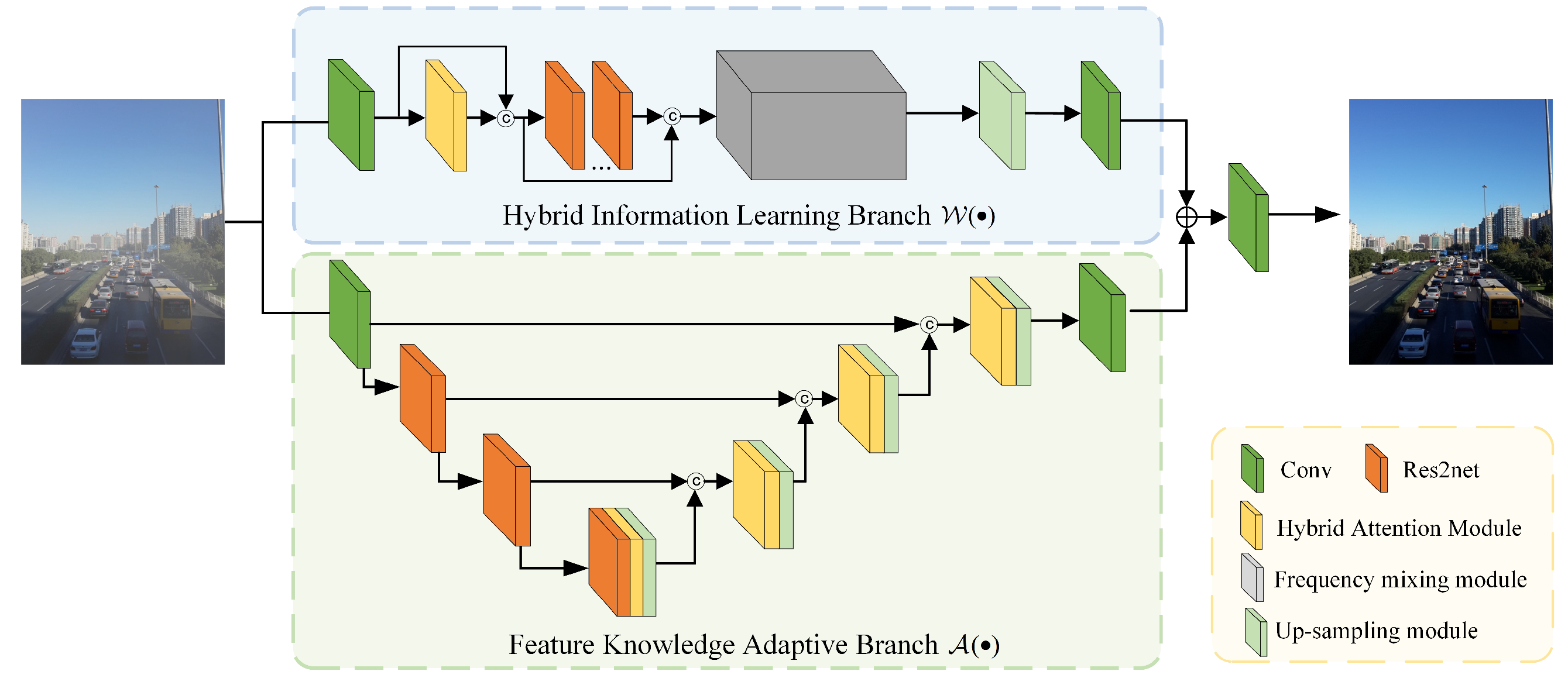
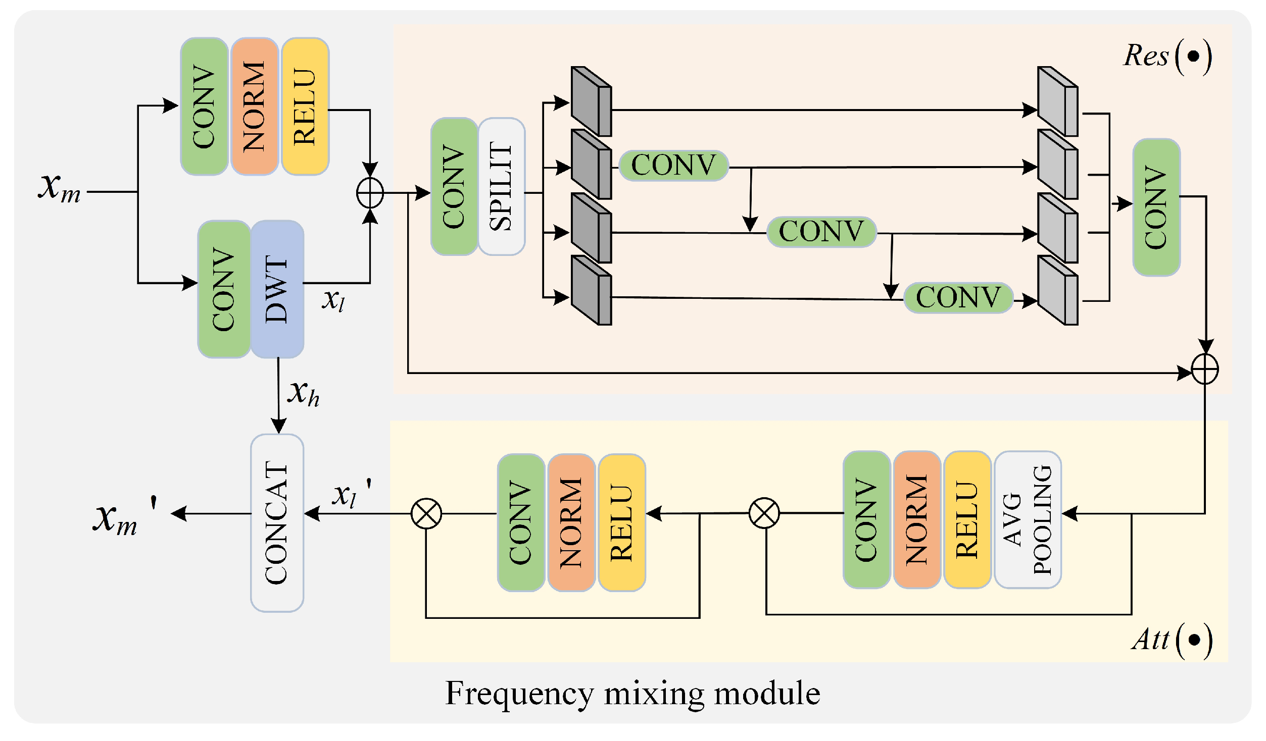
3.1. Dual-Branch Wavelet Transform Network
3.1.1. Hybrid Information-Learning Branch
3.1.2. Feature-Knowledge Adaptive Branch
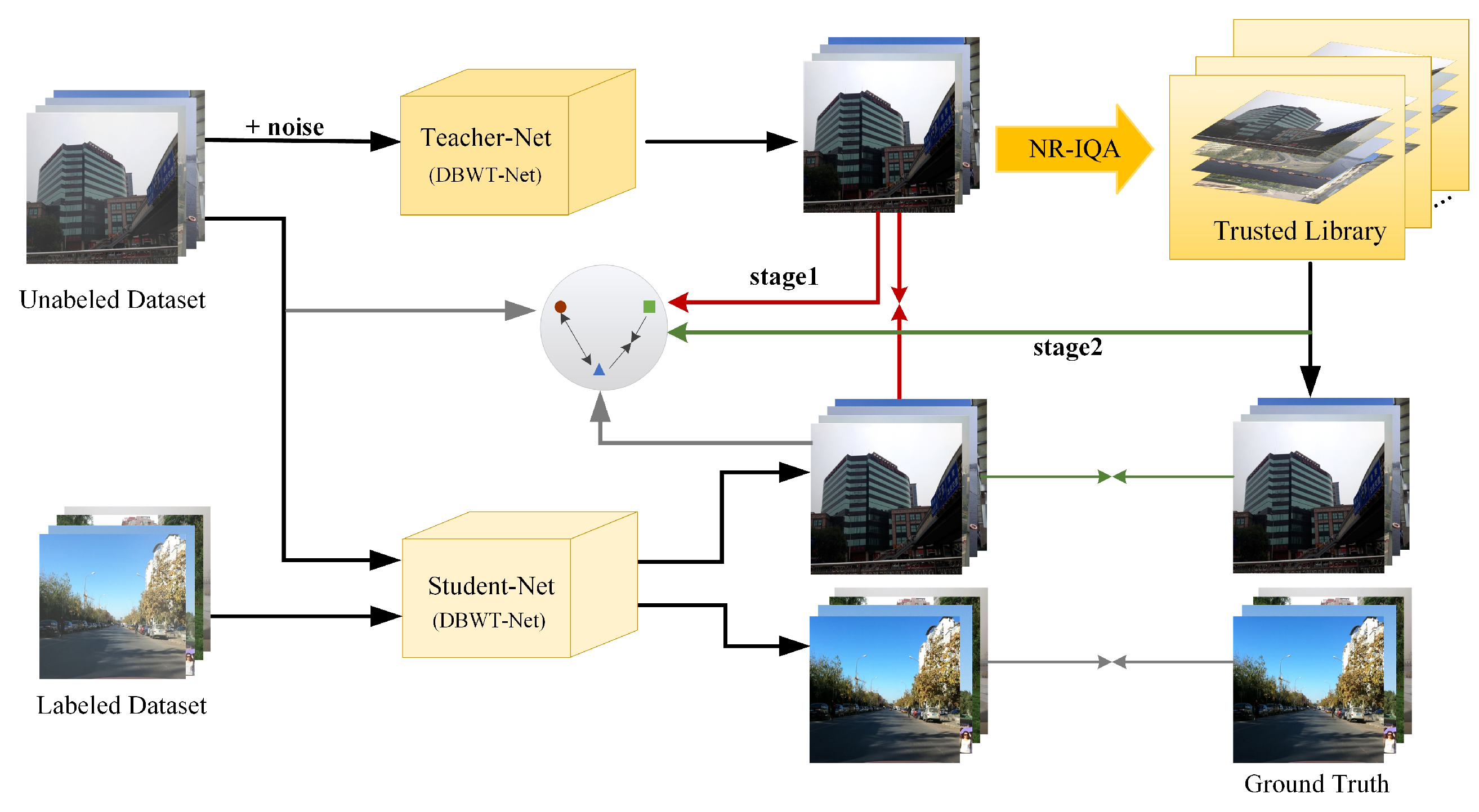
3.2. Semi-Supervised Image-Dehazing Network Based on a Trusted Library
3.2.1. Teacher–Student Model
3.2.2. Trusted Library
3.3. Loss Function
3.3.1. Supervised Loss
3.3.2. Unsupervised Loss
4. Experiments
4.1. Implementation Details
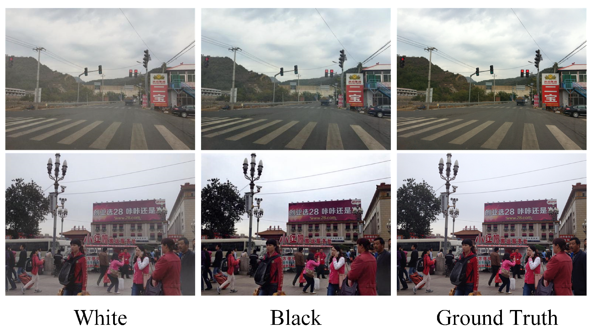
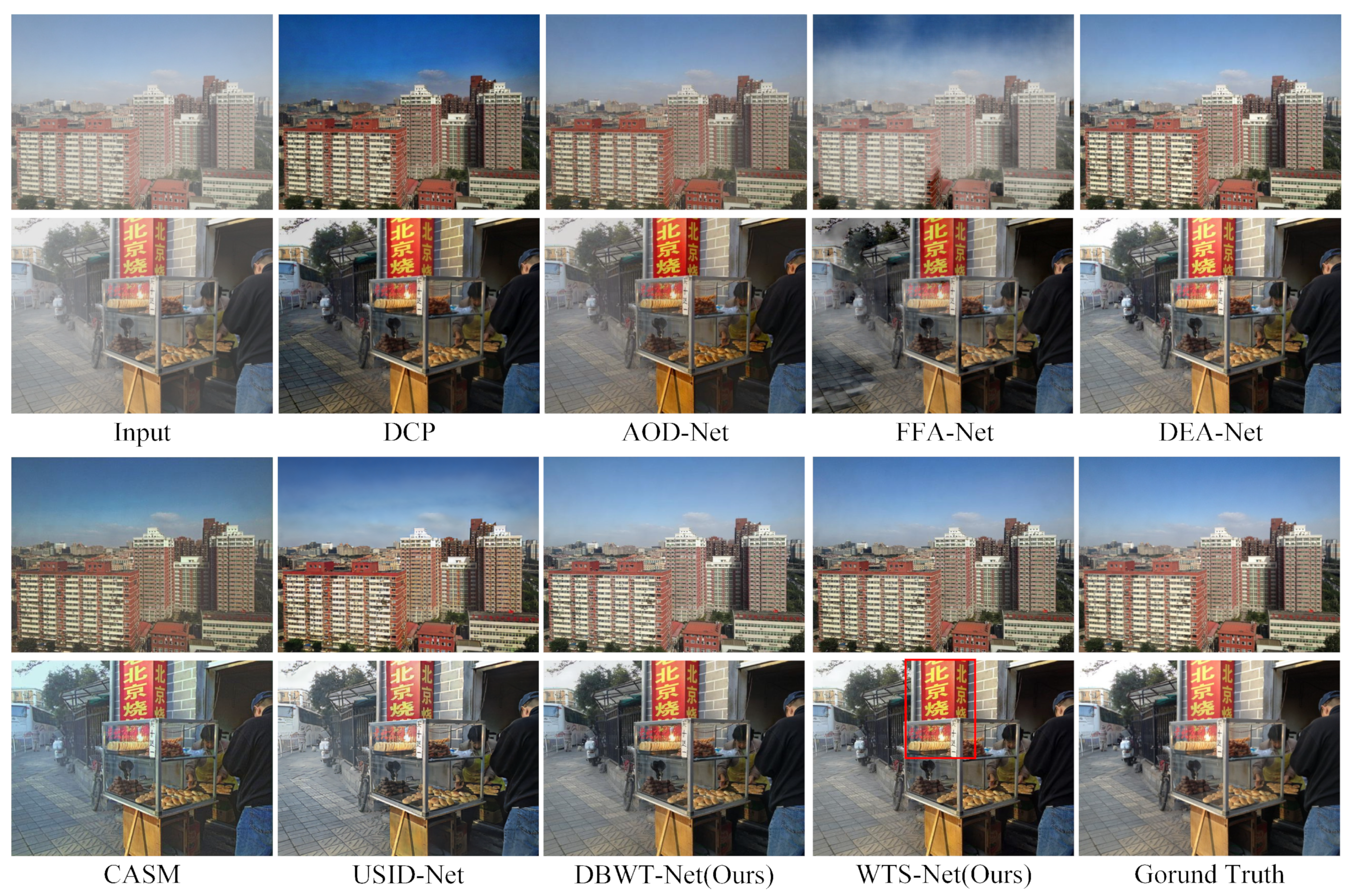
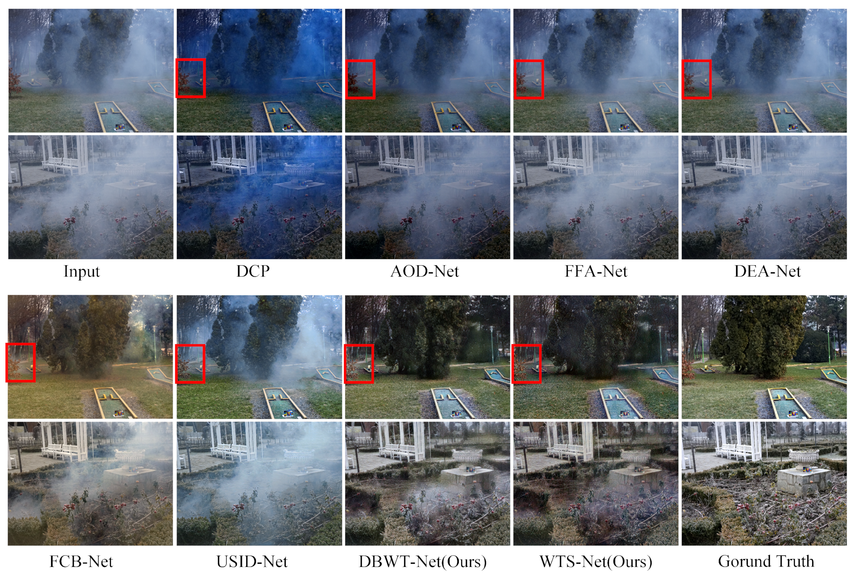
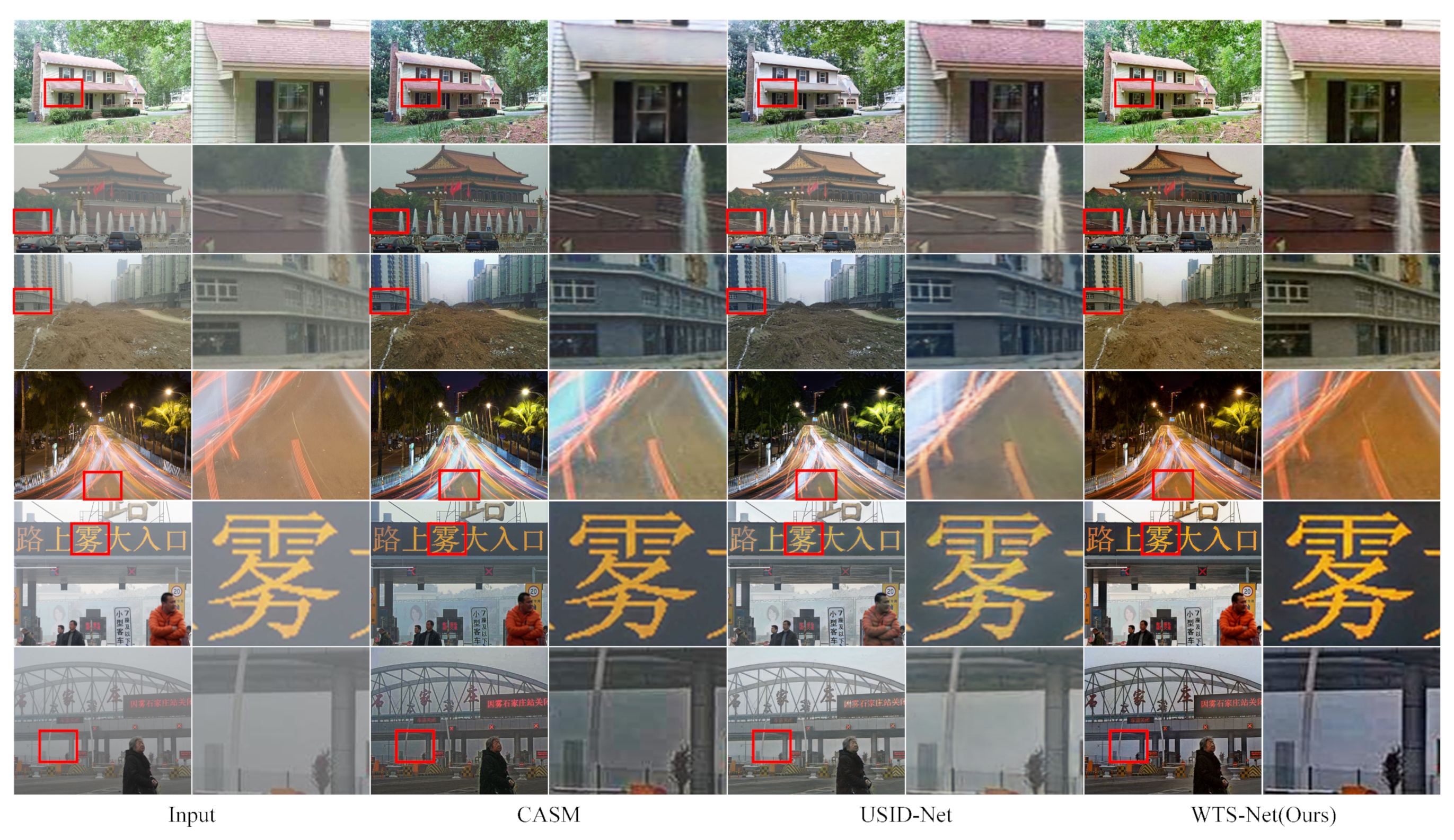
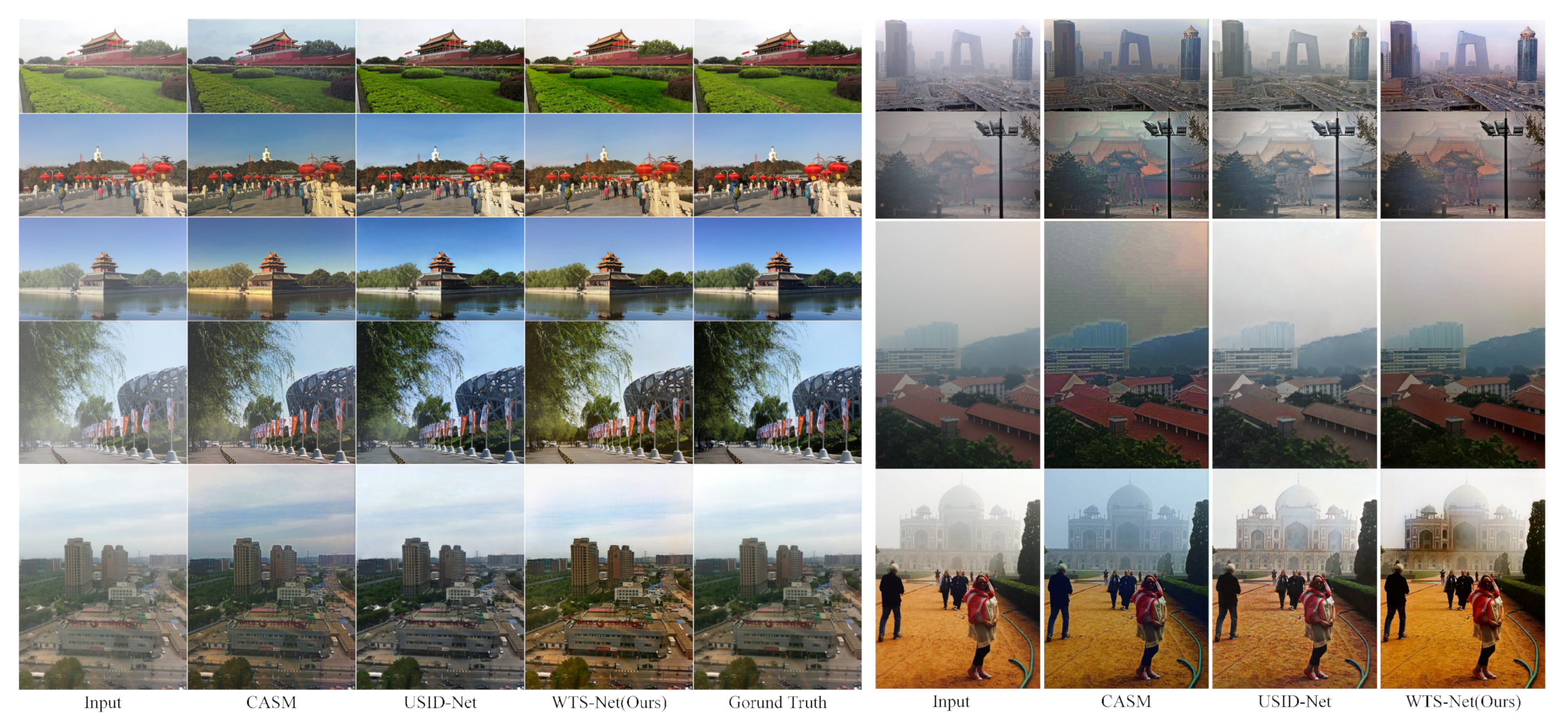
4.2. Supervised Dataset Evaluation
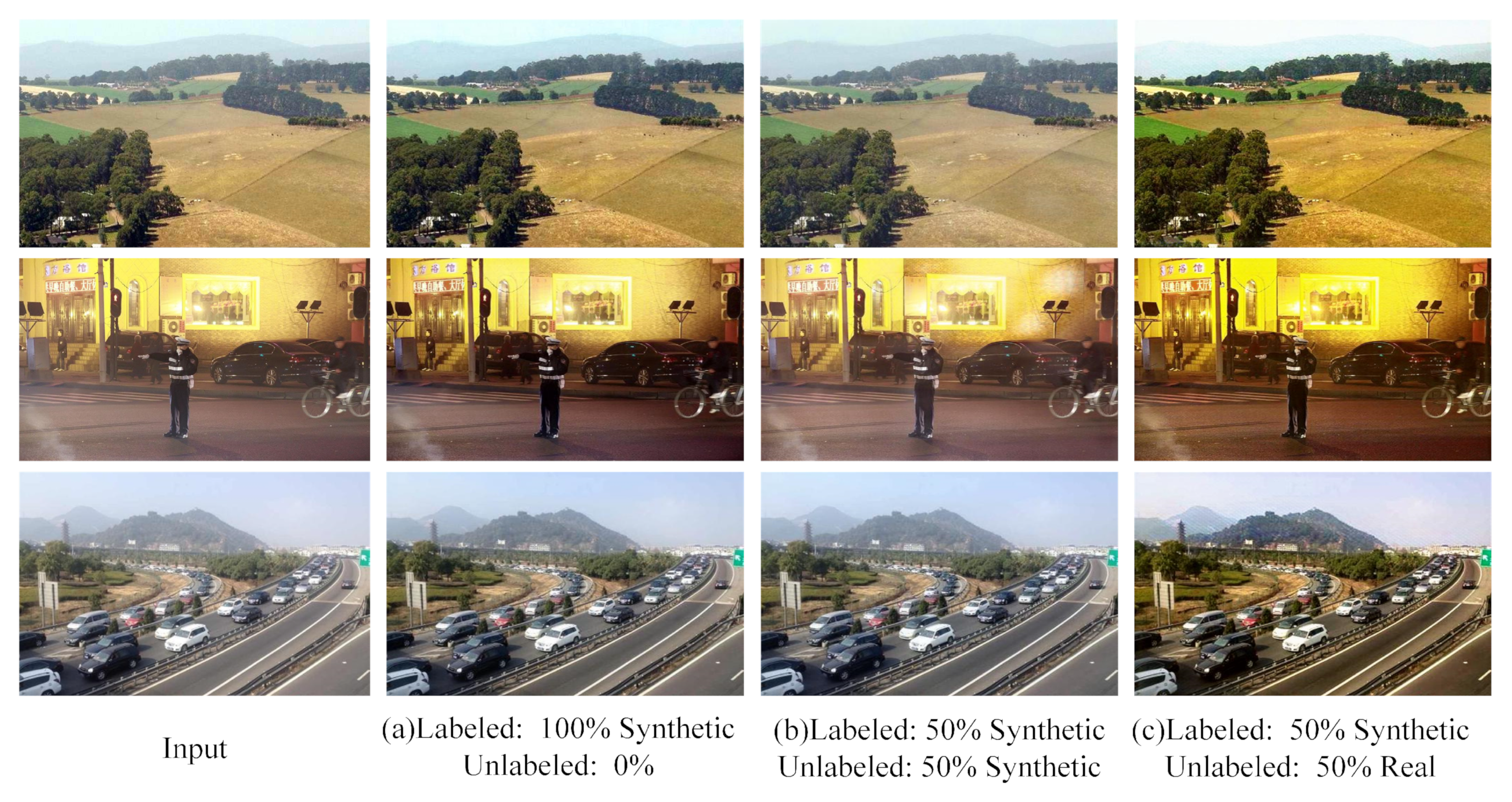
4.3. Unsupervised Dataset Evaluation
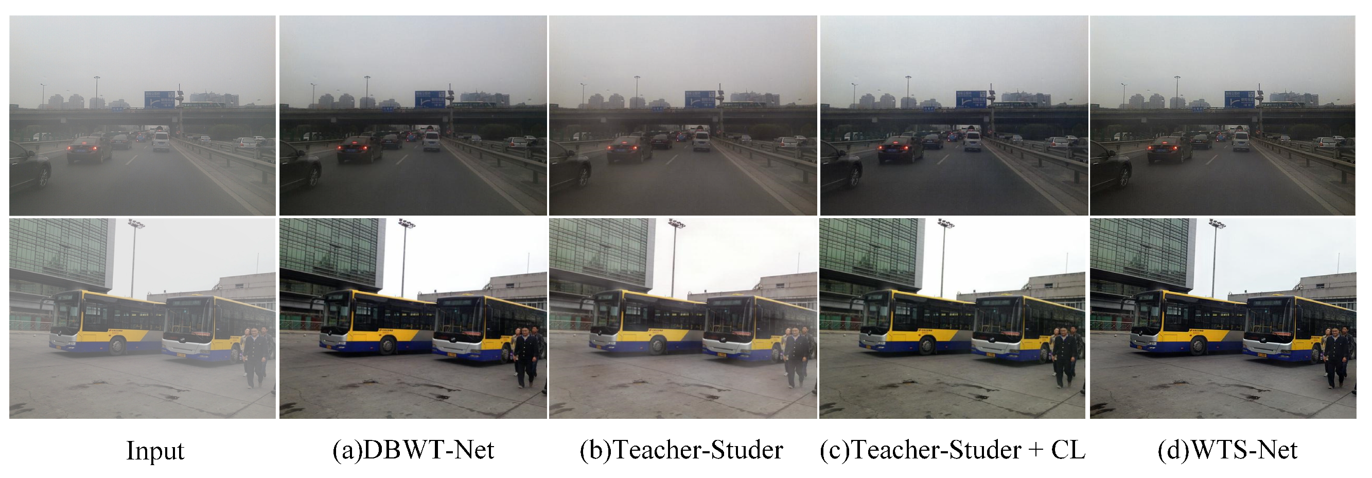
4.4. Ablation Study
5. Conclusions
Author Contributions
Funding
Data Availability Statement
Conflicts of Interest
References
- He, K.; Sun, J.; Tang, X. Single image haze removal using dark channel prior. IEEE Trans. Pattern Anal. Mach. Intell. 2010, 33, 2341–2353. [Google Scholar] [CrossRef] [PubMed]
- Berman, D.; Avidan, S. Non-local image dehazing. In Proceedings of the IEEE Conference on Computer Vision and Pattern Recognition, Las Vegas, NV, USA, 27–30 June 2016. [Google Scholar]
- Zhu, Q.; Mai, J.; Shao, L. A fast single image haze removal algorithm using color attenuation prior. IEEE Trans. Image Process. 2015, 24, 3522–3533. [Google Scholar] [CrossRef] [PubMed]
- Li, B.; Peng, X.; Wang, Z.; Xu, J.; Feng, D. Aod-net: All-in-one dehazing network. In Proceedings of the IEEE International Conference on Computer Vision, Venice, Italy, 22–29 October 2017; pp. 4770–4778. [Google Scholar]
- Cai, B.; Xu, X.; Jia, K.; Qing, C.; Tao, D. Dehazenet: An end-to-end system for single image haze removal. IEEE Trans. Image Process. 2016, 25, 5187–5198. [Google Scholar] [CrossRef] [PubMed]
- Qin, X.; Wang, Z.; Bai, Y.; Xie, X.; Jia, H. FFA-Net: Feature fusion attention network for single image dehazing. Aaai Conf. Artif. Intell. 2020, 34, 11908–11915. [Google Scholar] [CrossRef]
- Wu, H.; Qu, Y.; Lin, S.; Zhou, J.; Qiao, R.; Zhang, Z.; Ma, L. Contrastive learning for compact single image dehazing. In Proceedings of the IEEE/CVF Conference on Computer Vision and Pattern Recognition, Nashville, TN, USA, 19–25 June 2021; pp. 10551–10560. [Google Scholar]
- Guo, C.L.; Yan, Q.; Anwar, S.; Cong, R.; Ren, W.; Li, C. Image dehazing transformer with transmission-aware 3d position embedding. In Proceedings of the IEEE/CVF Conference on Computer Vision and Pattern Recognition, New Orleans, LA, USA, 18–24 June 2022; pp. 5812–5820. [Google Scholar]
- Li, Y.; Miao, Q.; Ouyang, W.; Ma, Z.; Fang, H.; Dong, C.; Quan, Y. LAP-Net: Level-aware progressive network for image dehazing. In Proceedings of the IEEE/CVF International Conference on Computer Vision, Seoul, Republic of Korea, 27 October–2 November 2019; pp. 3276–3285. [Google Scholar]
- Zhang, Y.; Zhou, S.; Li, H. Depth information assisted collaborative mutual promotion network for single image dehazing. In Proceedings of the IEEE/CVF Conference on Computer Vision and Pattern Recognition, Seattle, WA, USA, 16–22 June 2024; pp. 2846–2855. [Google Scholar]
- Guo, T.; Mousavi, H.S.; Vu, T.H.; Monga, V. Deep wavelet prediction for image super-resolution. In Proceedings of the IEEE Conference on Computer Vision and Pattern Recognition Workshops, Honolulu, HI, USA, 21–26 July 2017; pp. 104–113. [Google Scholar]
- Liu, P.; Zhang, H.; Zhang, K.; Lin, L.; Zuo, W. Multi-level wavelet-CNN for image restoration. In Proceedings of the IEEE Conference on Computer Vision and Pattern Recognition Workshops, Salt Lake City, UT, USA, 18–22 June 2018; pp. 773–782. [Google Scholar]
- Fu, M.; Liu, H.; Yu, Y.; Chen, J.; Wang, K. Dw-gan: A discrete wavelet transform gan for nonhomogeneous dehazing. In Proceedings of the IEEE/CVF Conference on Computer Vision and Pattern Recognition, Nashville, TN, USA, 19–25 June 2021; pp. 203–212. [Google Scholar]
- Li, L.; Dong, Y.; Ren, W.; Pan, J.; Gao, C.; Sang, N.; Yang, M.H. Semi-supervised image dehazing. IEEE Trans. Image Process. 2019, 29, 2766–2779. [Google Scholar] [CrossRef] [PubMed]
- Tarvainen, A.; Valpola, H. Mean teachers are better role models: Weight-averaged consistency targets improve semi-supervised deep learning results. arXiv 2017, arXiv:1703.01780. [Google Scholar]
- Hinton, G.; Vinyals, O.; Dean, J. Distilling the knowledge in a neural network. arXiv 2015, arXiv:1503.02531. [Google Scholar]
- Lee, S.; Jang, D.; Kim, D.S. Temporally averaged regression for semi-supervised low-light image enhancement. In Proceedings of the IEEE/CVF Conference on Computer Vision and Pattern Recognition, Vancouver, BC, Canada, 18–22 June 2023; pp. 4208–4217. [Google Scholar]
- Huang, S.; Wang, K.; Liu, H.; Chen, J.; Li, Y. Contrastive semi-supervised learning for underwater image restoration via reliable bank. In Proceedings of the IEEE/CVF Conference on Computer Vision and Pattern Recognition, Vancouver, BC, Canada, 18–22 June 2023; pp. 18145–18155. [Google Scholar]
- Zhang, H.; Patel, V.M. Densely connected pyramid dehazing network. In Proceedings of the IEEE Conference on Computer Vision and Pattern Recognition, Salt Lake City, UT, USA, 18–22 June 2018; pp. 3194–3203. [Google Scholar]
- Cong, X.; Gui, J.; Zhang, J.; Hou, J.; Shen, H. A semi-supervised nighttime dehazing baseline with spatial-frequency aware and realistic brightness constraint. In Proceedings of the IEEE/CVF Conference on Computer Vision and Pattern Recognition, Seattle, WA, USA, 16–22 June 2024; pp. 2631–2640. [Google Scholar]
- Wang, W.; Yang, H.; Fu, J.; Liu, J. Zero-reference low-light enhancement via physical quadruple priors. In Proceedings of the IEEE/CVF Conference on Computer Vision and Pattern Recognition, Seattle, WA, USA, 16–22 June 2024; pp. 26057–26066. [Google Scholar]
- Duong, M.T.; Lee, S.; Hong, M.C. DMT-Net: Deep multiple networks for low-light image enhancement based on retinex model. IEEE Access 2023, 11, 132147–132161. [Google Scholar] [CrossRef]
- Li, B.; Ren, W.; Fu, D.; Tao, D.; Feng, D.; Zeng, W.; Wang, Z. Benchmarking single-image dehazing and beyond. IEEE Trans. Image Process. 2018, 28, 492–505. [Google Scholar] [CrossRef] [PubMed]
- Ying, Z.; Niu, H.; Gupta, P.; Mahajan, D.; Ghadiyaram, D.; Bovik, A. From patches to pictures (PaQ-2-PiQ): Mapping the perceptual space of picture quality. In Proceedings of the IEEE/CVF Conference on Computer Vision and Pattern Recognition, Seattle, WA, USA, 14–19 June 2020; pp. 3575–3585. [Google Scholar]
- Wang, J.; Chan, K.C.; Loy, C.C. Exploring clip for assessing the look and feel of images. Aaai Conf. Artif. Intell. 2023, 37, 555–2563. [Google Scholar] [CrossRef]
- Ke, J.; Wang, Q.; Wang, Y.; Milanfar, P.; Yang, F. Musiq: Multi-scale image quality transformer. In Proceedings of the IEEE/CVF International Conference on Computer Vision, Montreal, BC, Canada, 11–17 October 2021; pp. 5148–5157. [Google Scholar]
- Zhang, W.; Kede, M.; Yan, J.; Deng, D.; Wang, Z. Blind Image Quality Assessment Using a Deep Bilinear Convolutional Neural Network. IEEE TRansactions Circuits Syst. Video Technol. 2020, 30, 36–47. [Google Scholar] [CrossRef]
- Mittal, A.; Soundararajan, R.; Bovik, A.C. Making a completely blind image quality analyzer. IEEE Signal Process. Lett. 2012, 20, 209–212. [Google Scholar] [CrossRef]
- Mittal, A.; Moorthy, A.K.; Bovik, A.C. No-reference image quality assessment in the spatial domain. IEEE Trans. Image Process. 2012, 21, 4695–4708. [Google Scholar] [CrossRef] [PubMed]
- Zhang, L.; Zhang, L.; Bovik, A.C. A feature-enriched completely blind image quality evaluator. IEEE Trans. Image Process. 2015, 24, 2579–2591. [Google Scholar] [CrossRef] [PubMed]
- Kang, L.; Ye, P.; Li, Y.; Doermann, D. Convolutional neural networks for no-reference image quality assessment. In Proceedings of the IEEE Conference on Computer Vision and Pattern Recognition, Columbus, OH, USA, 23–28 June 2014; pp. 1733–1740. [Google Scholar]
- Ancuti, C.O.; Ancuti, C.; Timofte, R. NH-HAZE: An image dehazing benchmark with non-homogeneous hazy and haze-free images. In Proceedings of the IEEE/CVF Conference on Computer Vision and Pattern Recognition Workshops, Seattle, WA, USA, 14–19 June 2020; pp. 444–445. [Google Scholar]
- Chen, Z.; He, Z.; Lu, Z.M. DEA-Net: Single image dehazing based on detail-enhanced convolution and content-guided attention. IEEE Trans. Image Process. 2024, 33, 1002–1015. [Google Scholar] [CrossRef] [PubMed]
- Wang, J.; Wu, S.; Yuan, Z.; Tong, Q.; Xu, K. Frequency compensated diffusion model for real-scene dehazing. Neural Netw. 2024, 175, 106281. [Google Scholar] [CrossRef] [PubMed]
- Wang, X.; Chen, X.A.; Ren, W.; Han, Z.; Fan, H.; Tang, Y.; Liu, L. Compensation atmospheric scattering model and two-branch network for single image dehazing. IEEE Trans. Emerg. Top. Comput. Intell. 2024, 8, 2880–2896. [Google Scholar] [CrossRef]
- Li, J.; Li, Y.; Zhuo, L.; Kuang, L.; Yu, T. USID-Net: Unsupervised single image-dehazing network via disentangled representations. IEEE Trans. Multimed. 2022, 25, 3587–3601. [Google Scholar] [CrossRef]

| Method | SOTS-Outdoor | NH-Haze | ||
|---|---|---|---|---|
| SSIM | PSNR | SSIM | PSNR | |
| DCP | 0.815 | 19.13 | 0.520 | 10.57 |
| AOD-Net | 0.927 | 20.08 | 0.569 | 15.40 |
| FFA-Net | 0.984 | 33.57 | 0.692 | 19.87 |
| DEA-Net | 0.980 | 31.68 | - | - |
| FCB-Net | 0.958 | 28.19 | 0.622 | 14.16 |
| CASM | 0.873 | 19.87 | 0.532 | 13.33 |
| USID-Net | 0.919 | 23.89 | 0.556 | 13.21 |
| DBWT-Net (Ours) | 0.974 | 30.59 | 0.741 | 20.34 |
| WTS-Net (Ours) | 0.961 | 28.47 | 0.677 | 19.64 |
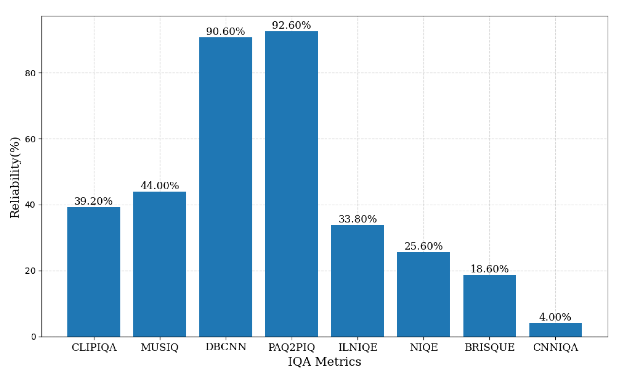
| Method | CLIPIQA ↑ | MUSIQ ↑ | DBCNN ↑ | NIQE ↓ |
|---|---|---|---|---|
| CASM | 0.4460 | 58.2828 | 0.4665 | 4.3039 |
| USID-Net | 0.4793 | 58.6729 | 0.4678 | 3.8499 |
| WTS-Net (Ours) | 0.4470 | 58.7700 | 0.5071 | 4.5336 |
| Method | Synthetic Images | Real Images | ||||
|---|---|---|---|---|---|---|
| SSIM | PSNR | CLIPIQA ↑ | MUSIQ ↑ | DBCNN ↑ | NIQE ↓ | |
| CASM | 0.8801 | 28.1852 | 0.5457 | 65.9068 | 0.5449 | 3.5975 |
| USID | 0.8033 | 29.5860 | 0.5762 | 65.2448 | 0.5141 | 3.4019 |
| WTS-Net (Ours) | 0.8704 | 29.3823 | 0.5978 | 65.7613 | 0.5705 | 3.2224 |
| TS | CL | TL | PSNR | SSIM | |
|---|---|---|---|---|---|
| DBWT-Net | 26.515 | 0.939 | |||
| Teacher–Student | ✓ | 24.384 | 0.901 | ||
| Teacher–Student + CL | ✓ | ✓ | 24.922 | 0.929 | |
| WTS-Net | ✓ | ✓ | ✓ | 25.605 | 0.935 |
Disclaimer/Publisher’s Note: The statements, opinions and data contained in all publications are solely those of the individual author(s) and contributor(s) and not of MDPI and/or the editor(s). MDPI and/or the editor(s) disclaim responsibility for any injury to people or property resulting from any ideas, methods, instructions or products referred to in the content. |
© 2025 by the authors. Licensee MDPI, Basel, Switzerland. This article is an open access article distributed under the terms and conditions of the Creative Commons Attribution (CC BY) license (https://creativecommons.org/licenses/by/4.0/).
Share and Cite
Li, W.; Chang, C. Semi-Supervised Image-Dehazing Network Based on a Trusted Library. Electronics 2025, 14, 2956. https://doi.org/10.3390/electronics14152956
Li W, Chang C. Semi-Supervised Image-Dehazing Network Based on a Trusted Library. Electronics. 2025; 14(15):2956. https://doi.org/10.3390/electronics14152956
Chicago/Turabian StyleLi, Wan, and Chenyang Chang. 2025. "Semi-Supervised Image-Dehazing Network Based on a Trusted Library" Electronics 14, no. 15: 2956. https://doi.org/10.3390/electronics14152956
APA StyleLi, W., & Chang, C. (2025). Semi-Supervised Image-Dehazing Network Based on a Trusted Library. Electronics, 14(15), 2956. https://doi.org/10.3390/electronics14152956