Convex Optimization-Based Constrained Trajectory Planning for Autonomous Vehicles

Abstract

This paper proposes a constrained trajectory optimization framework for autonomous vehicles (AVs) based on convex programming techniques. An enhanced kinematic vehicle model is introduced to capture dynamic motion characteristics that are often overlooked in conventional models. For obstacle avoidance, environmental constraints are transformed into convex formulations using free-space corridor methods. The trajectory planning process is further optimized through a linearized model predictive control (MPC) scheme, which considers both vehicle dynamics and environmental safety. The resulting formulation enables efficient convex optimization suitable for real-time implementation. Experimental results in various scenarios demonstrate improvements in both trajectory smoothness and safety. Furthermore, the proposed optimization method reduces the average execution time by nearly 70% compared to the nonlinear alternative, validating its computational efficiency and practical applicability.

1. Introduction

Autonomous driving technology has made remarkable strides in both academia and industry, expanding its applications from highway scenarios to increasingly complex urban environments [1], as illustrated in Figure 1. Compared to highway scenarios, urban driving involves denser and more dynamic environments, including pedestrians, cyclists, and vehicles. These agents often behave unpredictably, significantly complicating trajectory planning tasks [2]. Increasing attention is being paid to modeling interactions with dynamic agents through intention-aware predictors, game-theoretic formulations, or learned behavior models. Additionally, the irregular shape of the ego vehicle creates nonlinear constraints for the collision avoidance task, which further complicates the planning problem. Thus, effective urban trajectory planning is critical for ensuring safety, ride comfort, and overall efficiency. Specifically, the planner must simultaneously manage complex vehicle dynamics and real-time obstacle avoidance with limited computational resources. To this end, modern approaches are exploring strategies such as sequential convex programming (SCP), hybrid convex–non-convex formulations, and adaptive receding horizon planning to improve flexibility under non-convex constraints.

The primary aim of this paper is to address these challenges by introducing a novel convex optimization framework for trajectory planning, specifically tailored to urban driving environments. We propose an enhanced vehicle kinematic model that integrates acceleration and steering dynamics, providing a more realistic representation of vehicle motion. Additionally, we present a robust method to construct convex feasible areas through spatial corridor techniques, effectively simplifying the obstacle avoidance problem into manageable convex constraints. Our method formulates the trajectory planning problem as a constrained quadratic programming (QP) task within a linearized model predictive control (MPC) framework, enabling efficient and reliable solutions even in dynamic environments. By using a discretized enhanced kinematic bicycle model, the system achieves accurate state prediction while remaining computationally efficient. The spatial corridors tightly constrain the vehicle within a safe navigable space, while soft constraints further enhance passenger comfort by allowing flexibility to maintain distances from obstacles. The main contributions of this work include the following:

• A comprehensive derivation and analysis of an enhanced kinematic bicycle model that includes acceleration and steering dynamics;
• A robust and practical obstacle avoidance strategy designed for complex urban environments, ensuring robust safety and feasibility;
• Implementation and validation of a real-time convex optimization framework within a linearized MPC structure, supported by extensive simulation experiments.

2. Related Work

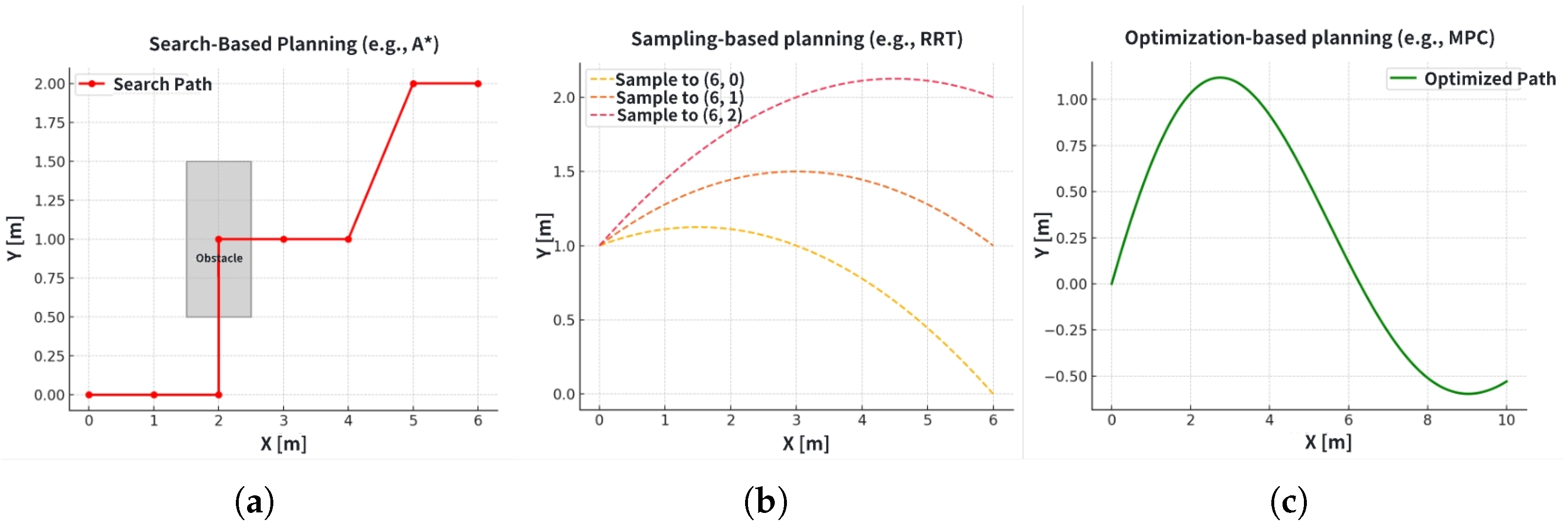
The trajectory planning methods are typically classified into three categories: search-based, sampling-based, and optimization-based planning, as illustrated in Figure 2. Search-based algorithms [3,4,5] discretize the environment and perform graph-based searches to identify feasible paths. Nevertheless, due to their coarse resolution and computational cost, these methods are typically applied in unstructured or low-speed scenarios, such as parking [6]. The sampling-based approaches [7,8], on the other hand, sample multiple candidate trajectories by selecting a range of target points and generating corresponding paths. The corresponding paths are generated using predefined curve models, such as polynomial curves or Bézier curves. Each trajectory is evaluated using a cost function, and the one with the highest score is selected as the output. However, the performance of these sampling-based methods depends heavily on sampling density and curve models, and is limited by the state space coverage. They also face challenges in handling dynamic obstacles and real-time constraints. In contrast, the optimization-based trajectory planning [9,10] is a more advanced approach. This approach directly formulates the trajectory generation problem as a numerical optimization problem, where the vehicle’s future states serve as optimization variables. These methods are well-suited for complex urban environments as they can incorporate detailed safety non-convex constraints such as obstacle avoidance [11]. Additionally, they produce flexible and smooth trajectories while maintaining computational efficiency.

Obstacle avoidance strategies generally fall into two categories: potential field-based and spatial corridor-based methods. Potential field methods treat the vehicle as if it is moving within a virtual force field [12,13]. These methods are computationally efficient but often struggle with sensitivity to parameter tuning and may perform poorly in cluttered environments. While this approach is intuitive and lightweight, it is less suitable for handling road boundaries. This is because potential fields model obstacles as repulsive points or regions, which works well for discrete obstacles but is less effective for continuous features like road boundaries. Unlike obstacles, road boundaries do not simply act as barriers to avoid; they define a navigable corridor. When these continuous lane boundaries are modeled as repulsive forces, it can lead to unnatural or oscillatory behavior, particularly near the edges of the road. In contrast, spatial corridor methods define safe navigation zones, which enable dynamically feasible trajectories. These trajectories are better aligned with the vehicle’s kinematic constraints [14,15]. These methods leverage environmental information to construct the corridors, ensuring a safer and more efficient navigation process. However, it is equally important to implement an effective scheme for constructing these corridors, ensuring the safety and adaptability to changing road conditions. Some previous studies generated corridors using a predefined expansion order and constant size, which were inadequate and often struggled with curved roads featuring large curvatures [16].

The trajectory planning problem can be approached in either the Cartesian coordinate system through spatio-temporal planning [17] or in the Frenet frame using path-speed decoupling [18,19]. The Cartesian approach provides high accuracy for both vehicle kinematics and environment modeling, while the Frenet frame leverages road reference lines to simplify path representation [20].

Table 1. Comparison of Cartesian and Frenet frames for trajectory planning.

Aspect	Cartesian Frame	Frenet Frame
Coordinate Definition	$x,y$	s (longitudinal), l (lateral)
Reference	Global map frame	Relative to a centerline
Trajectory Representation	Direct position in 2D space	Longitudinal progression and lateral deviation
Obstacle Modeling	Obstacles described globally	Projected into path-relative coordinates
Kinematic Modeling	Accurate but typically nonlinear	Simplified under path-aligned assumptions
Optimization Complexity	Higher due to coupling of x, y	Lower due to path-speed decoupling
Preferred Scenarios	Complex or unstructured environments	Structured roads with clear lane geometry

summarizes the differences between Cartesian and Frenet coordinate systems. Both methods typically start with an initial coarse solution, followed by optimization for smoothness [21]. A good initial guess can significantly accelerate convergence in numerical optimization.

Recent research has focused on reformulating trajectory planning problems as convex optimization problems. Prior studies have shown that such problems can be cast as quadratic programming (QP) problems [22,23], incorporating obstacle avoidance as linear constraints. However, the following key challenges remain: (1) efficiently and accurately generating collision-free trajectories in environments with dense and unknown obstacles; (2) optimizing the computational efficiency and robustness within the constraints of limited computing resources; (3) improving the feasibility and flexibility of trajectory generation without sacrificing safety or integrity.

The rest of the paper is organized as follows: Section 3 introduces the proposed kinematic model. Section 4 details the trajectory planning method. Section 5 presents the experimental results. Finally, Section 6 summarizes the paper and draws conclusions.

3. Proposed Vehicle Kinematics

In this section, we adopt an extended bicycle model to describe vehicle motion, incorporating acceleration and steering for higher fidelity. The vehicle’s state is denoted by position ($x,y$), heading angle $\theta$, and velocity v, while control inputs include acceleration a and front wheel angle $\delta$. The simplified model can be expressed as follows:

$$\left\{\begin{array}{c}\dot{x}=vcos\theta \\ \dot{y}=vsin\theta \\ \dot{\theta }={\displaystyle \frac{vtan\delta }{L}}\\ \dot{v}=a\end{array},\right.$$

(1)

where L represents the wheelbase of the vehicle, as shown in Figure 3.

One could use a differentially flat vehicle model [24] considering the flat output [25], represented as follows:

$$\left\{\begin{array}{c}v=\sqrt{{\dot{x}}^2+{\dot{y}}^2}={\left({\dot{\ell }}^T\dot{\ell }\right)}^{1/2}\\ \theta =arctan2\left(\dot{y},\dot{x}\right)\\ a=\left(\dot{x}\ddot{x}+\dot{y}\ddot{y}\right)/\sqrt{{\dot{x}}^2+{\dot{y}}^2}={\displaystyle \frac{\left({\ddot{\ell }}^T\dot{\ell }\right)}{{\left({\dot{\ell }}^T\dot{\ell }\right)}^{1/2}}}\\ \delta =arctan\left(\left(\dot{x}\ddot{y}-\dot{y}\ddot{x}\right)L/{\left({\dot{x}}^2+{\dot{y}}^2\right)}^{3/2}\right)=arctan\left({\displaystyle \frac{{\ddot{\ell }}^T\mathbf{B}\dot{\ell }·L}{{\left({\dot{\ell }}^T\dot{\ell }\right)}^{3/2}}}\right)\end{array},\right.$$

(2)

where $\ell :=(x,y)$ is the flat output; that is, vehicle position. $B:=[0,-1;1,0]$ is an auxiliary antisymmetric matrix. When the velocity is small, variables such as acceleration and front wheel angle are undefined and therefore uncontrollable, that is, a singularity configuration issue. However, more often than in the real world, we come across the situation where the vehicle is at a very low speed.

In the model of Equation (1), there is a delay between the control input and the vehicle state; that is, not all states are directly controlled by the control input. To model motion more accurately, the vehicle is assumed to follow an arc during a discrete time interval. The center of the rotation $(C_x,C_y)$ and rotation radius R are derived accordingly.

$$\left\{\begin{array}{c}{C}_x=x-Rsin\theta \\ C_y=y+Rcos\theta \\ R={\displaystyle \frac{L}{tan\delta }}\end{array}.\right.$$

(3)

Using the displacement $\Delta s$, the corresponding rotation angle $\Delta \theta$ is calculated:

$$\Delta s=v\Delta t+{\displaystyle \frac{a\Delta t^2}{2}},$$

(4)

$$\Delta \theta ={\displaystyle \frac{\Delta s}{R}}=\left(v\Delta t+{\displaystyle \frac{a\Delta t^2}{2}}\right){\displaystyle \frac{tan\delta }{L}}.$$

(5)

So, the vehicle’s future position $(x^{\prime },y^{\prime })$ is predicted:

$$\left\{\begin{array}{c}{x}^{\prime }=C_x+Rsin(\theta +\Delta \theta )\\ y^{\prime }=C_y-Rcos(\theta +\Delta \theta )\end{array}.\right.$$

(6)

Substituting Equation (3) and Equation (5) into the position update equations in Equation (6) yields the following form of new state $(x^{\prime },y^{\prime },{\theta }^{\prime },v^{\prime })$:

$$\left\{\begin{array}{c}{x}^{\prime }=x-Rsin\theta +Rsin(\theta +\Delta \theta )=x-L{\displaystyle \frac{sin\theta }{tan\delta }}+L{\displaystyle \frac{sin(\theta +\frac{v\Delta t+0.5a\Delta t^2}{L}tan\delta )}{tan\delta }}\\ y^{\prime }=y+Rcos\theta -Rcos(\theta +\Delta \theta )=y+L{\displaystyle \frac{cos\theta }{tan\delta }}-L{\displaystyle \frac{cos(\theta +\frac{v\Delta t+0.5a\Delta t^2}{L}tan\delta )}{tan\delta }}\\ {\theta }^{\prime }=\theta +(v\Delta t+{\displaystyle \frac{a\Delta t^2}{2}}){\displaystyle \frac{tan\delta }{L}}\\ v^{\prime }=v+a\Delta t\end{array}.\right.$$

(7)

Equation (7) represents a discretized update model for the vehicle’s state. We approximate the differential form of the state change $(\dot{x},\dot{y},\dot{\theta },\dot{v})$ with respect to time by taking the first-order difference over the sampling interval $\Delta t$:

$$\left\{\begin{array}{c}\dot{x}=(v+a\Delta t)cos(\theta +{\displaystyle \frac{v\Delta t+0.5a\Delta t^2}{L}}tan\delta )\\ \dot{y}=(v+a\Delta t)sin(\theta +{\displaystyle \frac{v\Delta t+0.5a\Delta t^2}{L}}tan\delta )\\ \dot{\theta }=(v+a\Delta t){\displaystyle \frac{tan\delta }{L}}\\ \dot{v}=a\end{array}.\right.$$

(8)

This model takes into account the impact of the vehicle’s control input on its velocity, position, and direction. These formulas can be effectively used to describe the dynamic behavior of the vehicle over a given period of time. The new model provides higher accuracy by incorporating the effects of acceleration and steering, suitable for applications requiring high dynamic accuracy. A more compact form of the kinematic model is the following:

$$\dot{\mathbf{x}}=\mathit{f}(\mathbf{x},\mathbf{u}),$$

(9)

where $\mathbf{x}=(x,y,\theta ,v)$ describes the configuration of the center of the rear wheels, and $\mathbf{u}=(a,\delta )$ is the control input. For a given reference trajectory, each point $({\mathbf{x}}_{ref},{\mathbf{u}}_{ref})$ also satisfies the kinematic equations. Therefore, its trajectory is expressed by the following formula:

$${\dot{\mathbf{x}}}_{ref}=\mathit{f}({\mathbf{x}}_{ref},{\mathbf{u}}_{ref}).$$

(10)

The reference points are generated from a coarse trajectory produced by the hybrid A* algorithm. This trajectory is sampled and smoothed to yield the nominal motion plan, which serves as the baseline for linearization in the MPC optimization. Expanding the right side of Equation (9) around the reference point using Taylor series and discarding the higher-order terms yields the following:

$$\dot{\mathbf{x}}=\mathit{f}({\mathbf{x}}_{ref},{\mathbf{u}}_{ref})+{\displaystyle \frac{\partial \mathit{f}}{\partial \mathbf{x}}}(\mathbf{x}-{\mathbf{x}}_{ref})+{\displaystyle \frac{\partial \mathit{f}}{\partial \mathbf{u}}}(\mathbf{u}-{\mathbf{u}}_{ref}),$$

(11)

where ${\displaystyle \frac{\partial \mathit{f}}{\partial \mathbf{x}}}$ and ${\displaystyle \frac{\partial \mathit{f}}{\partial \mathbf{u}}}$ are the Jacobian matrices of $\mathit{f}$ with respect to x and u, respectively, evaluated around the reference point $({\mathbf{x}}_{ref},{\mathbf{u}}_{ref})$. Then, subtracting Equation (10) from Equation (11) yields the following:

$$\dot{\mathbf{x}}-{\dot{\mathbf{x}}}_{ref}={\displaystyle \frac{\partial \mathit{f}}{\partial \mathbf{x}}}(\mathbf{x}-{\mathbf{x}}_{ref})+{\displaystyle \frac{\partial \mathit{f}}{\partial \mathbf{u}}}(\mathbf{u}-{\mathbf{u}}_{ref}).$$

(12)

Suppose $\tilde{\mathbf{x}}=\mathbf{x}-{\mathbf{x}}_{ref}$ and $\tilde{\mathbf{u}}=\mathbf{u}-{\mathbf{u}}_{ref}$, which represent the error with respect to the reference point and its associated perturbation control input, respectively. Then, we obtain the following:

$$\dot{\tilde{\mathbf{x}}}={\displaystyle \frac{\partial \mathit{f}}{\partial \mathbf{x}}}\tilde{\mathbf{x}}+{\displaystyle \frac{\partial \mathit{f}}{\partial \mathbf{u}}}\tilde{\mathbf{u}}=A\tilde{\mathbf{x}}+B\tilde{\mathbf{u}}.$$

(13)

To discretize the continuous-time function in Equation (13), we employ a first-order forward difference approximation. Specifically, the time derivative of $\dot{\tilde{\mathbf{x}}}$ is approximated as follows:

$$\dot{\tilde{\mathbf{x}}}\approx {\displaystyle \frac{\tilde{\mathbf{x}}(k+1)-\tilde{\mathbf{x}}\left(k\right)}{\Delta t}}.$$

(14)

Substituting Equation (14) into the linearized dynamics Equation (13), we obtain the discrete-time system:

$$\tilde{\mathbf{x}}(k+1)=\tilde{\mathbf{x}}\left(k\right)+\Delta t·[A\left(k\right)\tilde{\mathbf{x}}\left(k\right)+B\left(k\right)\tilde{\mathbf{u}}\left(k\right)],$$

(15)

where $A\left(k\right)$ and $B\left(k\right)$ are the linearized coefficients representing the linearized system dynamics around the reference trajectory at timestep k. The linearized coefficient matrices $A\left(k\right)$ and $B\left(k\right)$ are obtained by computing the Jacobians of the discrete-time update equations from Equation (8), with respect to the state variables $x,y,\theta ,v$ and the control inputs $a,\delta$.

$$\begin{array}{c}A\left(k\right)=\hfill \\ \left[\begin{array}{cccc}0& 0& -(v_k+a_k\Delta t)sin({\theta }_k+{\displaystyle \frac{v_k\Delta t+0.5a_k\Delta t^2}{L}}tan{\delta }_k)& cos({\theta }_k+{\displaystyle \frac{v_k\Delta t+0.5a_k\Delta t^2}{L}}tan{\delta }_k)-(v_k+a_k\Delta t)sin({\theta }_k+{\displaystyle \frac{v_k\Delta t+0.5a_k\Delta t^2}{L}}tan{\delta }_k){\displaystyle \frac{\Delta ttan{\delta }_k}{L}}\\ 0& 0& (v_k+a_k\Delta t)cos({\theta }_k+{\displaystyle \frac{v_k\Delta t+0.5a_k\Delta t^2}{L}}tan{\delta }_k)& sin({\theta }_k+{\displaystyle \frac{v_k\Delta t+0.5a_k\Delta t^2}{L}}tan{\delta }_k)+(v_k+a_k\Delta t)cos({\theta }_k+{\displaystyle \frac{v_k\Delta t+0.5a_k\Delta t^2}{L}}tan{\delta }_k){\displaystyle \frac{\Delta ttan{\delta }_k}{L}}\\ 0& 0& 0& {\displaystyle \frac{tan{\delta }_k}{L}}\\ 0& 0& 0& 0\end{array}\right],\hfill \end{array}$$

(16)

$$\begin{array}{cc}\hfill & B\left(k\right)=\hfill \\ \hfill & \left[\begin{array}{cc}\Delta tcos({\theta }_k+{\displaystyle \frac{v_k\Delta t+0.5a_k\Delta t^2}{L}}tan{\delta }_k)-(v_k+a_k\Delta t)sin({\theta }_k+{\displaystyle \frac{v_k\Delta t+0.5a_k\Delta t^2}{L}}tan{\delta }_k){\displaystyle \frac{\Delta t^{2}tan\delta }{2L}}& -(v_k+a_k\Delta t)sin({\theta }_k+{\displaystyle \frac{v_k\Delta t+0.5a_k\Delta t^2}{L}}tan{\delta }_k){\displaystyle \frac{v_k\Delta t+0.5a_k\Delta t^2}{L}}se{c}^2{\delta }_k\\ \Delta tsin({\theta }_k+{\displaystyle \frac{v_k\Delta t+0.5a_k\Delta t^2}{L}}tan{\delta }_k)+(v_k+a_k\Delta t)cos({\theta }_k+{\displaystyle \frac{v_k\Delta t+0.5a_k\Delta t^2}{L}}tan{\delta }_k){\displaystyle \frac{\Delta t^{2}tan\delta }{2L}}& (v_k+a_k\Delta t)cos({\theta }_k+{\displaystyle \frac{v_k\Delta t+0.5a_k\Delta t^2}{L}}tan{\delta }_k){\displaystyle \frac{v_k\Delta t+0.5a_k\Delta t^2}{L}}se{c}^2{\delta }_k\\ \Delta t{\displaystyle \frac{tan{\delta }_k}{L}}& {\displaystyle \frac{(v_k+a_k\Delta t)se{c}^2{\delta }_k}{L}}\\ 1& 0\end{array}\right].\hfill \end{array}$$

(17)

Alternatively, for simplicity and computational convenience, we absorb the sampling interval $\Delta t$ into the matrices to yield the following:

$$\tilde{\mathbf{x}}(k+1)=A_d\left(k\right)\tilde{\mathbf{x}}\left(k\right)+B_d\left(k\right)\tilde{\mathbf{u}}\left(k\right),$$

(18)

where $A_d\left(k\right)$ and $B_d\left(k\right)$ are the discretized system matrices. This formulation enables direct integration into the discrete-time MPC prediction model used for optimization. Equation (18) represents the discrete-time update of the vehicle state at timestep $k+1$, given the current state at timestep k. $A_d\left(k\right)$ and $B_d\left(k\right)$ are used in the prediction model within the MPC optimization horizon. At this point, we have completely established the linearized and discretized kinematic model.

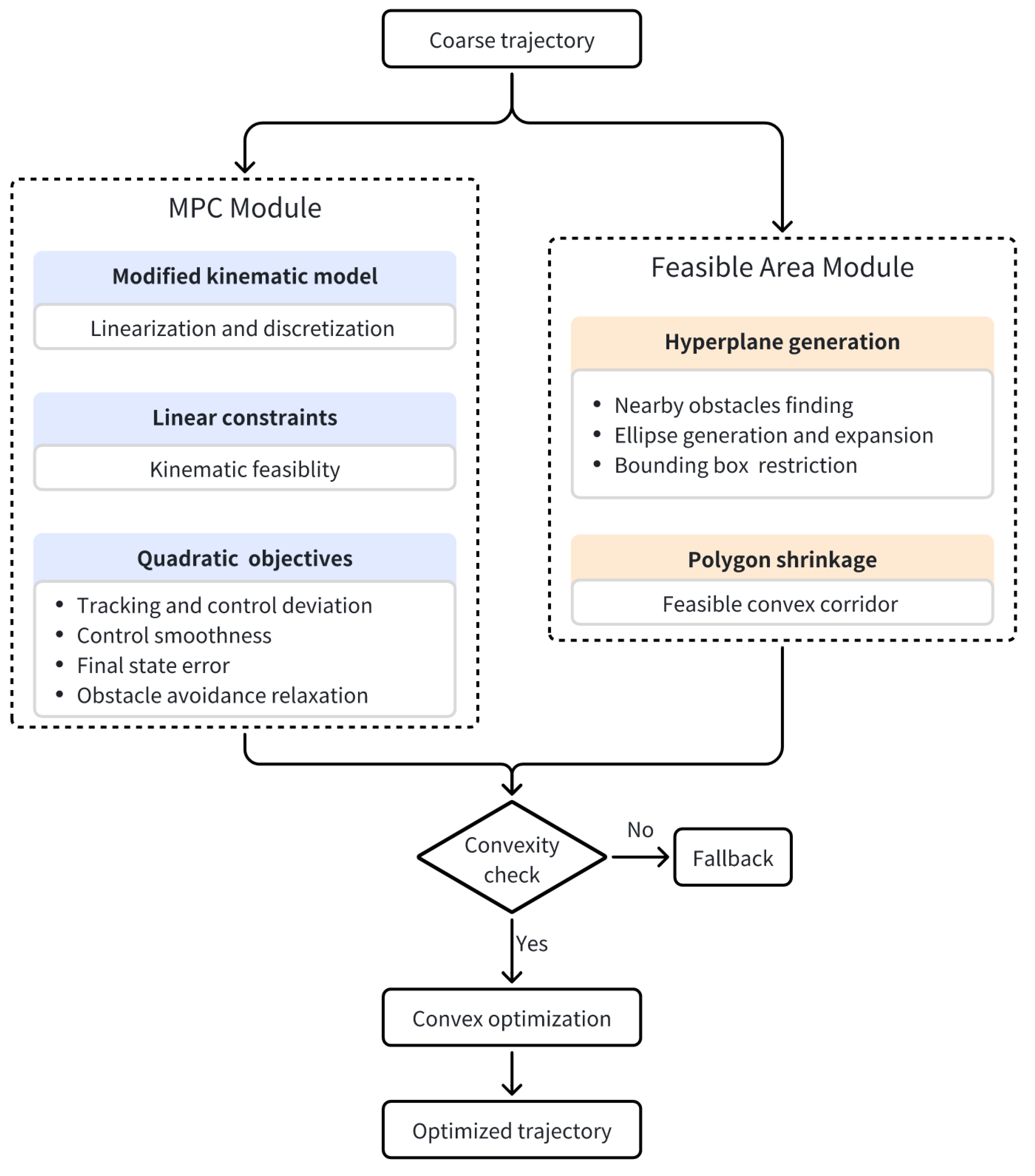
4. Proposed Optimization Method

This section outlines the proposed convex optimization-based trajectory planning framework. The general formulation is expressed as follows:

$$min{\displaystyle \frac{1}{2}}{x}^{T}Qx+c^{T}x,$$

$$s.t.A_{eq}x=b_{eq},$$

$$A_{ieq}x\le b_{ieq},$$

where $\mathbf{x}\in R^n$ denotes the vector of optimization variables, Q is the Hessian matrix containing second-order derivatives, and c is the gradient vector. Equality and inequality constraints are defined by matrices $A_{eq},A_{ieq}$ and vectors $b_{eq},b_{ieq}$, respectively. The framework comprises two key modules:

• A MPC module that incorporates the new kinematic model;
• A feasible area generation module to ensure environmental safety.

These modules jointly determine whether the convexity condition holds. If satisfied, the framework solves a quadratic program to generate a smooth and optimized trajectory. A schematic overview is shown in Figure 4.

4.1. MPC Algorithm

The MPC module predicts future system behavior over a finite horizon N, solving an optimization problem at each time step. Only the first control input is applied, and the process repeats with updated system states.

For the sake of simplicity, we assume that the states are always measurable and there is no model mismatch. The objective functions to be optimized can be stated as a quadratic function of the states and control inputs:

• The tracking error penalizes deviation from the reference trajectory:

  $$f_1=w_1\sum {(\mathbf{x}-{\mathbf{x}}_{ref})}^2.$$

  (19)
• Control deviation penalizes differences between actual and reference control inputs:

  $$f_2=w_2\sum {(\mathbf{u}-{\mathbf{u}}_{ref})}^2.$$

  (20)
• Control smoothness penalizes rapid changes in control inputs:

  $$f_3=w_3\sum {\dot{\mathbf{u}}}^2.$$

  (21)
• The final state error encourages convergence to a desired final state ${\mathbf{x}}_{ref}\left(N\right)$:

  $$f_4=w_4{(\mathbf{x}\left(N\right)-{\mathbf{x}}_{ref}\left(N\right))}^2.$$

  (22)
• Obstacle avoidance enforces spatial constraints using a slack variable:

  $$f_5=w_5\sum s_i^2,$$

  (23)

  where $s_i$ is the relaxation factor introduced to maintain feasibility. Its role is elaborated in the following subsection.

The total cost is expressed as follows:

$$J=\sum _{i=1}^5{w}_i{f}_i.$$

(24)

To ensure the kinematic feasibility of the vehicle, the following inequality constraints must be satisfied:

• Linear velocity: $v_{min}\le v\le v_{ma\mathbf{x}}$.
• Acceleration: $a_{min}\le a\le a_{ma\mathbf{x}}$.
• Jerk: ${\dot{a}}_{min}\le \dot{a}\le {\dot{a}}_{ma\mathbf{x}}$.
• Curvature: $k_{min}\le k\le k_{ma\mathbf{x}}$, $k={\displaystyle \frac{tan\left(\delta \right)}{L}}$.

4.2. Feasible Area Generation

To ensure the vehicle remains within a safe, obstacle-free region during planning, we construct a convex spatio-temporal corridor along a given reference trajectory. The position of dynamic obstacles is incorporated as a time-indexed sequence over the planning horizon, allowing the optimizer to account for predicted future motion patterns at each timestep. The method is structured into two main phases: hyperplane generation and polygon shrinkage.

4.2.1. Hyperplane Generation

We first approximate the vehicle’s rigid body using an ellipse. An ellipse is defined by the following:

$$\xi (E,d)=\{p=E\overline{p}+d,|\overline{p}|\le 1\},$$

(25)

where $E=R^{T}SR$, with R being the rotation matrix determined by the vehicle’s heading angle, and S a diagonal matrix with the ellipse’s semi-axes lengths. The vector d denotes the center of the ellipse. To fully enclose the vehicle, we compute the radius of a circle that covers its rigid body:

$$R=\sqrt{{\displaystyle \frac{{(L_r+L+L_f)}^2+L_w^2}{2}}},$$

(26)

where $L_r,L_f,L_w$ are the lengths of the rear axle, front axle, and vehicle width, respectively. The ellipse is scaled until it precisely wraps the vehicle. To maintain spatial continuity along the trajectory, we also consider the piecewise path segments when generating the ellipse. This guarantees that each segment of the trajectory remains constrained within a continuous, smooth corridor. We then expand the ellipse while preserving its aspect ratio until it touches an obstacle. At the contact point, a tangent hyperplane is computed:

$$H_i=\{\ell |a_i^T\ell <b_i\},$$

(27)

where $a_i\in {\mathbb{R}}^2$ and $b_i\in \mathbb{R}$ define the hyperplane, and $\ell =\{x,y\}$ is the vehicle position. Obstacles lying outside the hyperplane are disregarded. Repeating this process yields a series of half-spaces whose intersection forms a convex polygon:

$$S={\bigcap }_{i=0}^n{H}_i=\{\ell |A^T\ell <b\}.$$

(28)

Here, the i-th column of matrix A and element of vector b correspond to the coefficients of the i-th hyperplane. To reduce computational complexity and maintain proximity to the initial trajectory, a bounding box is introduced. This local region $R_{local}$ extends 10 meters laterally from the trajectory, while its longitudinal bounds are dynamically adjusted based on the vehicle’s speed. Then, the feasible area becomes $S=R_{local}\bigcap S$.

4.2.2. Polygon Shrinkage

To ensure the entire vehicle is fully contained within the convex polygon, it is necessary and sufficient that all vertices of the vehicle remain inside the polygon’s boundaries. To simplify computation, we convert this multi-vertex check into a point-based representation by applying a shrinkage process.

We first compute a new hyperplane $H_{i1}$ parallel to $H_i$, located at the distance from the vehicle’s rear axle:

$$H_{i1}=a_i^T\ell -b_{i1}.$$

(29)

We also define $H_{i2}$, where the vehicle’s vertex would collide with the original hyperplane:

$$H_{i2}=a_i^T\ell -b_{i2}.$$

(30)

The shrinkage criterion requires the contracted hyperplane $H_{i3}$ to be as equidistant to $H_{i1}$ and $H_i$ as $H_i$ is to $H_{i2}$. This indicates that once the rear axle of the vehicle reaches the hyperplane $H_{i3}$, the vehicle is at the collision threshold. This criterion ensures that the shrinkage accurately captures the vehicle’s potential collision risk, enabling precise adjustments to avoid obstacles while maintaining a safe and feasible trajectory. Thus, we have the following:

$$H_{i3}=a_i^T\ell -b_i-b_{i1}+b_{i2}.$$

(31)

Shrinkage may result in the exclusion of certain trajectory segments, potentially leading to discontinuities in the feasible region. To ensure the continuity of the trajectory, it is essential to verify that each segment of the piecewise path remains fully contained within the boundaries of the shrunken polygon. To accomplish this, we introduce a feasibility check step: for each half-space $H_{i3}$, we calculate the minimum distance from the trajectory segment to the hyperplane. The modified hyperplane $H_{i4}$ is represented as follows:

$$H_{i4}=a_i^T\ell -b_i-b_{i1}+b_{i2}-min(0,dist(\ell ,H_{i3}))=a_i^T\ell -b_i^c.$$

(32)

This guarantees continuous and feasible paths. The final convex constraint for obstacle avoidance is as follows:

$$S={\bigcap }_{i=0}^n{H}_{i4}=\{\ell |A^T\ell <b^c\}.$$

(33)

Additionally, we introduce a soft constraint to enhance obstacle avoidance. While the hard constraints ensure safety in scenarios where a collision is imminent, in practice, trajectory planning also seeks to maximize the distance from nearby obstacles whenever feasible. To achieve this, we introduce a safety margin parameter $s_i$ and shift the hyperplane accordingly. This results in a soft constraint that encourages the vehicle to maintain a safer buffer $b_i^s$ from obstacles:

$$H_{i5}=a_i^T\ell +s_i-b_i^s,b_i^s-b_i^c\le s_i\le 0.$$

(34)

The optimization variables are now extended as $x=[\overline{\mathbf{u}},\mathbf{s}]$, where

$$\overline{\mathbf{u}}=\left[\begin{array}{c}{\tilde{\mathbf{u}}}_0\\ {\tilde{\mathbf{u}}}_1\\ ⋮\\ {\tilde{\mathbf{u}}}_{N-1}\end{array}\right],\mathbf{s}=\left[\begin{array}{c}{s}_0\\ s_1\\ ⋮\\ s_n\end{array}\right].$$

With this, the convex optimization problem formulation is complete. The flow of the optimization framework is detailed in Algorithm 1. The proposed trajectory planning algorithm involves several sequential modules: geometric preprocessing (ellipse and corridor generation), linearized kinematic update, and final convex optimization via model predictive control (MPC). The detailed time complexity analysis is provided in

Table 2. Time-complexity analysis of the proposed algorithm.

Component	Description	Complexity
Ellipse generation	Geometric expansion until collision	$\mathcal{O}\left(O\right)$
Corridor shrinkage	Hyperplane refinement per waypoint	$\mathcal{O}\left(H\right)$
Waypoint iteration	Iterate over coarse trajectory of length T	$\mathcal{O}(T·(O+H\left)\right)$
Kinematic update	State propagation over horizon N	$\mathcal{O}\left(N\right)$
MPC optimization	QP solver with n variables, m constraints	$\mathcal{O}\left(n^p\right),p\in [1,3]$
Total	Overall end-to-end complexity	$\mathcal{O}(T(O+H)+N+n^p)$

.

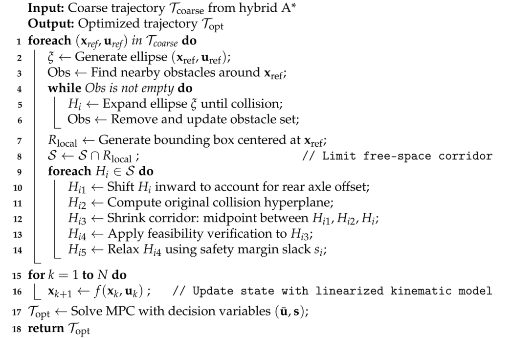
Algorithm 1: Convex optimization-based trajectory planning.

Let T denote the number of waypoints in the coarse trajectory. O the average number of nearby obstacles per point, and H the number of hyperplanes generated during corridor refinement. The MPC optimization horizon is N, and the final convex problem has n variables and m constraints. The total computational complexity of the algorithm is as follows:

$$\mathcal{O}\left(T·(O+H)+N+n^p\right),\mathrm{where}p\in [1,3],$$

where p depends on the choice of QP solver. This expression reflects the linear growth with trajectory length and obstacle density, and a convex QP solver-dependent cost for the MPC step. In practice, since N and n are moderate and modern solvers like OSQP exhibit near-linear performance, the entire algorithm remains suitable for real-time execution in urban driving scenarios.

5. Implementation and Experiments

In this section, we evaluate the effectiveness of the proposed convex optimization algorithm in terms of feasibility and trajectory quality.

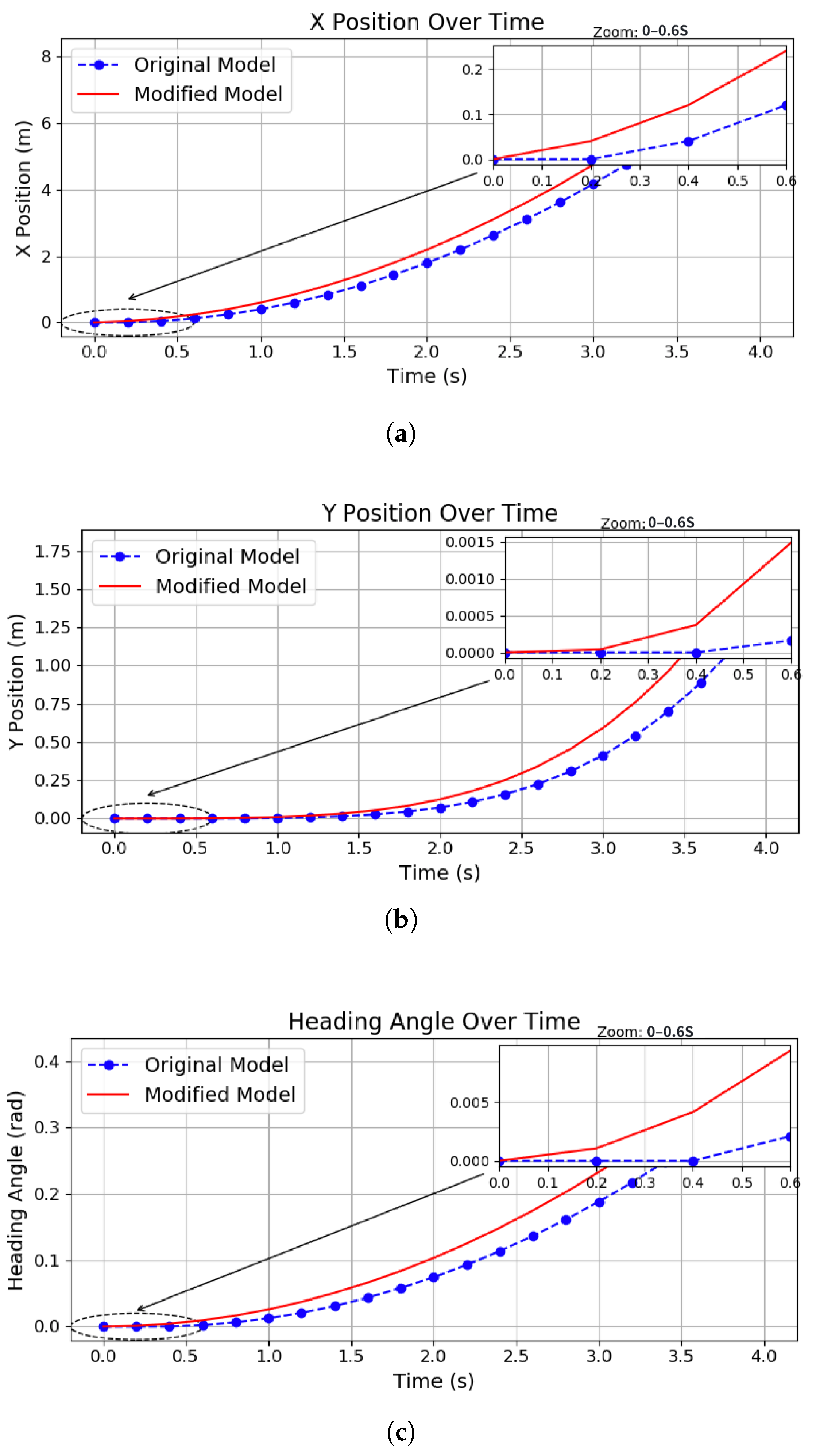
5.1. Kinematic Model Comparison

First, we compare two vehicle kinematic models (the original model Equation (1) that wildly used in previous works vs. the modified model Equation (8) that was proposed in our work) using identical initial conditions and control inputs. The scenario involved a vehicle starting from rest at the origin $(0,0)$, initially facing along the positive x-axis. A constant acceleration (a = 1 m/s²) and a fixed steering angle ($\delta$ = 0.15 rad) were applied over time. As shown in Figure 5, the original model (blue dashed line) shows no displacement in the X direction until around 0.4 seconds, maintaining a nearly constant position despite the presence of acceleration. In contrast, the modified model (red solid line) exhibits noticeable displacement starting as early as 0.2 seconds, indicating an earlier and more accurate response to the applied control input. This comparative simulation highlights critical differences between the original and modified kinematic vehicle models. The modified model more accurately captures the nuanced effects of acceleration and steering inputs on vehicle trajectories, position, and heading angle. Such detailed modeling is crucial for precise prediction and control applications in real-world applications. This behavior highlights the improved sensitivity and dynamic fidelity of the modified model, making it more suitable for real-time trajectory prediction in early motion stages.

To evaluate the computational efficiency of the proposed kinematic model, we conducted 100 repeated simulations for both the original and modified models under identical conditions. The execution time for each trajectory planning run was recorded. A boxplot (see Figure 6) visualizes the distribution of execution times for both models. The modified model achieves slightly lower average time with reduced variance, indicating better runtime stability. The statistical summary of execution time is presented in

Table 3. Statistical summary of execution time (in milliseconds).

Metric	Original Model	Modified Model
Minimum	0.07796	0.07820
Maximum	0.31710	0.32663
Mean	0.10150	0.09536
Median	0.08118	0.08082
Standard Deviation	0.03925	0.03038

. Our key observations are as follows:

• Similar overall distribution: Both models show tightly clustered execution times, mostly between 0.08 ms and 0.14 ms.
• Slightly higher stability in the modified model: While a few extreme outliers above 0.3 ms are observed in both cases, the modified model exhibits a narrower box and fewer outliers, suggesting more consistent performance.
• Real-time feasibility: Both models achieve average execution times well below 1 ms.

Despite incorporating more complex dynamics, the modified kinematic model does not introduce a noticeable increase in computational load. In fact, it demonstrates slightly better runtime stability while maintaining comparable average execution time. This supports its practicality for real-time trajectory optimization in urban autonomous driving scenarios.

5.2. Evaluation in Representative Driving Scenarios

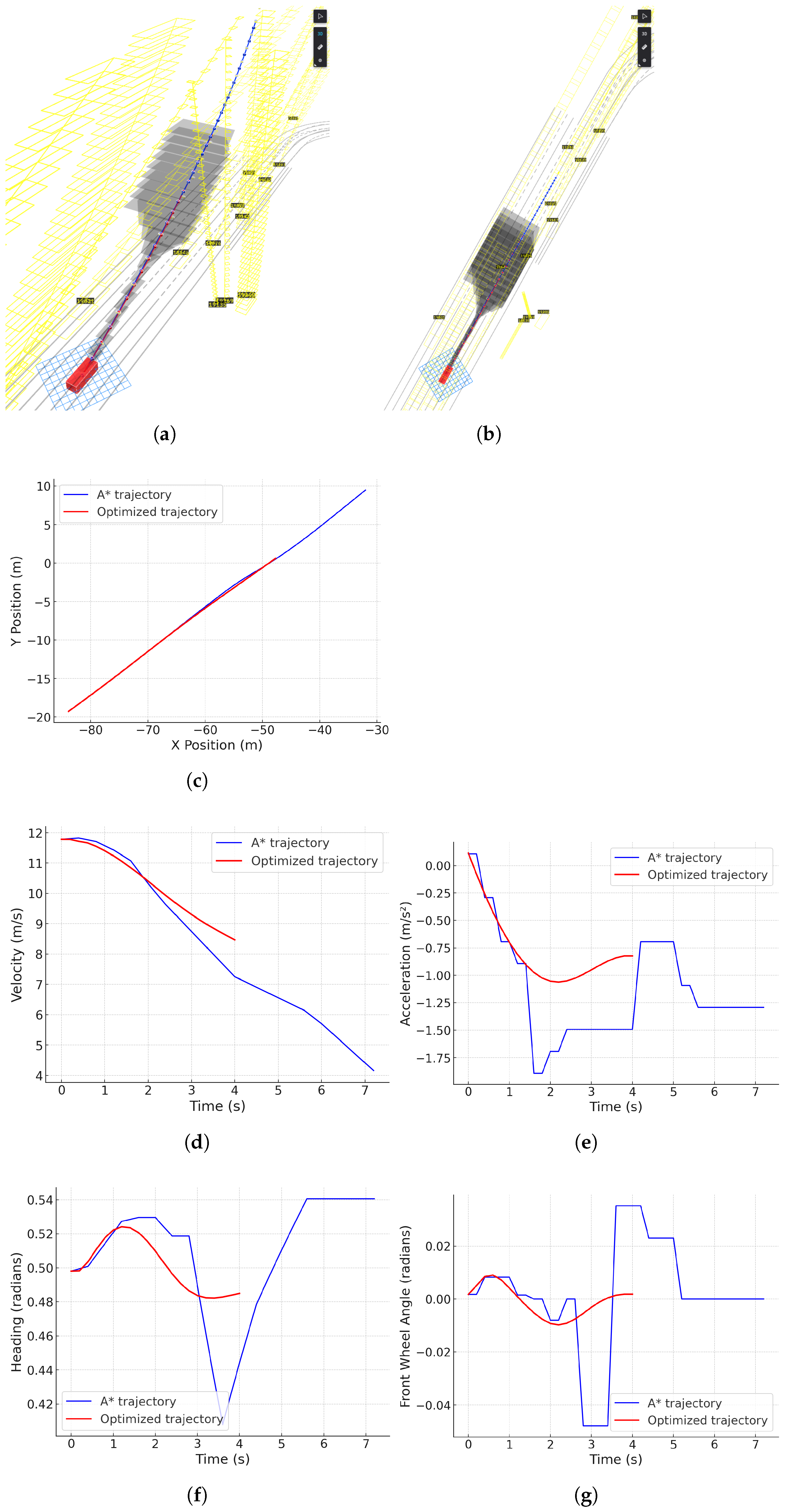
To demonstrate the performance of the proposed optimization method, two representative driving scenarios are considered: (1) the ego vehicle yielding to a cut-in vehicle, as shown in Figure 7, and (2) overtaking a slower vehicle, as shown in Figure 8.

The experiments are conducted in C++ on a laptop equipped with an Intel Core i7-12700 CPU. The OSQP solver is used to implement the optimization process. The planning horizon is 4 s. Initially, a coarse trajectory is generated using the hybrid A* algorithm. Subsequently, this initial guess was refined using the proposed convex optimization method, enhancing the trajectory’s smoothness, safety, and accuracy significantly. The optimization parameters are shown in

Table 4. Parameter configuration for trajectory optimization.

Symbol	Description	Value	Unit
$L_r$	Length of rear axle	0.615	m
$L_f$	Length of front axle	0.965	m
$L_w$	Vehicle width	1.800	m
L	Wheelbase	2.920	m
$v_n$	Navigation speed limit	derived from HD map	m/s
$\Delta t$	Time step	0.200	s
$v_{min}$	Lower bound of velocity	0	m/s
$v_{max}$	Upper bound of velocity	$v_n$	m/s
$a_{min}$	Lower bound of acceleration	−5.0	m/s2
$a_{max}$	Upper bound of acceleration	2.0	m/s2
${\dot{a}}_{min}$	Lower bound of jerk	−5.0	m/s3
${\dot{a}}_{max}$	Upper bound of jerk	5.0	m/s3
${\kappa }_{max}$	Max curvature	derived from velocity	m−1

.

5.2.1. Lane-Following Scenario

In the lane-following scenario illustrated in Figure 7, the ego vehicle demonstrates the ability to dynamically adjust its trajectory when another vehicle unexpectedly cuts in. The optimized trajectory exhibits smooth maneuvering, ensuring safety without sacrificing passenger comfort. Figure 7 clearly displays the vehicle trajectory, velocity profiles, acceleration patterns, heading angles, and front wheel angles, each indicating smooth and stable control behavior under dynamic constraints.

5.2.2. Lane-Changing Scenario

The lane-changing scenario (Figure 8) further validates the robustness of the proposed method in densely populated dynamic environments. This scenario simulates overtaking maneuvers where the ego vehicle needs to smoothly transition between lanes, maintaining optimal speeds and managing clearances from nearby vehicles. The detailed visualization of trajectory and associated vehicle dynamics such as speed, acceleration, heading, and steering angles confirms the effectiveness and reliability of the optimization-based planning method in realistic driving conditions.

To further evaluate passenger comfort and dynamic smoothness, we computed the jerk profiles for both lane-following and lane-changing scenarios. The resulting statistics are summarized in

Table 5. Jerk statistics for lane-changing and lane-following scenarios.

Scenario	Mean Jerk (m/s3)	Max Jerk (m/s3)	Min Jerk (m/s3)	Std Dev (m/s3)
Lane Changing	$-0.15$	$-0.02$	$-0.27$	$0.08$
Lane Following	$-0.23$	$0.21$	$-0.96$	$0.40$

. For the lane-changing case, the mean jerk was −0.15 m/s³ with a low standard deviation of 0.08 m/s³, indicating smooth transitions. For the lane-following case, a slightly higher mean jerk of −0.23 m/s³ and a standard deviation of 0.40 m/s³ were observed, reflecting stronger deceleration phases. In both cases, peak jerk values remain well within acceptable comfort thresholds for urban driving. These results confirm that the proposed optimization method produces not only dynamically feasible but also comfort-aware trajectories.

5.3. Computational Efficiency

The flame graph in Figure 9 illustrates the computational efficiency of the algorithm, showing the distribution of execution time among the different functions involved in trajectory optimization. In particular, the primary optimization function (planning::optimize::MPCOptimizer::OptimizeTrajectory) consumes only 0.88% of the total computational resources. This highlights the applicability of the proposed algorithm in real-time, which is essential for practical deployment in autonomous vehicles.

Figure 10 presents a comparative analysis of time consumption across iterations for two optimization strategies: nonlinear optimization [24] and proposed convex optimization. The x-axis denotes the planning iteration index, while the y-axis represents the time cost in milliseconds. Each data series is accompanied by a horizontal dashed line indicating its mean value.

The nonlinear optimization, plotted in blue, demonstrates relatively stable behavior across approximately 1800 iterations. The data are mostly concentrated between 30 and 36 ms, suggesting consistent performance but with a substantial computational cost. The average time cost is approximately 33.34 ms, as indicated by the blue dashed line. This high computational burden is attributed to the complexity of the nonlinear solver and the dimensionality of the optimization problem.

In contrast, the convex optimization process (shown in red) exhibits significantly lower time consumption, with an average of 9.47 ms per iteration. While the data show more pronounced variation than the nonlinear method, they remain bound within a practical range, typically oscillating between 8 and 12 ms. This result implies that the convex formulation offers a substantial improvement in computational efficiency, reducing average execution time by approximately 70% compared to the nonlinear alternative.

Despite the increased variance in the convex optimization time, the trade-off in favor of faster computation may make it more suitable for time-sensitive applications, such as real-time systems. Conversely, the nonlinear optimization may be preferable in offline computation.

5.4. Feasibility and Safety Analysis

Across a comprehensive set of tested scenarios, including varying curves, merging and diverging situations, and narrow roads, the proposed algorithm consistently generates feasible and safe trajectories. Convex polygons represent the feasible regions at each timestep, ensuring obstacle-free navigation through dynamic environments. The overlap between adjacent polygons guarantees continuity, allowing for seamless trajectory transitions over time. The experimental evaluations provided compelling evidence of the algorithm’s strengths:

• The spatial corridor generation framework significantly enhances safety, effectively addressing dynamic obstacle avoidance through both hard and soft constraints. This ensures vehicle trajectories maintain appropriate clearances from obstacles at all times.
• The formulation of convex optimization is vital for achieving efficient and reliable solutions. It not only guarantees global optimality but also supports real-time operations, critical for urban driving applications.

5.5. Discussion

The experimental results reinforce the effectiveness of the proposed algorithm in real-world scenarios, emphasizing its potential for practical deployment in autonomous driving systems. In future work, we aim to address several limitations and extend the proposed framework in multiple directions. First, to improve adaptability in inherently non-convex environments, SCP or iLQR will be considered. Additionally, we plan to incorporate dynamic obstacle interaction models—such as intention-aware predictors or game-theoretic frameworks—to better handle cooperative scenarios involving other vehicles or pedestrians. Furthermore, we intend to extend and incorporate estimation and uncertainty handling via risk-aware methods to account for sensor noise and partial observability. Finally, learning-based planning modules (e.g., L-MPC or imitation learning) and adaptive driving styles will be explored to improve generalization across diverse environments and user preferences.

6. Conclusions

Trajectory planning in autonomous driving faces inherent complexities due to non-convex obstacle avoidance regions, dynamic environmental constraints, and nonlinear objective functions. To effectively address these challenges, this paper has introduced a novel convex optimization framework tailored for trajectory planning in complex urban driving scenarios. By integrating a newly developed extended vehicle kinematic model, our approach accurately reflects dynamic vehicle behaviors, including effects of acceleration and steering inputs, improving trajectory prediction and responsiveness.

Another key innovation presented is the convexification of obstacle constraints using free-space corridor techniques, which simplifies the challenging non-convex optimization problem into a solvable convex form. Furthermore, embedding the planning method within a linearized model predictive control (MPC) framework ensures computational efficiency and facilitates real-time applicability crucial for urban driving environments. Experimental evaluations conducted in various driving scenarios, ranging from lane following with sudden vehicle interactions to complex lane changing, demonstrate the robustness and effectiveness of our proposed method. These experiments have illustrated improvements in trajectory smoothness, safety margins, and real-time computational performance. The method consistently produces collision-free and dynamically feasible trajectories while maintaining high computational efficiency, making it highly suitable for deployment in real-world autonomous driving systems.

Overall, the proposed convex optimization approach represents a balanced trade-off among computational efficiency, safety, trajectory smoothness, and dynamic adaptability. Future research directions include extending this method to consider environmental uncertainties, sensor data integration, and robustness against dynamic changes in traffic flow and road conditions, thus further enhancing its practical utility in more demanding real-world scenarios.