Improved Rectangular Extension of Steinmetz Equation Including Small and Large Excitation Signals with DC Bias

Abstract

The core loss of the ferrite-based magnetic components is usually characterized by the well-known Steinmetz equation and its derivatives. This occurs when the magnitude of the excitation signal is high enough; otherwise, the core loss is defined by the complex permeability. These two models are based on different assumptions, and thus, this paper aims to combine the large- and small-signal core loss models into a single, unified model. Moreover, the paper presents improvements to the existing state-of-the-art core loss model, specifically regarding the influence of the switching duty-cycle of rectangular excitation signals and the DC bias.

1. Introduction

The ferrite-based core loss characteristics provided by the core manufacturers are designed to calculate the average power loss per unit volume or mass. The characteristics are estimated by the well-known original Steinmetz equation (OSE) [1], which is

$$P_{OSE}=k{f}^{\alpha }{B}_m^{\beta }$$

(1)

where k, α, and β are the Steinmetz coefficients obtained during the fitting of the double logarithmic core loss characteristics given by the core manufacturers, f is the switching frequency, and B_m is the amplitude of the magnetic flux density.

Unfortunately, the equation, despite its simplicity, does not account for non-sinusoidal excitation signals, such as rectangular waveforms and their DC bias, a situation that often prevails in modern switch-mode power supplies (SMPS).

As shown in various works, the rectangular excitation waveforms have a profound impact on the core loss, especially at the minimum and maximum values of the switching duty-cycle. Therefore, to address this issue various core loss models dedicated to the non-sinusoidal excitations have been designed: the MSE [2], GSE [3], iGSE [4], WcSE [5], i²GSE [6], RESE [7], ISE [8], FGSE [9], and SSLE [10]. These models, e.g., assume that the core loss is proportional to the magnetic flux density rate of change (dB/dt) [2,3,4,6]; assume that the magnetic flux density is piece-wise-linear, allowing separate calculations of the power loss of each minor and major B–H loop [4,6]; and include the relaxation phenomenon during the zero-voltage transition periods [6,8,9] and/or DC bias [3,10]. These models attempt to predict the core loss accurately, but they often suffer from large numbers of hard-to-predict coefficients and overall method complexity.

Therefore, a new core loss model dedicated to the rectangular AC voltages, which is based on the rectangular extension of the Steinmetz equation (RESE) [7] and called here an improved RESE (iRESE), is proposed.

The RESE [7] method itself is similar to the waveform coefficient Steinmetz equation (WcSE) [5], introducing the proportionality coefficient between the square and the sinusoidal waveform core losses. The coefficient in the RESE method is directly related to the measured core loss and is obtained by the comparison of the triangular and the sinusoidal magnetic flux densities of the same peak-to-peak values, and the resulting ratio is referred to the equivalent resistor loss at the same excitation signals. The main drawback of this method is the requirement for a lookup table regarding the $\gamma$ fitting coefficient. Moreover, this method in the original form does not consider the DC bias premagnetization. It was later improved in [11] and by Sanusi et al. in [12] by adding to the original methodology a study on a DC bias in the linear region and further extended by Rasekh et al. in [13] by introducing an offline compensation of phase discrepancy using offline impedance sweep and the FFT analysis. Nevertheless, the method is considered to be more accurate than the MSE, GSE and the iGSE methods for rectangular excitation signals [2,3,4].

The iRESE unifies the Steinmetz-based core loss model with the small-signal complex permeability model to comprehensively complete the entire core loss characteristics regardless of the magnitude of the excitation signals.

The unification of both models seems to be imminent both (i) because that is how the inductor really behaves, and (ii) because the single model can be used in both small- and large-signal domains, which was not possible before.

Moreover, it also considers the rectangular excitation of signals and the DC bias phenomenon commonly present in the switch-mode power supplies (SMPS), altogether with the magnetic permeability roll-off near the core saturation level.

The model is also structured to be modular, meaning that each part of it can be used separately according to the intended application. This is a unique approach that provides engineers and scientists with all the required information at once regarding core loss, as well as the freedom of choice depending on the application they work on.

The method also discusses nonlinearity of the inductor magnetizing current and its impact on the core losses in small-signal domain, and thus, with an extra effort, the method can also be applied to the SPICE modelling and simulation, which is required by the industry for fast and precise estimation of the magnetic components’ core loss.

The proposed model has five degrees of freedom regarding the core loss in the ferrite materials and includes dependency on (i) the magnitude of the magnetic flux density, (ii) frequency of the excitation, (iii) temperature variations, (iv) the shape of the excitation signal, and (v) DC bias.

The method is applicable but not limited to the SMPS applications and can be also applied to any other arbitrary applications affected by the DC bias and rectangular excitation waveforms such as electric vehicle inverters and wireless power transfer systems.

2. Review of RESE Based Loss Models

The RESE model is specifically designed for rectangular AC voltage excitation. It is based on the ideal inductor model connected in parallel with the equivalent core loss resistor, as shown in Figure 1.

It introduces the proportionality coefficient to the OSE that is based on the measured data and serves as a link between the square and the sinusoidal excitation core losses. This coefficient is obtained by comparing the triangular and sinusoidal magnetic flux densities, both with the same peak-to-peak values, and the resulting ratio is referred to as the equivalent resistor loss at the same excitation signal. This gives a “U”-shaped core loss characteristic as a function of the duty-cycle ratio, a situation commonly encountered in switch-mode power supplies. An example of such characteristics is given in Figure 2.

The following equation expresses the method itself:

$$P_{RESE}={\displaystyle \frac{8}{{\pi }^2{\left[4D\left(1-D\right)\right]}^{\gamma +1}}}k{f}^{\alpha }{B}_m^{\beta }$$

(2)

where $D$ is the duty-cycle ratio; $k, \alpha , \beta$ are the Steinmetz coefficients; $\gamma$ is the material fitting coefficient.

The primary challenge seems to be the verification of the method, particularly due to the precise measurement of power loss versus duty-cycle ratio [7,11,12,13,14]. Typically, this is accomplished through voltage-current measurement using an oscilloscope, known as the two-windings method. This measurement approach, in its standard setup, measures the inductor magnetizing voltage across the inductor’s secondary windings and the magnetizing current across the current-sensing resistor placed on the primary side. This arrangement allows to avoid the influence of the inductor’s winding resistance and parasitics related to the leakage inductance. The core loss is then expressed by:

$$P_c={\displaystyle \frac{1}{R_{sense}}}\cdot {\displaystyle \frac{1}{T}}{\int }_0^T{v}_m{\left(t\right)v}_{Rsense}\left(t\right)dt$$

(3)

The equivalent circuit schematic and equivalent setup are given in Figure 3,

Figure 3. Standard two-winding measurement method; (a) conceptual diagram; (b) equivalent circuit schematic.

Figure 3. Standard two-winding measurement method; (a) conceptual diagram; (b) equivalent circuit schematic.

where $R_{cp}$—is the core parallel resistance.

The method can exclude the winding loss and applies to arbitrary excitation waveforms; however, it suffers from the sensitivity to phase discrepancy $\Delta {\varphi }_{sense}$, which is the phase angle difference between the measured voltage $v_{Rsense}$ across the sensing resistor and the magnetizing current $i_m$ flowing through it. This phase discrepancy leads to a core loss measurement error, especially profound at megahertz frequencies [11,14]. The error usually originates from the current sensing resistor’s parasitics, voltage probes’ frequency and amplitude discrepancies, and the oscilloscope’s resolution and sampling rate. Based on the study given in [15], the measurement error applicable to sinusoidal excitations can be expressed as:

$$\Delta =\tan \left({\varphi }_m\right)\cdot \Delta {\varphi }_{sense}$$

(4)

where ${\varphi }_m$ is the phase angle difference between the magnetizing voltage $v_m$ and the magnetizing current $i_m$. Typically, the magnetizing reactance of the tested transformer is significantly higher than the current sense resistor value, and therefore, the phase angle between the magnetizing voltage and the magnetizing current is close to $90°$. This leads to the situation where the $\mathrm{t}\mathrm{a}\mathrm{n}\left({\varphi }_m\right)$ in Equation (4) goes to infinity limit, significantly amplifying variations of phase discrepancy $\Delta {\varphi }_{sense}$, which causes an increase of the measurement error.

A similar relationship also applies to the rectangular excitation signals.

How severe the measurement error can be is illustrated in Figure 4 [11], where a $1°$ phase discrepancy can result in a 100% measurement error near a $90°$ phase angle.

The mitigation of the core loss measurement error in almost pure inductive environment was demonstrated in [11,16,17] by introducing the capacitive and inductive cancellation methods. As the capacitive cancellation is dedicated to the sinusoidal excitations only, and since this work is dedicated to the square excitation signals, the capacitive cancellation will be excluded from the discussion.

The inductive cancellation method applies to any arbitrary waveforms, and the general idea behind it is to introduce a second inductor into the two-winding measurement circuit, as shown in Figure 5.

The added inductor is placed in such a way that it acts with the inductor under test and the remaining components of the test-bench circuitry, canceling the reactive voltage [11,14,16,17]. This brings the $90°$ phase angle between the magnetizing voltage $v_m$ and the magnetizing current $i_m$ near to $0°$, revealing a purely resistive core loss.

In this case, the Equation (3) can be rewritten as:

$$P_c={\displaystyle \frac{1}{R_{sense}}}\cdot {\displaystyle \frac{1}{T}}{\int }_0^T{v}_{res}{\left(t\right)v}_{Rsense}\left(t\right) dt$$

(5)

where $v_{res}$ is the cancellation voltage across the inductive resonant tank.

The measurement error becomes then:

$$\Delta =\tan \left({\varphi }_{res}\right)\cdot \Delta {\varphi }_{sense}$$

(6)

where ${\varphi }_{res}$ is the phase angle between $v_{res}$ and $i_m$.

If the cancellation inductance $L$ is placed in series with $L_m$ the reactive voltage of the DUT is cancelled out, and the measurement error tends to zero.

In principle, this reactive power cancelation [11,14,16,17] scheme can be considered as comparing a reference air transformer core loss with the core loss under test. If the reactive power is cancelled during resonance, the power loss difference between the two is the core loss of the inductor under test.

Despite the method’s accuracy and its simplicity, it suffers from sensitivity to the cancellation inductance value. If the cancellation inductance does not perfectly match the inductance of the tested core, a significant jump in ${\varphi }_{res}$ occurs, leading to meaningful measurement errors, as shown in Figure 6 [14].

This makes the method impractical both industrially and technically, as inductance trimming might be very challenging and time-consuming. The relationships between the critical inductance $L_0$, the magnetizing inductance $L_m$ and the reference inductance $L$ to achieve perfect cancellations for sinusoidal excitation is given by [14]:

$$L_0=L_m\cdot {\displaystyle \frac{R_{cp}^2}{R_{cp}^2+{\left(\omega L\right)}^2}}$$

(7)

$${\mathsf{\varphi }}_{\mathrm{r}\mathrm{e}\mathrm{s}}=\arctan \left[\left(1-{\displaystyle \frac{\mathrm{L}}{{\mathrm{L}}_0}}\right)\cdot \mathrm{t}\mathrm{a}\mathrm{n}({\varphi }_m)\right]$$

(8)

Furthermore, Mu’s method suffers from one more disadvantage. Because the tested cores usually have high magnetic permeability, it is difficult to build a matching air or low core loss transformer. It requires a large number of turns, which introduces significant and undesired windings’ capacitance and other parasitic elements in the measurement. Therefore, the method is suitable only for low-inductance inductors.

The improvement to Mu’s cancellation method, known as the partial cancellation method, was introduced by Hou et al. in [14].

Hou’s method eases the constraints on matching the magnetizing inductance of the core under test with the critical inductance of the reference air transformer by introducing the cancellation factor $k$. The cancellation factor compensates for the mismatch between $L_m$ and $L$ as in Figure 5; therefore, an exact matching between $L_m$ and $L$ is not necessary. The conceptual circuit diagram for this method is given in Figure 7.

In this method, it is assumed that there are three sources of discrepancies during the core loss measurement: (i) $\Delta {\varphi }_{im}$ the phase discrepancy between the measured voltage across the sensing resistor $v_{Rsense}$ and the real magnetizing current flowing through it $i_m$, (ii) $\Delta {\varphi }_m$ the phase discrepancy between the measured ${v_m}^{\prime }$ and real $v_m$, and (iii) $\Delta {\varphi }_L$ the phase discrepancy between the measured ${v_L}^{\prime }$ and real $v_L$.

Considering the sinusoidal excitation, the cancellation of the $\Delta {\varphi }_{im}$ (if $\Delta {\varphi }_m=\Delta {\varphi }_L=0)$ can be done by the introduction of the cancellation factor $k$, which is:

$$k={\displaystyle \frac{V_L}{V_m\cdot sin{\varphi }_m}}$$

(9)

where ${\varphi }_m$ is the phase difference between the magnetizing current $i_m$ and the magnetizing voltage $v_m$.

Then the core loss can be calculated as follows:

$$P_c={\displaystyle \frac{1}{R_{sense}}}\cdot {\displaystyle \frac{1}{T}}{\int }_0^T{v}_m{v}_{Rsense}dt-{\displaystyle \frac{1}{k}}\cdot {\displaystyle \frac{1}{R_{sense}}}\cdot {\displaystyle \frac{1}{T}}{\int }_0^T{v}_L{v}_{Rsense}dt$$

(10)

Because the $V_m\cdot sin{\varphi }_m$ cannot be directly calculated, the phase disturbance needs to be introduced to the voltage across the sensing resistor, giving:

$$k={\displaystyle \frac{{\int }_0^T{v}_L{v^{\prime }}_{Rsense}dt-{\int }_0^T{v}_L{v}_{Rsense}dt}{{\int }_0^T{v}_m{v^{\prime }}_{Rsense}dt-{\int }_0^T{v}_m{v}_{Rsense}dt}}$$

(11)

The perturbation cannot be too big or too small, the suggested optimum is $\Delta {\varphi }_{im}^{\prime }=1°$.

The remaining phase discrepancies $\Delta {\varphi }_m$ and $\Delta {\varphi }_L$ can be calculated assuming that the $\Delta {\varphi }_{im}$ compensate during the calculation process [14]. In this case, it can be written:

$${\displaystyle \frac{1}{R_{sense}}}\cdot {\displaystyle \frac{1}{T}}{\int }_0^T{v}_m^{\prime }{v}_{Rsense}dt-{\displaystyle \frac{1}{k}}\cdot {\displaystyle \frac{1}{R_{sense}}}\cdot {\displaystyle \frac{1}{T}}{\int }_0^T{v^{\prime }}_L{v}_{Rsense}dt=P_c+V_m\cdot sin{\varphi }_m\cdot I_m\cdot \left(\Delta {\varphi }_m-\Delta {\varphi }_L\right)$$

(12)

where ${v^{\prime }}_m$ and $v_L^{\prime }$ are the measured voltages.

There exists a measurement error due to the remaining phase discrepancy $\Delta {\varphi }_m-\Delta {\varphi }_L$. It is caused by the phase mismatch between two voltage probes measuring $v_m$ and $v_L$. This can be eliminated by measuring the same voltage by both of the probes and then calculating an integral $\frac{1}{R_{sense}}\cdot \frac{1}{T}{\int }_0^T{v}_m^{\prime }{v}_{Rsense}dt$ for each of them. The results should be adjusted by a deskew function in the oscilloscope until the calculated integrals show the same value.

Considering the rectangular excitation waveforms, the cancellation factor is given by [11,14]:

$$k={\displaystyle \frac{V_{L(pk-pk)}}{V_{m(pk-pk)}}}$$

(13)

where $V_{L(pk-pk)}$ and $V_{m(pk-pk)}$ are the peak-to-peak values of $V_L$ and $V_m$, respectively.

The work of Mu [11,17] and Hou [14] was further extended by Sanusi et al. in [12] by adding to the original methodology a study on DC bias magnetization in linear region and also by Rasekh et al. in [13] by introducing an offline compensation of phase discrepancy using offline impedance sweep and the FFT analysis.

The area for improvement in Hou’s models is to extend core loss calculations into the near-saturation non-linear region and also add the losses existing in small-signal domain by combining the complex permeability small-signal model with the large-signal Steinmetz based model. This results into one unified and comprehensive core loss model in all signal domains.

3. Review of Small- and Large-Signal Core Resistance Calculation Methodologies

There are two concurrent core resistance calculation methodologies: (i) the small-signal core resistance calculation method, which is based on the complex permeability values, and (ii) the large signal core resistance calculation method based on the Steinmetz equation, which depends on the magnitude of the excitation signal.

3.1. Small-Signal Core Resistance

The small-signal core resistance of an inductor is given by [18,19]:

$$R_c=Re\left(j\omega \cdot {\displaystyle \frac{N^2}{\frac{l_C}{A_c{\mu }_r^{*}{\mu }_0}+R_g}}\right)$$

(14)

where $R_c$ is the series core resistance, $A_c$ is the effective cross-section of a magnetic core, $N$ is the number of winding turns, $l_c$ is the effective magnetic length of the core, ${\mu }_0$ is the magnetic permeability of the free air, $\omega$ is the angular frequency, $R_g$ is the air gap reluctance,${\mu }_r^{\ast }={\mu }_r^{\prime }-j{\mu }_r^{″}$ is the complex magnetic permeability.

Regarding the gapless inductor, Equation (14) becomes:

$$R_c={\displaystyle \frac{{\mu }_r^{″}{\mu }_0{N}^2{A}_c\omega }{l_c}}$$

(15)

where ${\mu }_r″$ is the imaginary part of the complex permeability.

According to the IEC 62044−2 [20], the small-signal imaginary part of the complex permeability of an inductor under test can be calculated as follows:

$${\mu ″}_r={\displaystyle \frac{l_c}{{\mu }_0{A}_c{N}^2}}\cdot {\displaystyle \frac{r}{\omega }}$$

(16)

where $r$ is the real part of impedance measurement, and the measurement should be done at a testing signal not exceeding $B_m=0.25 \left[mT\right]$.

However, as shown in Figure 8, an inductor is a complex system [18,19,21]; therefore, the real part of the impedance measurement is, in fact, a combination of many variables coming from the inductor’s parasitics.

The relation expressing this variables’ mix is given by:

$$r={\displaystyle \frac{{\omega }^4{L}_s^2{C}_s^2{R}_{Cs}+{\omega }^2{C}_s^2{R}_{cw}{R}_{Cs}\left(R_{cw}+R_{Cs}\right)+R_{cw}}{{\left(1-{\omega }^2{L}_s{C}_s\right)}^2+{\left(\omega C_s\left(R_{cw}+R_{Cs}\right)\right)}^2 }}$$

(17)

where $C_s$—inductor stray capacitance measured at self-resonance, $R_{c_s}$—inductor stray capacitance equivalent series resistance, $L_s$—inductor series inductance measured at low frequencies, $R_c$—equivalent core series resistance, $R_w$—windings resistance, $R_{cw}=R_w+R_c$—core and windings equivalent series resistance.

Thus, the best way to extract the core resistance from this complex equation is to use an iterative approximation curve fitting as shown in [21], which takes into account all the variables seen in Figure 8.

Another approach to calculating the core resistance is to measure the core parallel resistance $R_{cp}$ of an inductor at a self-resonant frequency and then transfer it to the series one as follows [18,19]:

$$R_c={\displaystyle \frac{{\left(\omega L\right)}^2{R}_{cp}}{{\left(\omega L\right)}^2+R_{cp}}}$$

(18)

The inductor core parallel resistance $R_{ cp}$ is constant and well-defined at inductor self-resonance; however, the inductance $L$, seen by the impedance analyzer changes along the frequency range, depends on the magnitude of the testing signal and is also a complex function of the inductor reactance and its parasitic variables, which is [19,21]:

$$x={\displaystyle \frac{{\omega }^3{L}_s{C}_s(C_s{R}_{Cs}^2-L_s)-\omega C_s{R}_{cw}^2+\omega L_s }{{\left(1-{\omega }^2{L}_s{C}_s\right)}^2+{\left(\omega C_s\left(R_{cw}+R_{Cs}\right)\right)}^2}}$$

(19)

Therefore, the approach using Equation (18) must also be carefully examined, as many factors influence the result, and an iterative approximation may also be involved in the calculations.

The fastest and probably one of the most accurate methods for calculating core resistance is to use an advanced impedance analyzer, such as the Agilent/HP 4294A. The measurement, in this case, was performed using a standard two-winding, four-terminal method, as shown in Figure 3 and Figure 9 [18], respectively.

This type of impedance analyzer manages to precisely measure the impedance, even when testing high-Q materials, and where the phase difference between the magnetizing current and the magnetizing voltage is very close to 90°, as discussed in Section 2.

3.2. Large-Signal Core Resistance

In general form, the ohmic power loss can be expressed as:

$$P=I_{rms}^{2}R$$

(20)

where $I_{rms}$ is the RMS value of the current and $R$ is the resistance.

Regarding the core loss, Equation (20) can be reformulated into:

$$P_c={\displaystyle \frac{{\widehat{I}}_m^2{R}_c}{2}}$$

(21)

where ${\widehat{I}}_m$ is an amplitude of core magnetizing current and $R_c$ is the core series resistance.

On the other hand, the core power loss can be expressed using Equation (1), yielding:

$$P_c=V_{e}k{f}^{\alpha }{B}_m^{\beta }$$

(22)

where $V_e$ is the effective volume of the core.

Thus, the core resistance is given by:

$$R_c=2V_{e}k{f}^{\alpha }{B}_m^{\beta }{\widehat{I}}_m^{-2}$$

(23)

and adding temperature adjustment, it becomes:

$$R_c=2V_{e}k{f}^{\alpha }{B}_m^{\beta }{\widehat{I}}_m^{-2}({\xi }_1{T}^2-{\xi }_{2}T+{\xi }_3)$$

(24)

where $T$ is the temperature, ${\xi }_1, {\xi }_2, {\xi }_3$ are the temperature fitting coefficients.

As shown in Figure 10, the small- and large-signal core loss models exhibit completely different characteristics, which are not complementary and intersect each other.

Therefore, an educated choice is to find a characteristic that reflects a real behavior of the core loss regardless the magnitude of the excitation signal, as will be shown in the next section of this work.

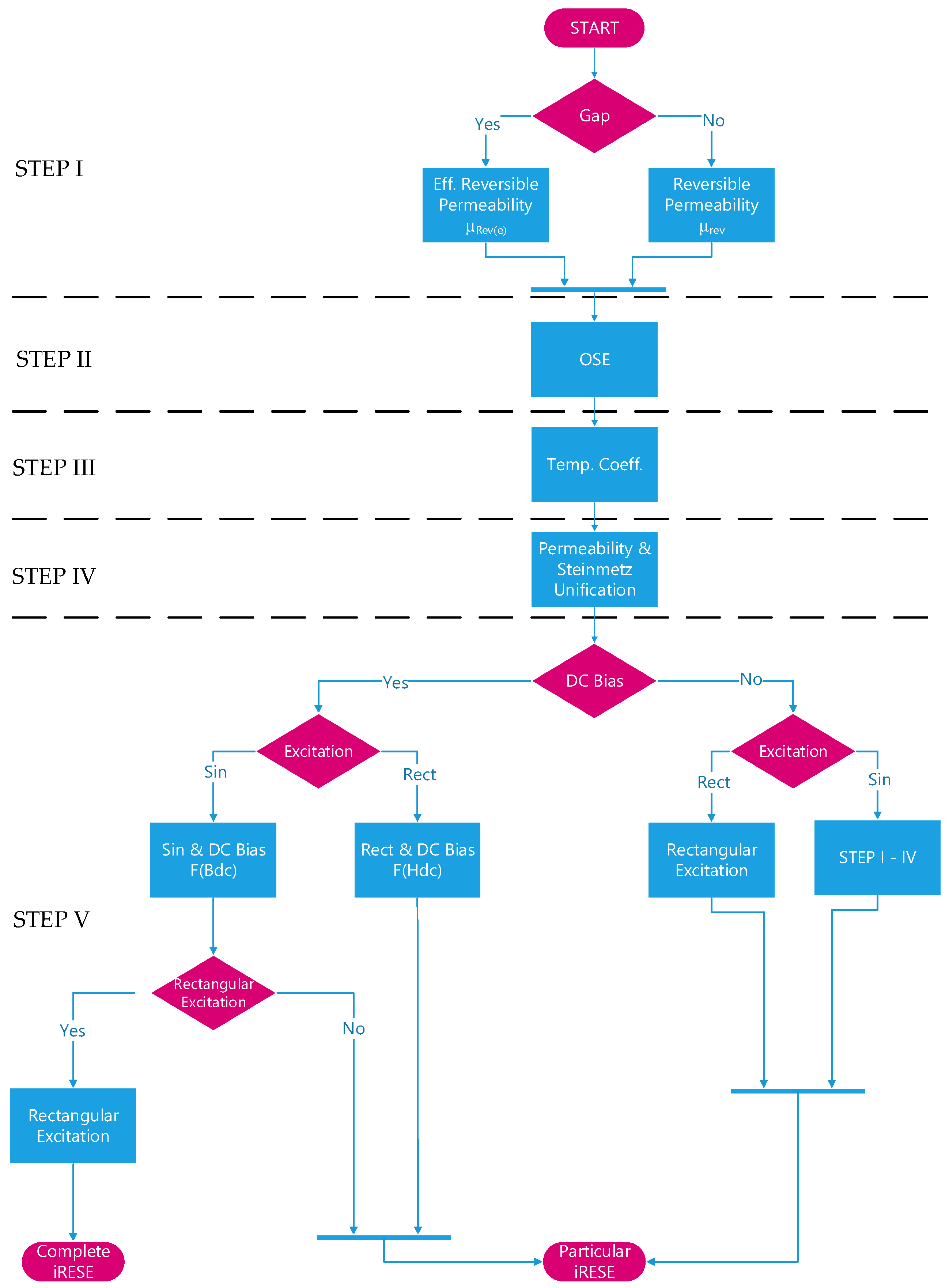
4. Proposed Core Loss Calculation Methodology

The proposed core loss calculation methodology is not intended to alter or dispute the core loss measurement approach proposed by Mu et al. [7,11,16,17] and Hou et al. [14]. It is simply because their methodologies have already been proven to be feasible and accurate [12,13], and Hou’s measurement method was used in this work to calculate the core loss. However, the new method, called here the improved RESE (iRESE), is rather an extension of the RESE model, pushing it into small- and near-saturation large-signal domains for both: sinusoidal and non-sinusoidal excitation signals, including a DC bias magnetization.

The knowledge about the core loss and the complex permeability in the small-signal domain can be used, e.g., in the design of the low-noise magnetic shielding [22], while the near-saturation operation is often used in SMPS as a trade-off between magnetic component efficiency, cost and size [23], or it can also be used for an application specific solution such as inrush current limiters [24].

The proposed methodology is assumed to be modular, meaning that its modules or steps can be used independently whenever the application involves sinusoidal or rectangular excitation signals.

The iRESE modular flowchart is given in Figure 11. It is divided into five significant steps to be presented subsequently.

STEP I:

The DC bias of the applied excitation signal levels off at the operating point, where the induction signal swings between its maximum and minimum values. If one of these extremes lies beyond the linear region of the B–H characteristics, then the magnetic permeability roll-off occurs. The same situation happens if the magnitude of the excitation signal without a DC bias is high enough to exceed the B–H linear region. This phenomenon affects the swing magnitude of the magnetic flux density at given field intensity values, pre-magnetizes the core, and thus increases the core loss.

The reversible permeability for sinusoidal excitations can be calculated using a method introduced by Esguerra et al. in [25,26,27,28,29]. The method is based on the Coleman–Hodgdon hysteresis model [30,31,32], which is given by:

$${\displaystyle \frac{dH}{dB}}=\pm \alpha \left({\displaystyle \frac{dB}{dt}}\right)\left(f\left(B\right)-H\right)+g(B)$$

(25)

where $f\left(B\right)$ and $g\left(B\right)$ are the material functions, $f\left(B\right)$ is the anhysteretic curve describing the hysteresis, $g\left(B\right)$ is the reversible function describing the drift from the anhysteretic curve, and $\alpha$ is the fitting parameter.

The method assumes that there is no need to define arbitrary $f\left(B\right)$ and $g\left(B\right)$ functions, but instead, an accurately measured major hysteresis loop can be used as a solution to Equation (25) and the minor hysteresis loops.

The empirical fit functions, which describe the lower and upper branches of the major hysteresis loop are given by:

$$H_L(B)={\displaystyle \frac{B}{{\mu }_0{\mu }_c}}\cdot {\displaystyle \frac{1}{1-{\left(\frac{B}{B_{sat}}\right)}^a}}+H_c$$

(26)

$$H_U\left(B\right)={\displaystyle \frac{B}{{\mu }_0{\mu }_c}}\cdot {\displaystyle \frac{1}{1-{\left(\frac{B}{B_{sat}}\right)}^b}}-H_c$$

(27)

where $H_L$ is the lower branch of the B–H curve, $H_U$ is the upper branch of the B–H curve, $B_{sat}$ is the assumed saturation of the magnetic flux density, $H_c$ is the coercive magnetic field intensity, $a, b$ are the fitting coefficients, $a\approx b$, ${\mu }_c$ is the magnetic permeability near the coercive magnetic field intensity, ${\mu }_0$ is the magnetic permeability of the free space.

Then the anhysteretic curve can be described as:

$$H\left(B\right)=H_L\left(B\right)-H_c{\left(1-{\displaystyle \frac{B}{B_{sat}}}\right)}^{\tau }$$

(28)

$$\tau ={\alpha }_0{B}_{sat}$$

(29)

$${\alpha }_0={\displaystyle \frac{1}{{\mu }_0{H}_c}}\left({\displaystyle \frac{1}{{\mu }_i}}-{\displaystyle \frac{1}{{\mu }_c}}\right)$$

(30)

where ${\mu }_i$ is the initial magnetic permeability.

The reversible permeability for an ungapped core can be calculated as follows:

$${\mu }_{rev}={\displaystyle \frac{1}{{\mu }_0}}\cdot {\displaystyle \frac{dB}{dH}}={\displaystyle \frac{1}{{\mu }_0}}\cdot {\left({\displaystyle \frac{dH}{dB}}\right)}^{-1}$$

(31)

Using Equations (26)–(30) and substituting them into Equation (31) gives:

$${\mu }_{rev}={\left({\displaystyle \frac{1+\left(a-1\right){\left(\frac{B}{B_{sat}}\right)}^a}{{\left[1-{\left(\frac{B}{B_{sat}}\right)}^a\right]}^2}}{\displaystyle \frac{1}{{\mu }_c}}+{\displaystyle \frac{1}{\left(1-\frac{B}{B_{sat}}\right){\left(1-\frac{B}{B_{sat}}\right)}^{-{\alpha }_0{B}_{sat}}}}\left({\displaystyle \frac{1}{{\mu }_i}}-{\displaystyle \frac{1}{{\mu }_c}}\right)\right)}^{-1}$$

(32)

and with some empirical modifications, the Equation (32) becomes:

$${\mu }_{rev}={\left({\displaystyle \frac{1+\left(a-1\right){\left(\frac{B}{B_{sat}}\right)}^a}{{\left[1-{\left(\frac{B}{B_{sat}}\right)}^a\right]}^2}}{\displaystyle \frac{1}{{\mu }_c}}+{\displaystyle \frac{1}{\left(1-\frac{B}{B_{sat}}\right)\left[2-{\left(1-\frac{B}{B_{sat}}\right)}^{-{\alpha }_0{B}_{sat}}\right]}}\left({\displaystyle \frac{1}{{\mu }_i}}-{\displaystyle \frac{1}{{\mu }_c}}\right)\right)}^{-1}$$

(33)

The magnetic flux density values at a given magnetic field intensity regarding a DC bias give an anhysteretic magnetization curve described by:

$$H_{dc}={\displaystyle \frac{1}{{\mu }_0{\mu }_c}}\cdot {\displaystyle \frac{B_{dc}}{1-{\left(\frac{B_{dc}}{B_{sat}}\right)}^a}}$$

(34)

Considering the gapped inductor, the effective reversible permeability can be expressed as follows:

$${\mu }_{rev\left(e\right)}={\displaystyle \frac{{\mu }_{rev}}{1+\frac{{\mu }_{rev}\cdot l_g}{l_c}}}={\displaystyle \frac{1}{\frac{1}{{\mu }_{rev}}+\frac{l_g}{l_c}}}$$

(35)

where $l_g$ is the length of the air gap.

The effective magnetic field intensity at any ${\mu }_{rev\left(e\right)}$ is given by:

$$H_{dc\left(e\right)}=H_{dc}+{\displaystyle \frac{1}{{\mu }_{rev\left(e\right)}{\mu }_0}}\cdot B_{dc\left(e\right)}$$

(36)

The above considerations regard the sinusoidal excitations. Unfortunately, the reversible permeability and the B–H characteristics are not well-defined by any models [30] for rectangular excitation signals when saturation occurs. Therefore, in this case, the permeability roll-off must be calculated iteratively step-by-step at any given operating point. It also refers to the DC bias operating point. Empirically, the proposed method follows the lower B–H branch if the DC bias is positive.

As it was described in Section 2 (Equation (10)), Hou’s method [14] cancels the reactive power by comparing a reference air transformer core loss with the core loss under test. However, this is only valid in the linear region of the B–H characteristics. If saturation happens, e.g., in the case of a DC bias, the relationships $\frac{1}{R_{sense}}\cdot \frac{1}{T}{\int }_0^T{v}_m{v}_{Rsense}dt$ and $\frac{1}{k}\cdot \frac{1}{R_{sense}}\cdot \frac{1}{T}{\int }_0^T{v}_L{v}_{Rsense}dt$ do not change proportionally, introducing an error in the reactive power cancellation. This is because the voltage $v_L$ depends on linear coreless inductance and its permeability, while the voltage $v_m$ drops non-linearly as the magnetic permeability rolls off. Therefore, an additional proportionality factor, which compensates for this phenomenon, must be introduced into Equation (10), yielding:

$$P_c={\displaystyle \frac{1}{R_{sense}}}\cdot {\displaystyle \frac{1}{T}}{\int }_0^T{v}_m{v}_{Rsense}dt-{\displaystyle \frac{1}{\sigma }}\cdot {\displaystyle \frac{1}{\eta }}\cdot {\displaystyle \frac{1}{k}}\cdot {\displaystyle \frac{1}{R_{sense}}}\cdot {\displaystyle \frac{1}{T}}{\int }_0^T{v}_L{v}_{Rsense}dt$$

(37)

where $\sigma =\frac{{\mu }_{rev}}{{\mu }_r}$ is the proportionality factor taking into account small-signal magnetic permeability roll-off near saturation due to DC bias, ${\mu }_{rev}$ is the small-signal reversible permeability value, ${\mu }_r$ is the initial small-signal permeability value measured in the linear region, $\eta =\frac{{\mu }_{rev\left(a\right)}}{{\mu }_{r\left(a\right)}}$ is the proportionality factor taking into account large-signal magnetic permeability roll-off near saturation, ${\mu }_{rev\left(a\right)}$ is the large-signal reversible permeability value, and ${\mu }_{r\left(a\right)}$ is the initial large-signal permeability value measured in the linear region near $H_c$.

STEP II–IV:

As stated in [33], the core manufacturers’ data, as found in the cores’ datasheets, are subject to significant uncertainties. Therefore, the second step in the proposed methodology is to verify the original Steinmetz equation coefficients using the measuring method given by Hou et al. [14] under sinusoidal excitations.

This should give the following relationship:

$$P_c=V_{e}k{f}^{\alpha }{B}_m^{\beta }({\xi }_1{T}^2-{\xi }_{2}T+{\xi }_3)$$

(38)

However, as it will be shown in the test-bench verification section this relationship would be better fitted with the fifth-degree polynomial regarding core loss temperature dependency, yielding:

$$P_c=V_{e}k{f}^{\alpha }{B}_m^{\beta }\cdot \left(\sum _{n=0}^5{\xi }_n{T}^n\right)$$

(39)

As it was shown in Figure 10, the transition point between small and large excitation signals causes the Steinmetz characteristics to be horizontal. Because of the complexity, this non-linear behavior can be fitted by adding to the Equation (39) a ninth-degree polynomial, giving:

$$P_c=V_{e}k{f}^{\alpha }\left(B_m^{\beta }+\sum _{i=0}^9{\chi }_i{B}_m^i\right)\cdot \left(\sum _{n=0}^5{\xi }_n{T}^n\right)$$

(40)

where ${\chi }_i$ are the fitting coefficients of ninth-degree polynomial regarding magnetic flux density, and ${\xi }_n$ are the fitting coefficients of the fifth-degree polynomial regarding temperature dependency.

STEP V:

According to Figure 11 there are a few scenarios regarding this step, namely:

1.

If there is a sinusoidal excitation and a DC bias, then the Equation (40) becomes:

$$P_c=V_{e}k{f}^{\alpha }\left(B_m^{\beta }+\sum _{i=0}^9{\chi }_i{B}_m^i\right)\cdot \left(\sum _{n=0}^5{\xi }_n{T}^n\right)\cdot F(B_{dc})$$

(41)

where $F\left(B_{dc}\right)=\sum _{j=0}^4{\zeta }_j{B}_{dc}^j$ is the sinusoidal excitation and a DC bias magnetization function obtained with the help of Equations (25)–(36), and ${\zeta }_j$ are the fitting coefficients. This equation is purely dedicated to sinusoidal excitations with a DC bias.

2.

If the rectangular excitation takes place, the corresponding relationship can be added to Equation (41), giving:

$$P_c=V_e{\displaystyle \frac{8}{{\pi }^2{\left(4D\left(1-D\right)\right)}^{\gamma }}}\cdot k_1{f}^{\alpha }\left(B_m^{\beta }+\sum _{i=0}^9{\chi }_i{B}_m^i\right)\cdot \left(\sum _{n=0}^5{\xi }_n{T}^n\right)\cdot F(B_{dc})$$

(42)

where $k_1=\delta k, \delta , \gamma$ are the function fitting coefficients at $B_{dc}=0$.

The Equation (42) can be used to calculate the core loss at rectangular excitation signals if the DC bias and the characteristics from STEP V.1 are known. This equation represents the complete iRESE model.

3.

If there is a rectangular excitation without a DC bias, the Equation (40) changes as follows:

$$P_c=V_e{\displaystyle \frac{8}{{\pi }^2{\left(4D\left(1-D\right)\right)}^{{\gamma }_1}}}\cdot k_2{f}^{\alpha }\left(B_m^{\beta }+\sum _{i=0}^9{\chi }_i{B}_m^i\right)\cdot \left(\sum _{n=0}^5{\xi }_n{T}^n\right)$$

(43)

where $k_2={\delta }_{1}k, {\delta }_1, {\gamma }_1$ are the function fitting coefficients.

4.

If rectangular excitation comes together with a DC bias, the DC bias is added to rectangular core loss with the assumption that the duty ratio of the signals’ equals $D=0.5$. Because a complex relationship exists between B and H near the core saturation region the DC magnetization function to be added is rather a function of $H_{dc}$ than $B_{dc}$ as in Equations (41)–(42), yielding:

$$P_c=V_e{\displaystyle \frac{8}{{\pi }^2{\left(4D\left(1-D\right)\right)}^{{\gamma }_1}}}\cdot k_2{f}^{\alpha }\left(B_m^{\beta }+\sum _{i=0}^9{\chi }_i{B}_m^i\right)\cdot \left(\sum _{n=0}^5{\xi }_n{T}^n\right)\cdot F\left(H_{dc}\right)$$

(44)

where $F\left(H_{dc}\right)=\sum _{j=0}^4{ϵ}_j{H}_{dc}^j$ is the DC bias magnetization function, ${ϵ}_j$ are the fitting coefficients.

As is evident, the proposed iRESE method comprehensively and, on a modular basis, deals with the sinusoidal and rectangular excitation signals, with or without a DC bias. In the next section, the assumptions given above will be evaluated through test-bench measurements.

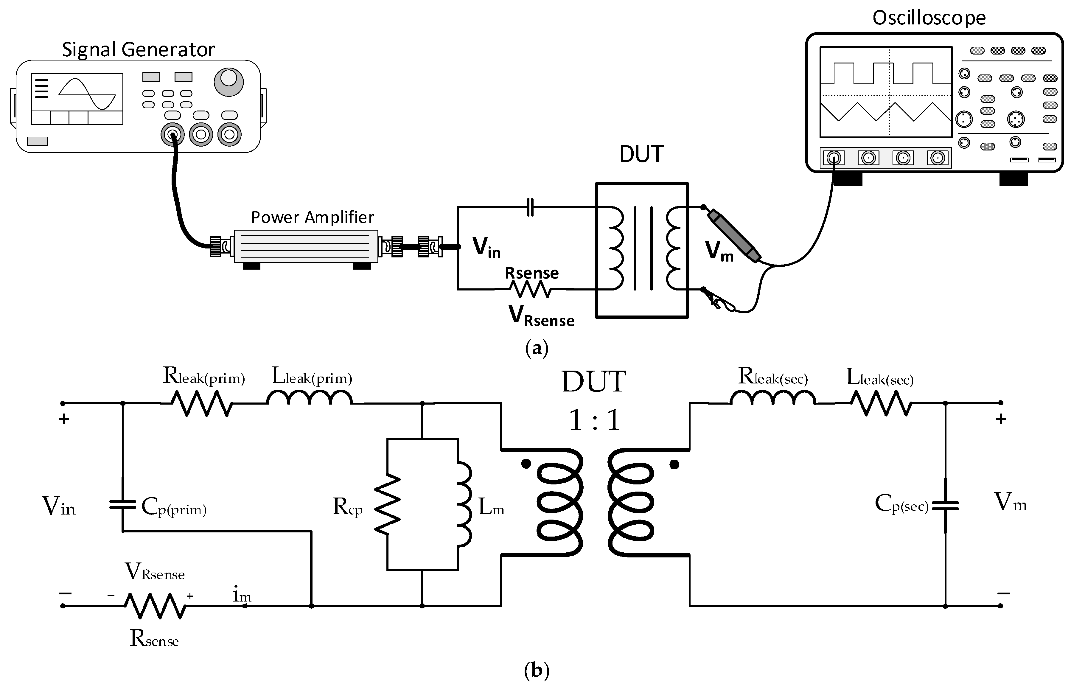
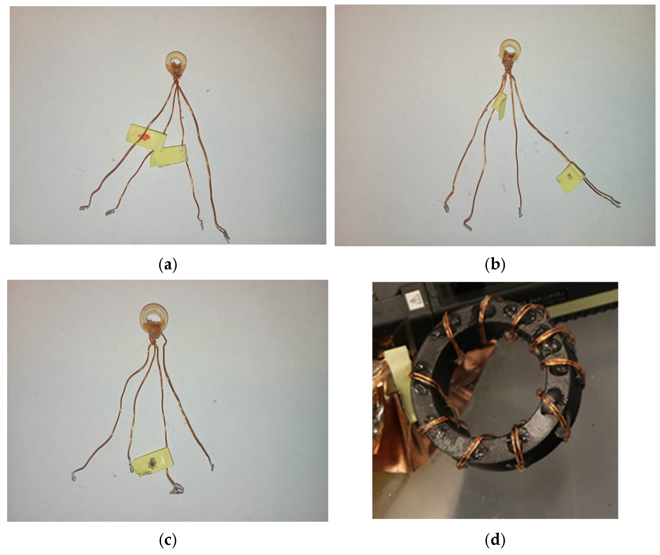
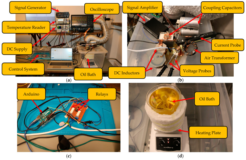
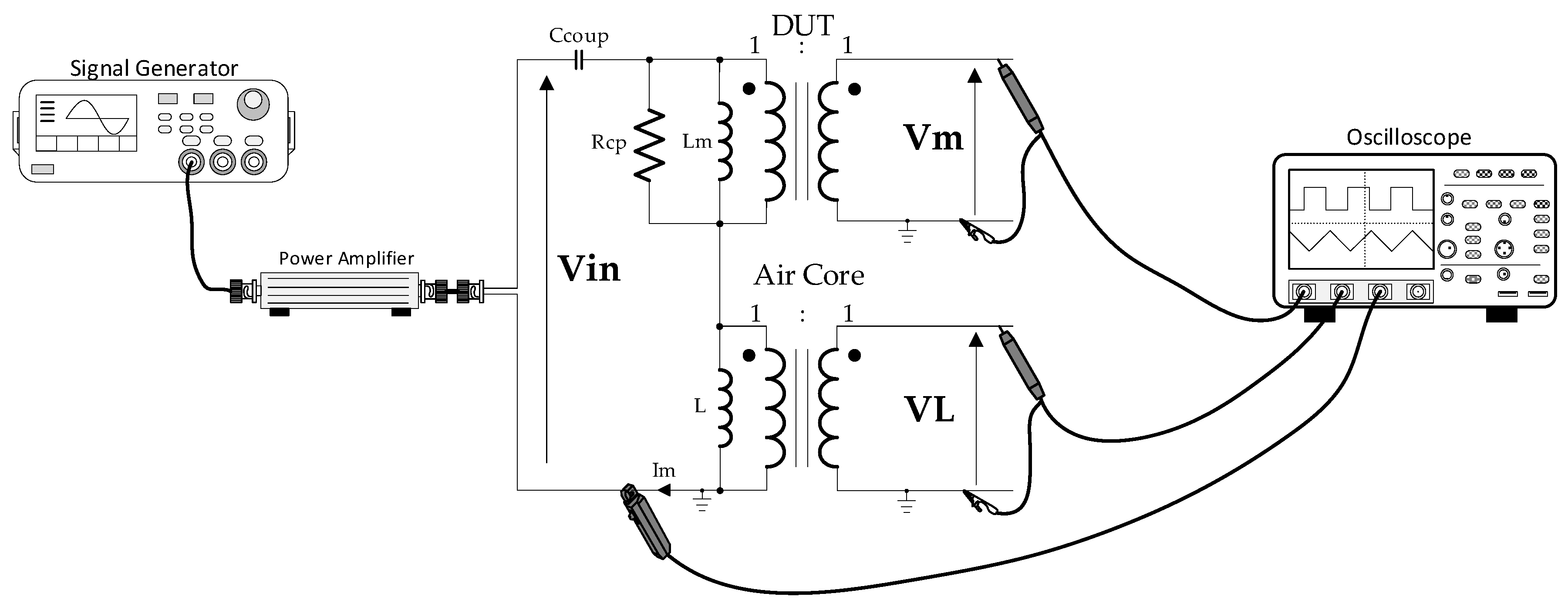
5. Test-Bench Measurement and Verification

The test-bench measurement and verification have been done on three toroidal inductors using cores made by Ferroxcube. These are TN10/6/4−3C90—Sample 1, TN10/6/4−3C94—Sample 2, and TN13/7.5/5−3F3—Sample 3 wound, with three turns bifilar winding made of DNE 0.65 copper wire as shown in Figure 12a–c. The air core transformer was constructed using a TN58/18/9—Air Trafo non-magnetic core made of ABS plastic, featuring 10 turns of bifilar winding made from DNE 0.65 mm copper wire, as shown in Figure 12d.

The switching frequencies of the testing setup have been chosen to be 100 kHz, 200 kHz, and 300 kHz, respectively, which are typical values for modern SMPSs and also the recommended values by the core manufacturers for each of the tested core materials.

The main test-bench setup is shown in Figure 13a–d. It consisted of a 12-bit LeCroy HDO6104-MS 1 GHz oscilloscope, a Rigol DG992 SiFi II 2-channel 100 MHz arbitrary signal generator, a Rigol DM3068 digital multimeter, a Rigol DP832A programmable DC power supply, and a FPA301−20W 10 MHz function generator amplifier. The voltage signals were measured using two TESTEC TT-LX 312 voltage probes. while the current was measured by the LeCroy CP031A current probe.

As shown in Figure 13d, the inductors under test were submerged in an oil bath to heat them up to the required temperature and then keep them constant at this state. Moreover, the oil bath has been further encapsulated within a plastic container for additional temperature insulation, fume removal, and to facilitate a close setup of the remaining circuitry to the inductor, as shown in Figure 13b. The temperature control has been implemented using an Arduino platform, along with the set of relays, as shown in Figure 13c. The Arduino used a DS18B20 sensor to monitor and adjust the temperature variations and it has been synchronized with a K-type thermocouple used by the Rigol DM 3068 as a reference. This setup allowed to keep the constant temperature within ±2 °C. The circuit schematic of the test-bench is shown in Figure 14.

As can be seen in Figure 14, instead of using a current sensing resistor that might introduce significant phase discrepancy between the primary magnetizing current $i_m$ and the secondary side magnetizing voltage $V_m$ of the inductor under test, the LeCroy CP031A current probe has been used. The current probe has a 1 mA/Div sensitivity, an amplitude accuracy of $\pm 1\%$ of reading, a measurement range of up to 30 A, and a 100 MHz bandwidth, features that outperform any current sensing resistor measurement methodology. Moreover, to limit the possible phase discrepancy between the primary magnetizing current $i_m$ and the inductor secondary side magnetizing voltage $V_m$, the current probe has been deskewed with the voltage probes using the LeCroy DCS015 deskewing fixture.

The voltage probes themselves have been deskewed amplitude-wise and phase discrepancy-wise by measuring the same voltage of 2 V peak-to-peak value with 50 ns rising/falling slopes and 50% duty-cycle ratio at 500 kHz switching frequency using both (i) a Rigol DG992 SiFi II signal generator, and (ii) as it was described in Section 2, by measuring the same voltage and then calculating an integral ${\displaystyle \frac{1}{T}}{\int }_0^T{v}_m^{\prime }{i}_{m}dt$ for each of them. The results were adjusted using deskew functions in the oscilloscope until the calculated integrals showed the same value.

The coupling capacitor $C_{coup}$ has been chosen as a set of capacitors connected in parallel to maintain a constant DC blocking value at various excitation levels and limit the parasitic resistance introduced by it below 100 mΩ at switching frequencies ranging from 100 kHz to 300 kHz.

The values of the inductor under test and the air core transformer inductances have been chosen as a trade-off between the measurement accuracy and the limitation of the switching noise introduced by the inductors’ inductances themselves as well as their parasitic capacitances. The further limitation of the switching noise has been done by the limitation of the square waveform excitation signal slew rate to 50 ns on both signal edges. The detailed parameters of the tested inductors and air-core transformer have been obtained using a Bode 100 impedance analyzer and are presented in

Table 1. Parameters of inductors under test and air core transformer at 25 °C and 10 kHz.

Description	Core	Material	N	Lprim [μH]	Lsec [μH]	Lleak_prim [nH]	Lleak_sec [nH]	Rleak_prim [mΩ]	Rleak_sec [mΩ]	Cinter_wind [pF]	Rcp [Ω]	fres [MHz]
Sample 1	TN10/6/4	3C90	3	8.184	8.058	239.665	238.684	23.727	17.093	14.751	107.427	16.492
Sample 2	TN10/6/4	3C94	3	9.719	9.751	249.976	236.226	13.048	12.855	12.903	111.939	11.543
Sample 3	TN13/7.5/5	3F3	3	9.736	9.620	172.545	183.281	11.306	10.078	12.454	128.580	8.201
Air Trafo	TN58/18/9	Air	10	0.476	0.476	395.626	371.912	24.617	29.967	25.676	-	100

at 25 °C/10 kHz and in

Table 2. Parameters of inductors under test and air core transformer at 100 °C and 10 kHz.

Description	Core	Material	N	Lprim [μH]	Lsec [μH]	Lleak_prim [nH]	Lleak_sec [nH]	Rleak_prim [mΩ]	Rleak_sec [mΩ]	Cinter_wind [pF]	Rcp [Ω]	fres [MHz]
Sample 1	TN10/6/4	3C90	3	18.376	18.307	189.042	191.497	21.881	22.56	78.647	150.708	4.800
Sample 2	TN10/6/4	3C94	3	11.708	11.288	182.671	199.912	23.270	21.437	95.059	148.843	7.368
Sample 3	TN13/7.5/5	3F3	3	17.931	17.878	196.525	171.681	26.126	24.991	27.125	171.068	4.722
Air Trafo	TN58/18/9	Air	10	-	-	-	-	-	-	-	-	-

where ${\mathrm{L}}_{\mathrm{p}\mathrm{r}\mathrm{i}\mathrm{m}}$—primary side inductance with secondary side open, ${\mathrm{L}}_{\mathrm{s}\mathrm{e}\mathrm{c}}$—secondary side inductance with primary side open, ${\mathrm{L}}_{\mathrm{l}\mathrm{e}\mathrm{a}\mathrm{k}\_\mathrm{p}\mathrm{r}\mathrm{i}\mathrm{m}}$—primary side leakage inductance with secondary side shorted, ${\mathrm{L}}_{\mathrm{l}\mathrm{e}\mathrm{a}\mathrm{k}\_\mathrm{s}\mathrm{e}\mathrm{c}}$—secondary side leakage inductance with primary side shorted, ${\mathrm{R}}_{\mathrm{l}\mathrm{e}\mathrm{a}\mathrm{k}\_\mathrm{p}\mathrm{r}\mathrm{i}\mathrm{m}}$—primary side leakage resistance with secondary side shorted, ${\mathrm{R}}_{\mathrm{l}\mathrm{e}\mathrm{a}\mathrm{k}\_\mathrm{s}\mathrm{e}\mathrm{c}}$—secondary side leakage resistance with primary side shorted, ${\mathrm{C}}_{\mathrm{i}\mathrm{n}\mathrm{t}\mathrm{e}\mathrm{r}\_\mathrm{w}\mathrm{i}\mathrm{n}\mathrm{d}}$—interwinding capacitance with primary and secondary side shorted, ${\mathrm{R}}_{\mathrm{c}\mathrm{p}}$—core parallel resistance measured as the value of impedance at inductor self-resonance, ${\mathrm{f}}_{\mathrm{r}\mathrm{e}\mathrm{s}}$—frequency at inductor self-resonance.

at 100 °C/10 kHz.

Moreover, the further reduction of any unwanted noise or floating potential has been achieved by connecting the oscilloscope, the signal generator, the DC power supply, the primary and secondary side of the inductors under test, and the air transformer to the same ground plane, as shown in Figure 13 and Figure 14, respectively.

All data processing was performed in the LTSpice 24.1.9 simulator.

5.1. Reversible Permeability Measurement

STEP I

The calculations start with establishing small- and large-signal reversible permeability roll-off required to estimate the $\sigma$ and $\eta$ coefficients shown in Equation (37). These coefficients will be used to adjust the OSE calculations when the excitation signal goes into the non-linear region.

First, the B–H characteristics of each of the inductors must be measured at 25 °C and 100 °C, respectively. Because the anhysteretic curve was assumed to be frequency invariant, the calculations were based on the B–H curves captured at 100 kHz only. As shown in Figure 15a–c, the lowest testing frequency means lower inductor impedance, and thus higher to achieve magnetic field intensity values and more visible saturation effects. The characteristics reach different values at negative and positive far ends. This is due to the FPA301−20W signal amplifier’s limitations, as it works beyond its nominal range under these conditions, while the small jump visible in the characteristics near the positive coercive field value is due to the reset of the voltage integral in LTSpice.

The calculations of reversible permeability were split into two parts. The small-signal reversible permeability ${\mu }_{rev}$ is used to adjust calculations during DC bias premagnetization and is based on the approach by Esguerra et al. [25,26,27,28,29]. The large-signal reversible permeability ${\mu }_{rev\left(a\right)}$ adjusts the calculations if the excitation signal reaches the B–H curve non-linear region and is based on an iterative approach measuring the changes of B and H along the B–H curve at each adjacent step where the B–H curve measurement was performed. The fitting coefficients for the Esguerra et al. approach at 25 °C and 100 °C are given in

Table 3. Esguerra et al. fitted coefficients at 25 °C.

Description	${\mathit{\mu }}_{\mathit{c}}$	${\mathit{\mu }}_{\mathit{i}}$	a	${\mathit{\alpha }}_0$	Bsat [T]
Sample 1	5627	2120	3.48	10.05	0.48
Sample 2	7236	2639	1.84	9.06	0.46
Sample 3	6464	1963	2.83	12.84	0.51

and

Table 4. Esguerra et al. fitted coefficients at 100 °C.

Description	${\mathit{\mu }}_{\mathit{c}}$	${\mathit{\mu }}_{\mathit{i}}$	a	${\mathit{\alpha }}_0$	Bsat [T]
Sample 1	6778	5070	3.22	2.56	0.36
Sample 2	4187	3235	3.73	2.69	0.37
Sample 3	6939	3975	2.89	4.86	0.41

where ${\mu }_c$ is a large-signal permeability measured at the coercive field; ${\mu }_i$ is an initial small-signal permeability measured by Bode 100 at 10 kHz; and $a, {\alpha }_0, { B}_{sat}$ are the fitting coefficients.

, respectively.

In general, the relative values of both permeability roll-offs show similar behavior at 100 °C as shown in Figure 16a–c.

Because calculations of the original Steinmetz equation (OSE) involve temperature adjustments, knowledge of the change in the large-signal relative permeability roll-off with temperature is also required. This is illustrated in Figure 17a–c for 25 °C and 100 °C, respectively. The difference between these values is linearly interpolated in calculations.

Having the above data already analyzed, it is possible now to estimate the $\sigma$ and $\eta$ shown in Equation (37) and go to STEP II–IV.

5.2. Original Steinmetz Equation Coefficients

STEP II–III

The core power loss and the coefficients describing the OSE equation have been measured at $100 °\mathrm{C},$ placing the inductors under test in the heated oil bath. The value of the magnetic flux density was extracted from the $V_m$ inductor voltage of sinusoidal shape by integration of the measured signal in LTSpice. The switching frequencies were set to 100 kHz, 200 kHz, and 300 kHz, respectively.

At this stage, there was no DC component in the excitation signals, and thus, the $\sigma$ coefficient was set to 1.0, while the $\eta$ coefficient was set accordingly to the amplitude of the magnetic flux density and the reversible permeability change as shown in Figure 17a–c. The coefficient fitting was done using an Excel Solver and the least squares method.

The STEP III was conducted in a similar manner where the temperature of tested inductors was swept from $25 °\mathrm{C}$ to $120 °\mathrm{C}$ at magnetic flux density swing of 100 mT at 100 kHz and 50 mT at 200 kHz and 300 kHz, respectively. The fitting of a fifth-degree polynomial was done this time in the OriginLab software (Version 10.0.0.154).

The power loss measurement results are shown in Figure 18a–f overlaid on the power loss characteristics taken directly from the manufacturer’s datasheets for reference. The fitting coefficients are shown in

Table 5. Sample 1 OSE and temperature fitting coefficients.

Description	${\mathit{f}}_{\mathit{s}}\left[\mathbf{k}\mathbf{H}\mathbf{z}\right]$	$\mathit{k}$	$\mathit{\alpha }$	$\mathit{\beta }$	${\mathit{\xi }}_5$	${\mathit{\xi }}_4$	${\mathit{\xi }}_3$	${\mathit{\xi }}_2$	${\mathit{\xi }}_1$	${\mathit{\xi }}_0$
Sample 1	100	0.791	1.529	2.629	−2.45 × 10−9	8.91 × 10−7	−1.20 × 10−4	0.0076	−0.25586	5.515
	200	0.904	1.504	2.525	−1.94 × 10−9	7.29 × 10−7	−1.02 × 10−4	0.0068	−0.23982	5.322
	300	0.970	1.485	2.393	−2.18 × 10−9	8.40 × 10−7	−1.21 × 10−4	0.0083	−0.27899	5.234

,

Table 6. Sample 2 OSE and temperature fitting coefficients.

Description	${\mathit{f}}_{\mathit{s}}\left[\mathbf{k}\mathbf{H}\mathbf{z}\right]$	$\mathit{k}$	$\mathit{\alpha }$	$\mathit{\beta }$	${\mathit{\xi }}_5$	${\mathit{\xi }}_4$	${\mathit{\xi }}_3$	${\mathit{\xi }}_2$	${\mathit{\xi }}_1$	${\mathit{\xi }}_0$
Sample 2	100	0.848	1.581	2.761	−6.01 × 10−10	2.30 × 10−7	−3.20 × 10−5	0.00227	−0.09287	2.644
	200	0.810	1.540	2.508	−5.91 × 10−10	2.11 × 10−7	−2.80 × 10−5	0.00195	−0.0823	2.418
	300	0.838	1.533	2.461	−3.49 × 10−10	1.06 × 10−7	−1.09 × 10−5	6.01 × 10−4	−0.02716	1.553

, and

Table 7. Sample 3 OSE and temperature fitting coefficients.

Description	${\mathit{f}}_{\mathit{s}}\left[\mathbf{k}\mathbf{H}\mathbf{z}\right]$	$\mathit{k}$	$\mathit{\alpha }$	$\mathit{\beta }$	${\mathit{\xi }}_5$	${\mathit{\xi }}_4$	${\mathit{\xi }}_3$	${\mathit{\xi }}_2$	${\mathit{\xi }}_1$	${\mathit{\xi }}_0$
Sample 3	100	0.811	1.547	2.704	−2.51 × 10−9	8.77 × 10−7	−1.12 × 10−4	0.00681	−0.22914	5.049
	200	0.709	1.571	2.769	−2.54 × 10−9	8.87 × 10−7	−1.15 × 10−4	0.00729	−0.25979	5.875
	300	0.826	1.503	2.421	−2.27 × 10−9	8.18 × 10−7	−1.10 × 10−4	0.00703	−0.23142	4.443

where $f_s$ is the switching frequency.

, respectively.

As shown in Figure 18a–f, the data obtained from the manufacturers’ datasheets and the test-bench measurements are consistent for 3C90 and 3F3 but differ significantly for 3C94. This is likely due to high material spreads during the manufacturing process and shows how important material verification is before any mass production of any magnetic components. This should mainly involve the Monte Carlo analysis.

5.3. Unified Small and Large-Signal Core Loss Model

STEP IV

As stated in [18] and Section 3 of this work, there are two concurrent core loss models, depending on the magnitude of the excitation signals that exclude one another. As shown in Figure 10, the large-signal OSE model smoothly transitions to the small-signal complex permeability model at low levels of excitation, and the core resistance characteristics flatten out. So, the unification of both models seems to be imminent both (i) because that is how the inductor really behaves, and (ii) because the single model can be used in both small- and large-signal domains, which was not possible before helping, e.g., in the design of the low-noise magnetic shielding [22].

The core resistance characteristics extraction procedure was performed using a Bode 100 impedance analyzer. To do so, the impedance of the tested inductor was measured at various levels of excitation signals ranging from $0.1 \mathrm{m}\mathrm{T}$ to $20 \mathrm{m}\mathrm{T}$. During the measurement, the voltage and current were captured using the TESTEC TT-LX 312 and the LeCroy CP031 probes. The voltage probe was connected to the secondary side of the tested inductor to avoid the introduction of any unwanted parasitic effects at the primary side during measurement.

The real part of the impedance measurement consists of core resistance, winding resistance, and a combination of other parasitic effects, which are discussed in Section 3.1. Therefore, the core resistance must be separated from the remaining unwanted components. Regarding the inductors that are wound with several winding turns, the winding resistance is affected by the magnetic field existing around the core [18]. Thus, the separation process can be performed using the Dowell equation, aided by the small signal inductor model and the complex permeability iterative approximation method, as shown in [21].

However, in the case of the tested inductors, the real part of the impedance measurement is mainly affected by the resistance of the winding wires and the soldering joints because, as shown in Figure 12a–c, only a small portion of the windings is wound around the core. The structure of the windings is done that way since the inductor must be submerged deep enough into the oil bath and at the same time be connected to the remaining testing circuitry as shown in Figure 13a–d. Moreover, three turns of bifilar windings are a trade-off between the magnetic field distribution around the core and the limitation of significant inductance introduced into the switching circuitry, which helps avoid unwanted oscillations during switching.

Therefore, instead of using the method described in [21], it was assumed that the winding resistance can be measured on a dummy core of equivalent size, made of ABS plastic and wound with equivalent winding wire. This resistance was then subtracted from the real part of the measured impedance, giving the core resistance only. Examples of the results for 100 kHz, 200 kHz, and 300 kHz are shown in Figure 19a–c.

As one might expect, the transition between the small- and large-signal core resistance models does not occur smoothly as presented in Figure 19a–c. The visible deviation from that can be seen in Figure 20.

The reason for that might be a complex case. First, the Steinmetz core loss model is simplified by a straight line in the linear domain up to 300 mT. This model is typically fitted with a certain level of accuracy as shown in Section 5.2. Initially, this introduces some deviations in the prediction of the characteristics’ slope at different excitation levels. Second, the Steinmetz model might not be a straight line after all but rather a segmented one, as shown in the ferrite magnetic design tool provided by TDK [34]. In this case, the measured core loss is not tangential to the Steinmetz-based predicted values due to dispersion in the characteristics slope estimation. Third, in Equation (39), repeated here for convenience:

$$R_c=2V_{e}k{f}^{\alpha }{B}_m^{\beta }{\widehat{I}}_m^{-2}\left(\sum _{n=0}^5{\xi }_n{T}^n\right)$$

(45)

The core resistance is a function of two variables: the $B_m$ and the $I_m$, while the $I_m$ does not exist in the original Steinmetz core loss prediction. Therefore, the $I_m$ was measured during the Bode 100 impedance sweep and introduced to the model. This results in the $R_c\left(I_m\right)$ characteristic shown in Figure 19a–c and Figure 20, respectively. It can be seen that this characteristic more closely follows the measured values of $R_c$ at higher excitation signals. Additionally, the Equation (45) can be rewritten in the linear region to:

$$R_c=2V_{e}k{f}^{\alpha }{B}_m^{\beta }{\left({\displaystyle \frac{B_{m}N{A}_c}{L}}\right)}^{-2}\left(\sum _{n=0}^5{\xi }_n{T}^n\right)$$

(46)

where $N$ is a number of winding turns, $A_c$ is an effective cross-section area of the magnetic core, and $L$ is the inductance. In this case, the values of $L$ can be directly taken from the impedance measurement. This approach gives the most consistent results compared to the measured characteristics. Fourth, as previously stated, the winding resistance was measured on a dummy core and assumed to be invariant to the excitation level. Moreover, the inductor parasitics, which contribute to the real and imaginary parts of the impedance, were also neglected. This may also be a cause of the small-signal core resistance characteristics bending phenomenon, which existing core loss models do not predict.

Finally, the impedance analyzer used for the measurements has a limited range of excitation signal amplitudes. At the current setup of the tested inductors and the assumed switching frequencies, it could reach only 20 mT. Therefore, some simplifications were necessary regarding the core resistance fitting procedure. It was then assumed that the value of inductance in Equation (46) is an average one, being the mean value of all inductances measured by the impedance analyzer. This is represented by the $R_c\left(L_{avg}\right)$ characteristics shown in Figure 19a–c and Figure 20, respectively. Unifying the small- and large-signal core loss model, Equation (46) becomes:

$$R_c=2V_{e}k{f}^{\alpha }\left(B_m^{\beta }+\sum _{i=0}^9{\chi }_i{B}_m^i\right){\left({\displaystyle \frac{B_{m}N{A}_c}{L_{avg}}}\right)}^{-2}\left(\sum _{n=0}^5{\xi }_n{T}^n\right)$$

(47)

where ${\chi }_i$ are the fitting coefficients of the ninth-degree polynomial used to combine small and large signal core loss characteristics. The values of $L_{avg}$ are given in

Table 8. The average value of inductance during small- and large-signal core resistance fitting.

Description	${\mathit{f}}_{\mathit{s}}\left[\mathbf{k}\mathbf{H}\mathbf{z}\right]$	Sample 1	Sample 2	Sample 3
$L_{avg} \left[\mu H\right]$	100	7.497	8.672	8.365
	200	7.454	8.741	8.467
	300	7.623	7.622	8.749

.

The ${\left(\frac{B_{m}N{A}_c}{L_{avg}}\right)}^{-2}$ expression can now be treated as a constant, allowing the transformation of the core resistance given by Equation (47) back to the core loss given by Equation (40).

The values of the ninth-degree polynomial are given in

Table 9. Sample 1 ninth-degree polynomial coefficients.

Description	${\mathit{f}}_{\mathit{s}}\left[\mathit{k}\mathit{H}\mathit{z}\right]$	${\mathit{\chi }}_9$	${\mathit{\chi }}_8$	${\mathit{\chi }}_7$	${\mathit{\chi }}_6$	${\mathit{\chi }}_5$	${\mathit{\chi }}_4$	${\mathit{\chi }}_3$	${\mathit{\chi }}_2$	${\mathit{\chi }}_1$	${\mathit{\chi }}_0$
Sample 1	100	−725.08	1025.98	−609.21	197.11	−37.45	4.17	−0.25239	0.00638	2.22 × 10−8	−1.70 × 10−13
	200	−733.34	1020.17	−595.92	189.24	−35.24	3.84	−0.22725	0.00561	1.43 × 10−7	−8.50 × 10−13
	300	−599.28	847.12	−503.48	162.89	−30.94	3.45	−0.20846	0.00527	2.47 × 10−7	−1.19 × 10−12

,

Table 10. Sample 2 ninth-degree polynomial coefficients.

Description	${\mathit{f}}_{\mathit{s}}\left[\mathbf{k}\mathbf{H}\mathbf{z}\right]$	${\mathit{\chi }}_9$	${\mathit{\chi }}_8$	${\mathit{\chi }}_7$	${\mathit{\chi }}_6$	${\mathit{\chi }}_5$	${\mathit{\chi }}_4$	${\mathit{\chi }}_3$	${\mathit{\chi }}_2$	${\mathit{\chi }}_1$	${\mathit{\chi }}_0$
Sample 2	100	−631.83	879.29	−513.85	163.25	−30.42	3.32	−0.1964	0.00486	2.55 × 10−8	−1.69 × 10−13
	200	−733.34	1020.17	−595.93	189.24	−35.24	3.84	−0.22725	0.00561	1.43 × 10−7	−8.50 × 10−13
	300	−1708.83	2414.73	−1434.67	464.00	−88.12	9.82	−0.59329	0.015	1.67 × 10−7	−8.71 × 10−13

, and

Table 11. Sample 3 ninth-degree polynomial coefficients.

Description	${\mathit{f}}_{\mathit{s}}\left[\mathbf{k}\mathbf{H}\mathbf{z}\right]$	${\mathit{\chi }}_9$	${\mathit{\chi }}_8$	${\mathit{\chi }}_7$	${\mathit{\chi }}_6$	${\mathit{\chi }}_5$	${\mathit{\chi }}_4$	${\mathit{\chi }}_3$	${\mathit{\chi }}_2$	${\mathit{\chi }}_1$	${\mathit{\chi }}_0$
Sample 3	100	−249.76	351.26	−207.63	66.79	−12.61	1.39	−0.08386	0.00211	2.78 × 10−8	−1.66 × 10−13
	200	−587.67	829.69	−492.48	159.12	−30.19	3.36	−0.2028	0.00512	1.55 × 10−8	−9.35 × 10−14
	300	−206.99	287.063	−167.11	52.86	−9.80	1.06	−0.06253	0.00153	2.63 × 10−7	−1.42 × 10−12

, respectively, while the fitted $R_C Fitted$ characteristics are shown in Figure 19a–c and Figure 20, respectively. The fitting was performed using OriginLab software.

The imaginary part of the complex permeability $\mu ″$ values used to calculate the core resistance that is based on the small-signal complex permeability model was estimated based on the values of core resistance at which the $R_c Measured$ characteristics bend horizontally, as shown in Figure 19a–c and Figure 20, respectively. These values are in good agreement with the IEC 62044−2 standard and correspond to the values at which magnetic flux density $B_m$ stays within a range of $0.17 \mathrm{m}\mathrm{T}\pm 0.22 \mathrm{m}\mathrm{T}$, which is below the required value of $0.25 \mathrm{m}\mathrm{T}$ according to the IEC 62044−2 standard.

5.4. Rectangular and Sinusoidal Excitations with a DC Bias

STEP V

As stated in Section 4, there are a few scenarios possible in this step, namely:

5.4.1. Sinusoidal Excitation with DC Bias Characteristics—STEP V.1.

The DC bias was introduced into the test bench by adding a DC voltage source in series with a 1 mH inductor [7,11,14,16,17]. The inductor transferred the DC bias voltage into the DC bias current used in the pre-magnetization of the core. The modified test-bench circuit schematic is shown in Figure 21.

The added inductor has a self-resonance at 1.3 MHz, which is sufficiently high to keep the inductance stable at the switching frequencies of the test.

Because the DC pre-magnetization was done by an introduction of a DC bias current, the core loss of the tested inductors with the DC pre-magnetization was a function of the magnetic field strength $P_c\cdot F\left(H_{dc}\right)$ rather than a function of the magnetic flux density $P_c\cdot F\left(B_{dc}\right)$. So, the sinusoidal $P_c\cdot F\left(H_{dc}\right)$ was transferred into the $P_c\cdot F\left(B_{dc}\right)$ to obtain a function of only one variable $B$ as in Equation (41). This was achieved using an iterative approximation curve fitting method similar to that described in [21], with coefficients provided in Table 4. The measurement results are given in Figure 22a–f.

The magnetic flux density swing was set to B_m = 100 mT at 100 kHz and B_m = 50 mT at 200 kHz and 300 kHz, respectively.

During the test-bench measurements, the $\sigma$ coefficient, as shown in Equation (37), was calculated based on the characteristics given in Figure 16a–c, while the $\eta$ coefficient depended on the magnitude of the magnetic flux density swing and was based on the characteristics shown in Figure 16a–c and Figure 17a–c, respectively. Fitting coefficients are given in

Table 12. Sample 1 $P_c\cdot F\left(B_{dc}\right)$ fourth-degree polynomial coefficients.

Description	${\mathit{f}}_{\mathit{s}}\left[\mathbf{k}\mathbf{H}\mathbf{z}\right]$	${\mathit{\zeta }}_4$	${\mathit{\zeta }}_3$	${\mathit{\zeta }}_2$	${\mathit{\zeta }}_1$	${\mathit{\zeta }}_0$
Sample 1	100	−370.118	199.123	−5.470	−2.5174	1.0098
	200	−186.883	232.729	−10.233	−4.0389	0.9487
	300	99.271	66.133	−3.080	−2.4056	0.9731

,

Table 13. Sample 2 $P_c\cdot F\left(B_{dc}\right)$ fourth-degree polynomial coefficients.

Description	${\mathit{f}}_{\mathit{s}}\left[\mathbf{k}\mathbf{H}\mathbf{z}\right]$	${\mathit{\zeta }}_4$	${\mathit{\zeta }}_3$	${\mathit{\zeta }}_2$	${\mathit{\zeta }}_1$	${\mathit{\zeta }}_0$
Sample 2	100	684.753	−354.010	78.725	−6.8433	1.0029
	200	150.945	83.041	25.125	−8.408	1.0161
	300	−148.965	80.326	7.861	−3.3445	0.9999

, and

Table 14. Sample 3 $P_c\cdot F\left(B_{dc}\right)$ fourth-degree polynomial coefficients.

Description	${\mathit{f}}_{\mathit{s}}\left[\mathbf{k}\mathbf{H}\mathbf{z}\right]$	${\mathit{\zeta }}_4$	${\mathit{\zeta }}_3$	${\mathit{\zeta }}_2$	${\mathit{\zeta }}_1$	${\mathit{\zeta }}_0$
Sample 3	100	−449.625	188.253	1.674	−0.7833	1.0291
	200	−1136.548	667.751	−71.603	−0.4124	0.9818
	300	−224.727	179.503	−12.493	−1.4470	1.0019

, respectively.

The characteristics fitting was done using an Excel Solver.

5.4.2. Rectangular Excitation with a DC Bias Characteristics—STEP V.2.

If rectangular excitation occurred, the corresponding core loss was calculated using Equation (42). The measured power loss characteristics are shown in Figure 23a–c.

During the core loss measurement, the duty-cycle was swept from 0.1 to 0.9 at corresponding magnetic flux densities and switching frequencies, which are B_m = 100 mT at 100 kHz and B_m = 50 mT at 200 kHz and 300 kHz, respectively. The $\sigma$ coefficient was set to 1.0 because there was not a DC bias, and the $\eta$ was set according to the amplitude of magnetic flux density swing, as shown in Figure 16a–c and Figure 17a–c, respectively. The measurement was done at 100 °C.

The fitting coefficients of the function described by Equation (42) are given in

Table 15. Complete iRESE model fitting coefficients STEP V.2.

Description	${\mathit{f}}_{\mathit{s}}\left[\mathbf{k}\mathbf{H}\mathbf{z}\right]$	$\mathit{\gamma }$	$\mathit{\delta }$
Sample 1	100	0.8465	0.8512
	200	0.9226	0.9771
	300	0.8205	0.9794
Sample 2	100	0.7525	0.8510
	200	0.9847	0.9209
	300	0.8751	0.9401
Sample 3	100	0.7947	0.9028
	200	1.1165	1.0270
	300	1.0206	1.0089

. They were estimated with the assumption that the $B_{dc}=0$, and the fitting itself was done using an Excel Solver.

The examples of the captured waveforms in the LTSpice format for Sample 1 at 300 kHz and duty-cycles of $D=0.5$ and $D=0.1$ are shown in Figure 24a–b, respectively.

5.4.3. Rectangular Excitation Without a DC Bias—STEP V.3.

If there is no DC bias and a rectangular excitation takes place, the core loss is expressed by Equation (43). The same power loss characteristics as shown in Figure 23a–c apply. The fitting coefficients are given in

Table 16. Rectangular excitation fitting coefficients without a DC bias—STEP V.3.

Description	${\mathit{f}}_{\mathit{s}}\left[\mathbf{k}\mathbf{H}\mathbf{z}\right]$	${\mathit{\gamma }}_1$	${\mathit{\delta }}_1$
Sample 1	100	0.8465	0.8596
	200	0.9226	0.9271
	300	0.8205	0.9531
Sample 2	100	0.752	0.8535
	200	0.9847	0.9365
	300	0.8751	0.9401
Sample 3	100	0.7947	0.9028
	200	1.1165	1.0270
	300	1.0206	1.0109

.

As might be expected, the fitting coefficients in Table 16 have almost the same values as the coefficients given in Table 15 at $B_{dc}=0.$ The slight differences come from the fitting of the $F\left(B_{dc}\right)$ function, which is expected.

5.4.4. Rectangular Excitation with a DC Bias Characteristics—STEP V.4.

If rectangular excitation comes together with the DC bias, the DC bias is added to the core loss with the assumption that the duty-ratio of the signals’ equals $D=0.5$. Since a complex relationship exists between B and H near the core saturation region, if rectangular excitation takes place, the DC magnetization function to be added is left to be a function of $H_{dc}$ than $B_{dc}$, as in Equations (41) and (42).

The power loss characteristics are shown in Figure 25a–c.

In these measurements, the $\sigma$ coefficient of Equation (37) was set according to the DC value of the magnetic field strength H, while the $\eta$ coefficient according to the peak of the magnetic flux density swing $B_m$ as shown in Figure 16a–c and Figure 17a–c, respectively.

The peak of the magnetic flux swing (the variable component) was set as in previous cases as follows: Bm = 100 mT at 100 kHz, Bm = 50 mT at 200 kHz and 300 kHz, respectively.

Fitting coefficients are given in

Table 17. Sample 1 $P_c\cdot F\left(H_{dc}\right)$ fourth-degree polynomial coefficients.

Description	${\mathit{f}}_{\mathit{s}}\left[\mathbf{k}\mathbf{H}\mathbf{z}\right]$	${\mathit{ϵ}}_4$	${\mathit{ϵ}}_3$	${\mathit{ϵ}}_2$	${\mathit{ϵ}}_1$	${\mathit{ϵ}}_0$
Sample 1	100	1.15 × 10−6	−0.0001627	0.007439	−0.08603	1.0606
	200	1.15 × 10−6	−0.0001679	0.008528	−0.11997	1.1115
	300	6.07 × 10−8	−0.0000184	0.001820	−0.03518	1.0186

,

Table 18. Sample 2 $P_c\cdot F\left(H_{dc}\right)$ fourth-degree polynomial coefficients.

Description	${\mathit{f}}_{\mathit{s}}\left[\mathbf{k}\mathbf{H}\mathbf{z}\right]$	${\mathit{ϵ}}_4$	${\mathit{ϵ}}_3$	${\mathit{ϵ}}_2$	${\mathit{ϵ}}_1$	${\mathit{ϵ}}_0$
Sample 2	100	1.00 × 10−6	−0.0001296	0.0056645	−0.08053	1.1350
	200	1.00 × 10−6	−0.0001325	0.0064732	−0.10974	1.1437
	300	−1.72 × 10−8	2.94 × 10−8	0.0004832	−0.02038	1.0186

, and

Table 19. Sample 3 $P_c\cdot F\left(H_{dc}\right)$ fourth-degree polynomial coefficients.

Description	${\mathit{f}}_{\mathit{s}}\left[\mathbf{k}\mathbf{H}\mathbf{z}\right]$	${\mathit{ϵ}}_4$	${\mathit{ϵ}}_3$	${\mathit{ϵ}}_2$	${\mathit{ϵ}}_1$	${\mathit{ϵ}}_0$
Sample 3	100	1.15 × 10−6	−0.0001478	0.0062136	−0.05208	1.0729
	200	1.15 × 10−6	−0.0001458	0.0074738	−0.12003	1.1337
	300	6.07 × 10−8	−0.0000214	0.0018027	−0.02333	1.0186

, respectively.

The characteristics fitting was done using an Excel Solver.

Moreover, there may be some differences in results regarding the functions described by Equations (42) and (44). This is because, as shown in Figure 2, the losses excited by the rectangular signal at duty-ratio of 0.5 were lower than the losses excited by the sinusoidal signal at the same amplitude of the magnetic flux density. An example of this phenomenon is shown in Figure 26.

The cancellation factor $k$ introduced in Section 2 and shown in Equation (37) in all measurements regarding sinusoidal and rectangular excitations was calculated according to Equation (11). It was done by the introduction of $1°$ perturbation into $i_m$ signal because this method (i) introduces only a 1% discrepancy to the measurements described in Section 5.4.2 and Section 5.4.3, and (ii) solves the problem with perturbed $v_L$ signal at high DC bias values; otherwise, it was introduced into calculations using Equation (13).

6. Error Analysis

The error analysis identifies potential sources of measurement errors in the test-bench system. The identification of these errors is crucial for a better understanding of possible measurement discrepancies and their magnitude in relation to the obtained results. Moreover, the error analysis indicates whether the assumed measurement approach and the test-bench setup are suitable for the expected measurement accuracy and make sense.

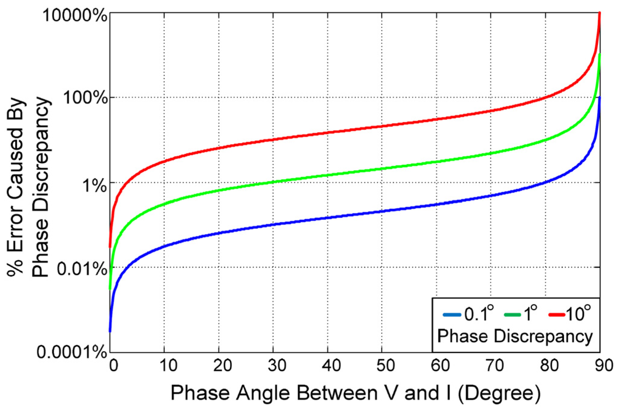
6.1. Oscilloscope Measurement Errors

The LeCroy HDO6104-MS 1 GHz oscilloscope features a 12-bit vertical resolution, providing 4096 Q levels (0.195 mV), which is significantly better than the eight-bit oscilloscopes having only 256 Q levels (3.125 mV). When only the least significant bit of the oscilloscope ADC converter is considered, the measurement error caused by the amplitude discrepancy is 0.012%, which could be easily neglected.

As stated in Section 5 and as it can be seen in Figure 14, instead of using a current sensing resistor that might introduce significant phase discrepancy between the primary magnetizing current $i_m$ and the secondary side magnetizing voltage $V_m$ of the inductor under test, the LeCroy CP031A current probe has been used. The current probe has a 1mA/Div sensitivity, an amplitude accuracy of $\pm 1\%$ of reading, a measurement range of up to 30 A, and a 100 MHz bandwidth, features that outperform any current sensing resistor measurement method. Moreover, to limit the possible phase discrepancy between the primary magnetizing current $i_m$ and the inductor secondary side magnetizing voltage $V_m$, the current probe has been deskewed with the voltage probe using the LeCroy DCS015 deskewing fixture. The CP031A has an insertion impedance of only 0.012 Ω at 300 kHz, which, again, outperforms any resistor-based current sensing approach.

The voltage probes themselves have been deskewed amplitude-wise and phase discrepancy-wise by measuring the same voltage of 2 V peak-to-peak value with 50 ns rising/falling slopes and 50% duty-cycle ratio at 500 kHz switching frequency using both (i) the Rigol DG992 SiFi II signal generator, and (ii) as it was described in Section 2, by measuring the same voltage and then calculating an integral ${\displaystyle \frac{1}{T}}{\int }_0^T{v}_m^{\prime }{i}_{m}dt$ for each of them. The results were adjusted using deskew functions in the oscilloscope until the calculated integrals showed the same value. The TESTEC TT-LX 312 voltage probes feature a 10 MHz bandwidth with a 1:1 attenuation ratio and DC accuracy of 2%. This should be sufficient for a maximum switching signal of 300 kHz.

During the switching at different duty-cycle ratios, the signal spectrum captured by the oscilloscope also changed. The measurement showed that it might contribute to up to a 2% power loss discrepancy at both duty-cycle limits of 0.1 and 0.9, respectively.

Moreover, to reduce the possibility of random noise and to smooth the waveforms, the measurements were averaged over 100 sweeps using a three-bit digital filter.

6.2. Bm Estimation Errors

Except for the oscilloscope measurement errors, what contributes the most to the error occurrence is a correct estimation of the magnitude of the magnetic flux density $B_m$. The magnitude of the magnetic flux density is calculated by integrating the voltage across the inductor’s secondary side. Integration involves precise timing of the integral boundary, which is in this case the integral reset triggering time. Apart from that, a miscalculation of the $B_m$ by 0.5% provides up to a 1.5% calculation error. Moreover, the DC bias pre-magnetization significantly destroys the original shape of the excitation waveform if the bias is high enough. Therefore, it is challenging to determine the peak values of the magnetic flux density. During the entire measuring process, it was assumed that the AC peak values of the magnetic flux density were equal, and the integral reset trigger time was set accordingly.

6.3. Temperature Estimation Errors

The temperature control has been implemented using an Arduino platform, along with a set of relays, as shown in Figure 13c. The Arduino used a DS18B20 sensor to monitor and adjust temperature variations, and it was synchronized with a K-type thermocouple used by the Rigol DM 3068 as a reference. This setup makes it possible to keep a constant temperature within ±2 °C range, which is a typical value for this type of thermocouple. The temperature uncertainty can contribute to an error of up to 6.5% in the estimation of the core power loss.

6.4. Fitting Errors

The fitting of the core loss characteristics has been done using Microsoft Excel Solver and OriginLab software.

Most of the fitted equations are higher-degree polynomials, which means they are non-linear and smooth. Therefore, the Generalized Reduced Gradient (GRG) algorithm—one of the most robust nonlinear programming methods—was used as the Solver solution. The Solver was set to minimize the least squares residuals, with a convergence tolerance of 0.0001, and without multistart and defined variable boundaries.

It was found that the Solver provides a quick and precise solution if there are no more than three variables to be fitted; otherwise, the fitting must be done partially by choosing no more than three variables at the same time. Even then, the total number of variables should not be greater than four. The example of one of the fitted characteristics is given in Figure 27.

If more than four variables were to be fitted, the OriginLab was used, along with the fitting method based on the Levenberg–Marquardt algorithm, which provides high accuracy. The fitting setup was performed with 95% confidence bands and 95% prediction bands. The successful convergence justified the fitting results, residual sum of squares value, reduced ${\chi }^2$ value, $R^2$ value, and adjusted $R^2$ value.

It is hard to justify how much of an error the curve fitting contributes to the overall core loss discrepancy in the results. However, it is assumed that it is no more than 5%.

6.5. Error Caused by Parasitic Components

The main contributor to the error caused by the parasitic components is the influence of the parasitic capacitances of the voltage probes, as well as the capacitance of intra- and inter-winding capacitances in the transformer under test and the air-core transformer, as shown in [14]. The current flow through parasitic capacitances is shown in Figure 28. The circuit is slightly more complicated than in [14]; however, having the same assumptions, the equations can be simplified, and the error caused by the current flow through inductor interwinding capacitance and the capacitance of the voltage probe measuring $v_m$ ($C_{v_m}$) is given by:

$${\delta }_{P_c}\left(C_{v_m}\right)\approx \left(C_{psec\left(DUT\right)}+C_{probe\left(V_m\right)}\right)\cdot \left({\displaystyle \frac{R_{\mathit{sec}\left(DUT\right)}\cdot R_{cp}}{L_m}}+{\omega }^2{L}_{\mathit{sec}\left(DUT\right)}\right)$$

(48)

The error associated with tested inductor interwinding capacitance can be written as:

$${\delta }_{P_c}\left(C_{{iw}_{DUT}}\right)\approx {\displaystyle \frac{-R_{cp}{C}_{iw\left(DUT\right)}}{L_m^2}}\cdot \left(R_{prim\left(DUT\right)}\cdot L_{\mathit{sec}\left(DUT\right)}+R_{\mathit{sec}\left(DUT\right)}{\cdot L}_{prim\left(DUT\right)}\right)$$

(49)

Similar relationships apply to the air core reference transformer where the error caused by the intra-winding capacitance $C_{psec\left(Air\right)}$ and the capacitance of the voltage probe measuring the voltage $v_L$ ($C_{probe\left(VL\right)}$) is expressed as:

$${\delta }_{P_c}\left(C_{v_L}\right)\approx {\displaystyle \frac{{(C}_{psec\left(Air\right)}+C_{probe\left(VL\right)})}{\sigma \eta k}}\cdot \left({\displaystyle \frac{R_{prim\left(Air\right)}\cdot R_{cp}}{L_m}}+{\omega }^2{L}_{prim\left(Air\right)}\right)$$

(50)

The error associated with reference transformer interwinding capacitance is given by:

$${\delta }_{P_c}\left(C_{{iw}_{Air}}\right)\approx {\displaystyle \frac{R_{cp}{C}_{iw\left(Air\right)}}{\sigma \eta k{L}_m^2}}\cdot \left(R_{sec\left(Air\right)}\cdot L_{prim\left(Air\right)}+R_{prim\left(Air\right)}\cdot L_{sec\left(Air\right)}\right)$$

(51)

The values of each parasitic component at 100 °C and given switching frequency are shown in

Table 20. LTSpice simulation parameters of samples and air core transformer at 100 °C and 100 kHz.

Description	Lprim [μH]	Lsec [μH]	Lleak_prim [nH]	Lleak_sec [nH]	Rleak_prim [mΩ]	Rleak_sec [mΩ]	Cinter_wind [pF]	Rcp [Ω]	fres [MHz]
Sample 1	18.568	18.548	182.694	184.247	25.784	26.471	24.220	70.4	4.800
Sample 2	11.841	11.414	175.229	189.403	27.772	25.497	18.526	47.1658	7.368
Sample 3	18.216	18.140	188.149	166.297	31.611	29.845	20.270	72.87	4.722
Air Trafo	0.487	0.489	314.881	304.308	42.556	39.001	25.388	-	100

,

Table 21. LTSpice simulation parameters of samples and air core transformer at 100 °C and 200 kHz.

Description	Lprim [μH]	Lsec [μH]	Lleak_prim [nH]	Lleak_sec [nH]	Rleak_prim [mΩ]	Rleak_sec [mΩ]	Cinter_wind [pF]	Rcp [Ω]	fres [MHz]
Sample 1	18.262	18.288	179.118	180.666	33.078	33.402	23.667	126.6	4.800
Sample 2	12.002	11.640	170.801	185.170	35.615	33.457	17.789	111.7	7.368
Sample 3	18.910	18.825	183.873	161.853	39.330	37.527	19.977	177.4	4.722
Air Trafo	0.479	0.482	303.155	293.115	55.424	59.593	25.370	-	100

, and

Table 22. LTSpice simulation parameters of samples and air core transformer at 100 °C and 300 kHz.

Description	Lprim [μH]	Lsec [μH]	Lleak_prim [nH]	Lleak_sec [nH]	Rleak_prim [mΩ]	Rleak_sec [mΩ]	Cinter_wind [pF]	Rcp [Ω]	fres [MHz]
Sample 1	17.519	17.548	176.027	177.572	40.202	40.539	23.436	120.1	4.800
Sample 2	11.867	11.532	167.261	181.697	43.284	41.182	17.572	109.4	7.368
Sample 3	19.089	18.991	181.120	159.157	46.980	44.943	19.873	171.4	4.722
Air Trafo	0.474	0.477	295.656	285.495	70.129	75.881	25.262	-	100

where $R_{cp}$ is the value directly taken from the test-bench power loss measurements.

, respectively.

The values of each error for Sample 3 at 300 kHz are as follows:

$${\delta }_{P_c}\left(C_{v_m}\right)=0.01\%; {\delta }_{P_c}\left(C_{{iw}_{DUT}}\right)=-1.46\cdot {10}^{-5}\%; {\delta }_{P_c}\left(C_{v_m}\right)=0.75\%; {\delta }_{P_c}\left(C_{{iw}_{Air}}\right)=0.005\%.$$

7. Discussion

In this work, an improved Rectangular Extension of Steinmetz Equation (iRESE) core loss measurement method has been proposed. It extends the standard RESE model into both small-signal and near-saturation large-signal domains. Moreover, it is structured to be modular, which means that each part can be used separately according to the application for which it is intended. Finally, the measurement results have been described by equations regardless of the excitation signal amplitudes (both sinusoidal and rectangular in shape) with and without the DC bias.

The time-consuming process is the main drawback of the proposed method, particularly in terms of measurement and calculations, as each measurement requires a precise calculation of magnetic flux density, as discussed in Section 6. Any miscalculation provides to data errors and countless repetitions of the same measuring procedure. The process of transferring oscilloscope data into the LTSpice simulator format is also time-consuming, ensuring that no data are lost or skewed. This method has also many coefficients and may not seem easy to implement. It is done to achieve a precise fit between measured characteristics and the mathematical description of these. It is a necessary trade-off between complexity and accuracy.

It should be noted that the inductive coils have measuring windings consisting of three turns. This setup reduces the switching noise that would otherwise significantly impact the measurement results. In this case, the magnetic field does not distribute evenly along the core, but considering the size of the tested inductors and their relatively high magnetic permeability, this should only cause minor measurement discrepancies compared to the inductor’s wound completely along the entire core.

Despite very good results in predicting core losses, there is a space for further improvement of the model. For instance, as can be seen in Figure 19a–c and Figure 20, the measured core resistance does not form a straight line but curves upward. This is because it is a function of two variables: the $B_m$ and the $I_m$, while the $I_m$ does not exist in the original Steinmetz core loss prediction. Therefore, the $I_m$ was measured during a Bode 100 impedance sweep and also during large-signal measurements and was then introduced to the model. This results in the $R_c\left(I_m\right)$ characteristics, which are shown in Figure 19a–c and Figure 20, respectively. It can be seen that this characteristic follows the measured values of $R_c$ at higher excitation signals more closely.

As shown in Figure 29, the $R_c$ values measured at large excitation signals were added. They clearly follow the values measured by the Bode 100 impedance analyzer. This solves the question stated in [18] about the $R_c$ bending nature, as the $R_c$ is a nonlinear function of the current not predicted by Steinmetz. Therefore, Equation (47) should not be a function of a fixed average value of inductance or current as assumed in the current model but a non-linear function of it. Furthermore, this non-linear function is temperature-dependent, so the Equation (45) can be rewritten as:

$$R_c=2V_{e}k{f}^{\alpha }{B}_m^{\beta }{\left(\widehat{I_m}\cdot F\left(T\right)\right)}^{-2}\left(\sum _{n=0}^5{\xi }_n{T}^n\right)$$

(52)

where $I_m\cdot F\left(T\right)$ is a temperature dependent nonlinear function of the magnetizing current.

It appears that this could be a more accurate core loss model, which can be used in electrical circuit simulators, such as the LTSpice program. However, this is obviously a very time-consuming process, requiring precise measurements of large amounts of data and significant changes to the configuration of the test-bench and could be planned as a future development work.

8. Conclusions

The iRESE core loss calculation method proposed in this paper is based on the commonly known and used RESE model. The development of the RESE considers the unification of the Steinmetz-based core loss calculation methodology with the small-signal complex permeability model to comprehensively complete the entire core loss characteristics regardless of the magnitude of the excitation signals.

The model is dedicated to the rectangular excitation of signals and the DC bias phenomenon commonly present in the switch-mode power supplies. In addition, it also considers the magnetic permeability roll-off near the core saturation level.

The model is modular in structure, meaning that each part of it can be used separately according to the intended application. This approach offers engineers and scientists the freedom to choose based on their application and the information they need.

The proposed model has five degrees of freedom regarding the core loss and includes dependency on (i) the magnitude of the magnetic flux density, (ii) frequency of the excitation, (iii) temperature variations, (iv) the shape of the excitation signal, and (v) DC bias, and thus comprehensively and in multi-dimensional way describes the core loss variations.

It was discovered that the core resistance is a non-linear function of the magnetic flux density, and the magnetizing current, as shown in Equation (52). It appears to be a more accurate core loss model that can be used in electrical circuit simulators, such as the LTSpice program, and has the potential for further development.

References

1. Steinmetz, C.P. On the law of hysteresis. Trans. AIEE 1892, IX, 1–64. [Google Scholar] [CrossRef]
2. Reinert, J.; Brockmeyer, A.; De Doncker, R.W.A.A. Calculations of losses in ferro- and ferrimagnetic materials based on the modified Steinmetz equation. IEEE Trans. Ind. Appl. 2001, 37, 1055–1061. [Google Scholar] [CrossRef]
3. Li, J.; Abdallah, T.; Sullivan, C.R. Improved calculation of core loss with non-sinusoidal waveforms. In Proceedings of the IEEE Industry Applications Conference, 36th IAS Annual Meeting, Chicago, IL, USA, 30 September–4 October 2001. [Google Scholar] [CrossRef]
4. Venkatachalam, K.; Sullivan, C.R.; Abdallah, T.; Tacca, H. Accurate prediction of ferrite core loss with non-sinusoidal waveforms using only Steinmetz parameters. In Proceedings of the IEEE Workshop on Computers in Power Electronics, Mayaguez, Puerto Rico, 3–4 June 2002. [Google Scholar] [CrossRef]
5. Shen, W.; Wang, F.; Boroyevich, D.; Tipton, C.W. Loss characterization and calculation of nanocrystalline cores for high-frequency magnetics applications. In Proceedings of the 22nd Annual IEEE Applied Power Electronics Conference and Exposition (APEC), Anaheim, CA, USA, 25 February–1 March 2007. [Google Scholar] [CrossRef]
6. Muhlethaler, J.; Biela, J.; Kolar, J.W.; Ecklebe, A. Improved core-loss calculation for magnetic components employed in power electronic systems. IEEE Trans. Power Electr. 2012, 27, 964–973. [Google Scholar] [CrossRef]
7. Mu, M.; Lee, F.C. A new core loss model for rectangular AC voltages. In Proceedings of the IEEE Energy Conversion Congress and Exposition (ECCE), Pittsburgh, PA, USA, 14–18 September 2014. [Google Scholar] [CrossRef]
8. Barg, S.; Ammous, K.; Mejbri, H.; Ammous, A. An improved empirical formulation for magnetic core losses estimation under non-sinusoidal induction. IEEE Trans. Power Electr. 2017, 32, 2146–2154. [Google Scholar] [CrossRef]
9. Do Nascimento, V.C.; Sudhoff, S.D. Continuous time formulation for magnetic relaxation using the Steinmetz equation. IEEE Trans. Energy Conv. 2018, 33, 1098–1107. [Google Scholar] [CrossRef]
10. Stenglein, E.; Durbaum, T. Core loss model for arbitrary excitations with DC bias covering a wide frequency range. IEEE Trans. Magn. 2021, 57, 6302110. [Google Scholar] [CrossRef]
11. Mu, M. High Frequency Magnetic Core Loss Study. Ph.D. Thesis, Virginia Polytechnic Institute and State University, Blacksburg, VA, USA, 2013. Available online: https://vtechworks.lib.vt.edu/server/api/core/bitstreams/fe64b26f-f365-48ad-a360-131f9ebabe5e/content (accessed on 15 May 2025).
12. Sanusi, B.N.; Zambach, M.; Frandsen, C.; Beleggia, M.; Jorgensen, A.M.; Ouyang, Z. Investigation and modeling of DC bias impact on core losses at high frequencies. IEEE Trans. Power Electr. 2023, 38, 7444–7458. [Google Scholar] [CrossRef]
13. Rasekh, N.; Wang, J.; Yuan, X. A new method for offline compensation of phase discrepancy in measuring the core loss with rectangular voltage. IEEE Open J. Ind. Electr. Soc. 2021, 2, 302–314. [Google Scholar] [CrossRef]
14. Hou, D.; Mu, M.; Lee, F.C.; Li, Q. New high-frequency core loss measurement method with partial cancellation concept. IEEE Trans. Power Electr. 2017, 32, 2987–2994. [Google Scholar] [CrossRef]
15. Dong Tan, F.; Vollin, J.L.; Cuk, S.M. A practical approach for magnetic core-loss characterization. IEEE Trans. Power Electr. 1995, 10, 124–130. [Google Scholar] [CrossRef]
16. Mu, M.; Li, Q.; Gilham, D.; Lee, F.C.; Ngo, K.D.T. New core loss measurement method for high frequency magnetic materials. In Proceeding of the IEEE Energy Conversion Congress and Exposition, Atlanta, GA, USA, 12–16 September 2010. [Google Scholar] [CrossRef]
17. Mu, M.; Lee, F.C.; Li, Q.; Gilham, D.; Ngo, K.D.T. A high frequency core loss measurement method for arbitrary excitations. In Proceedings of the 26th Annual IEEE Applied Power Electronics Conference and Exposition (APEC), Forth Worth, TX, USA, 6–11 March 2011. [Google Scholar] [CrossRef]
18. Foo, B.X.; Stein, A.L.F.; Sullivan, C.R. A step-by-step guide to extracting winding resistance from an impedance measurement. In Proceeding of the IEEE Applied Power Electronics Conference and Exposition (APEC), Tampa, FL, USA, 26–30 March 2017. [Google Scholar] [CrossRef]
19. Kazimierczuk, M.K. High-Frequency Magnetic Components, 2nd ed.; John Wiley & Sons Ltd.: Chichester, UK, 2014. [Google Scholar] [CrossRef]
20. IEC 62044-2; Cores Made of Soft Magnetic Materials—Measuring Methods—Part 2: Magnetic Properties at Low Excitation Level. IEC: Geneva, Switzerland, 2005.
21. Szczerba, P.; Ligenza, S.; Worek, C. Measurement and calculation techniques of complex permeability applied to Mn-Zn ferrites based on iterative approximation curve fitting and modified equivalent inductor model. Electronics 2023, 12, 4002. [Google Scholar] [CrossRef]
22. Yang, K.; Lu, J.; Ding, M.; Zhao, J.; Ma, D.; Li, Y.; Xing, B.; Han, B.; Fang, J. Improved measurement of the low-frequency complex permeability of ferrite annulus for low-noise magnetic shielding. IEEE Access 2019, 7, 126059–126065. [Google Scholar] [CrossRef]
23. Coilcraft. The Fundamentals of Power Inductors. Available online: https://www.coilcraft.com/getmedia/bec1987d-3725-4d3a-a655-d3a9227abcad/Coilcraft-eBook_Power_Inductors.pdf (accessed on 1 March 2025).
24. Tarafdar-Hagh, M.; Hasanlouei, N.; Muttaqi, K.; Taghizad-Tavana, K.; Nojavan, S.; Abdi, M. Application of saturated core transformer as inrush current limiter. E-Prime—Adv. Electr. Eng. Electr. Ener. 2024, 9, 100677. [Google Scholar] [CrossRef]
25. Esguerra, M. Computation of minor hysteresis loops from measured major loops. J. Magn. Magn. Mater. 1996, 157–158, 366–368. [Google Scholar] [CrossRef]
26. Esguerra, M. Modelling hysteresis loops of soft ferrite materials. In Proceedings of the International Conference on Ferrites ICF8, Kyoto, Japan, 18–21 September 2000; Available online: https://www.researchgate.net/publication/235425828_Modeling_Hystesis_loops_of_Soft_Ferrite_Materials (accessed on 3 March 2025).
27. Esguerra, M.; Rottner, M.; Goswani, S. Calculating major hysteresis loops from DC-biased permeability. In Proceedings of the International Conference on Ferrites ICF9, San Francisco, CA, USA, 23–27 August 2004; Available online: https://www.researchgate.net/publication/235426048_CALCULATING_MAJOR_HYSTERESIS_LOOPS_FROM_DC-BIASED_PERMEABILITY (accessed on 3 March 2025).
28. Esguerra, M. Waveform dependent AC-losses of power ferrites by hysteresis loop modeling. J. Phys. IV 1997, 7, C1-109–C1-110. [Google Scholar] [CrossRef]
29. Esguerra, M. DC-Bias Specifications for Gapped Ferrite Cores. Power Electronics Technology. October 2003. Available online: https://www.researchgate.net/publication/235425888_DC-Bias_Specifications_of_gapped_ferrites (accessed on 3 March 2025).
30. Moree, G.; Leijon, M. Review of hysteresis models for magnetic materials. Electronics 2023, 16, 3908. [Google Scholar] [CrossRef]
31. Hodgdon, M.L. Mathematical theory and calculations of magnetic hysteresis curves. IEEE Tran. Magn. 1988, 24, 3120–3122. [Google Scholar] [CrossRef]
32. Hodgdon, M.L. Application of a theory of ferromagnetic hysteresis. IEEE Tran. Magn. 1988, 24, 218–221. [Google Scholar] [CrossRef]
33. Ridely, R.; Nace, A. Modeling Ferrite Core Losses. Switching Power Magazine. 2006. Available online: http://ridleyengineering.com/images/phocadownload/7%20modeling%20ferrite%20core%20losses.pdf (accessed on 9 September 2023).
34. TDK Electronics. Ferrite Magnetic Design Tool. Available online: https://www.tdk-electronics.tdk.com/en/180490/design-support/design-tools/ferrite-magnetic-design-tool (accessed on 10 June 2025).
Figure 1. RESE (a) equivalent core loss model; (b) different induction waveforms with the same peak-to-peak values.
Electronics 14 02883 g001
Figure 2. RESE core loss for TN13−7.5−5−3F3 at 200 kHz, Bm = 25 mT and 100 °C and various duty-cycles D; orange—sinusoidal excitation, blue—rectangular excitation.
Electronics 14 02883 g002
Figure 4. Core power loss measurement error versus ϕ m at 0.1 ° ,     1 ° , and 10 ° of phase discrepancy Δ ϕ s e n s e [11].
Electronics 14 02883 g004
Figure 5. Circuit diagram of Mu’s inductive cancellation method.
Electronics 14 02883 g005
Figure 6. Relation between ϕ r e s and cancellation inductance L with three different values of ϕ m [14].
Electronics 14 02883 g006
Figure 7. Circuit diagram of Hou’s inductive partial cancellation method.
Electronics 14 02883 g007
Figure 8. Series ungapped high-frequency equivalent inductor model.
Electronics 14 02883 g008
Figure 9. Two-winding small-signal core resistance measurement using HP4294A impedance analyzer [18].
Electronics 14 02883 g009
Figure 10. Characteristics of the core series resistance R c vs. magnetic flux density B m at 200 kHz for TN13/7.5/5−3F3 with a 3-turn bifilar winding; green—based on the Steinmetz model, orange—based on the complex permeability model, blue—measured characteristics.
Electronics 14 02883 g010
Figure 11. iRESE modular flowchart of the proposed core loss calculation method; decision blocks in red, action blocks in blue.
Electronics 14 02883 g011
Figure 12. The structure of the inductors under test: (a) Sample 1; (b) Sample 2; (c) Sample 3; (d) Air Trafo.
Electronics 14 02883 g012
Figure 13. The test-bench setup: (a) entire test-bench view; (b) zoom on test-bench circuitry; (c) view on Arduino-based oil-batch temperature control; (d) oil-bath stirred and heated up by Steinberg magnetic stirrer.
Electronics 14 02883 g013
Figure 14. Simplified test-bench measurement system.
Electronics 14 02883 g014
Figure 15. B–H characteristics at 100 kHz: (a) Sample 1, orange—at 25 °C, blue—at 100 °C; (b) Sample 2, orange—at 25 °C, blue—at 100 °C; (c) Sample 3, orange—at 25 °C, blue—at 100 °C.
Electronics 14 02883 g015aElectronics 14 02883 g015b
Figure 16. Small μ r e v r e l and large-signal μ r e v r e l ( a ) relative reversible permeability characteristics at 100 kHz and 100 °C: (a) Sample 1, orange—large signal relative reversible permeability, blue—small signal relative reversible permeability; (b) Sample 2, orange—large signal relative reversible permeability, blue—small signal relative reversible permeability; (c) Sample 3, orange—large signal relative reversible permeability, blue—small signal relative reversible permeability.
Electronics 14 02883 g016
Figure 17. Large signal reversible permeability μ r e v _ r e l ( a ) characteristics at 100 kHz: (a) Sample 1, blue—large signal relative reversible permeability at 25 °C, orange—large signal relative reversible permeability at 100 °C; (b) Sample 2, blue—large signal relative reversible permeability at 25 °C, orange—large signal relative reversible permeability at 100 °C; (c) Sample 3, blue—large signal relative reversible permeability at 25 °C, orange—large signal relative reversible permeability at 100 °C.
Electronics 14 02883 g017
Figure 18. Fitting of large-signal core loss characteristics under sinusoidal excitation versus magnetic flux density at 100 °C and versus temperature: (a) Sample 1 Pv vs. Bm at 100 °C, blue—measured characteristics at 100 kHz, orange—fitted characteristics at 100 kHz; dark green—measured characteristics at 200 kHz, red—fitted characteristics at 200 kHz, purple—measured characteristics at 300 kHz, light green—fitted characteristics at 300 kHz; (b) Sample 1 Pv vs. T, blue—at 100 kHz and 100 mT signal swing, orange—at 200 kHz and 50 mT signal swing, green—at 300 kHz and 50 mT signal swing; (c) Sample 2 Pv vs. Bm at 100 °C, blue—measured characteristics at 100 kHz, orange—fitted characteristics at 100 kHz; dark green—measured characteristics at 200 kHz, red—fitted characteristics at 200 kHz, purple—measured characteristics at 300 kHz, light green—fitted characteristics at 300 kHz; (d) Sample 2 Pv vs. T, blue—at 100 kHz and 100 mT signal swing, orange—at 200 kHz and 50 mT signal swing, green—at 300 kHz and 50 mT signal swing; (e) Sample 3 Pv vs. Bm at 100 °C, blue—measured characteristics at 100 kHz, orange—fitted characteristics at 100 kHz; dark green—measured characteristics at 200 kHz, red—fitted characteristics at 200 kHz, purple—measured characteristics at 300 kHz, light green—fitted characteristics at 300 kHz; (f) Sample 3 Pv vs. T, blue—at 100 kHz and 100 mT signal swing, orange—at 200 kHz and 50 mT signal swing, green—at 300 kHz and 50 mT signal swing.
Electronics 14 02883 g018aElectronics 14 02883 g018b
Figure 19. Core resistance measurement and fitting: (a) Sample 1 at 100 kHz; (b) Sample 3 at 200 kHz; (c) Sample 2 at 300 kHz; red—measured core resistance, orange—core resistance based on Steinmetz model, yellow—core resistance based on complex permeability model, blue—fitted core resistance combining small and large-core resistance model, violet—core resistance based on measured inductance value, green—core resistance based on measured current, gray—core resistance based on average inductance value.
Electronics 14 02883 g019
Figure 20. Sample 1 core resistance measurement and fitting at 300 kHz; red—measured core resistance, orange—core resistance based on Steinmetz model, yellow—core resistance based on complex permeability model, blue—fitted core resistance combining small and large-core resistance model, violet—core resistance based on measured inductance value, green—core resistance based on measured current, gray—core resistance based on average inductance value.
Electronics 14 02883 g020
Figure 21. Test-bench measurement system with an added DC bias source.
Electronics 14 02883 g021
Figure 22. Core loss with sinusoidal excitation and a DC bias pre-magnetization: (a) Sample 1 P C F ( H d c ) , blue—at 100 kHz & B m = 100   m T , orange—at 200 kHz & B m = 50   m T , green—at 300 kHz & B m = 50   m T ; (b) Sample 1 P C F ( B d c ) , blue—at 100 kHz & B m = 100   m T , orange—at 200 kHz & B m = 50   m T , green—at 300 kHz & B m = 50   m T ; (c) Sample 2 P C F ( H d c ) , blue—at 100 kHz & B m = 100   m T , orange—at 200 kHz & B m = 50   m T , green—at 300 kHz & B m = 50   m T ; (d) Sample 2 P C F ( B d c ) , blue—at 100 kHz & B m = 100   m T , orange—at 200 kHz & B m = 50   m T , green—at 300 kHz & B m = 50   m T ; (e) Sample 3 P C F ( H d c ) , blue—at 100 kHz & B m = 100   m T , orange—at 200 kHz & B m = 50   m T , green—at 300 kHz & B m = 50   m T ; (f) Sample 3 P C F ( B d c ) , blue—at 100 kHz & B m = 100   m T , orange—at 200 kHz & B m = 50   m T , green—at 300 kHz & B m = 50   m T .
Electronics 14 02883 g022
Figure 23. Core loss under rectangular excitation: (a) Sample 1, blue—at 100 kHz, Bm = 100 mT, orange—at 200 kHz, Bm = 50 mT, green—at 300 kHz, Bm = 50 mT; (b) Sample 2, blue—at 100 kHz, Bm = 100 mT, orange—at 200 kHz, Bm = 50 mT, green—at 300 kHz, Bm = 50 mT; (c) Sample 3, blue—at 100 kHz, Bm = 100 mT, orange—at 200 kHz, Bm = 50 mT, green—at 300 kHz, Bm = 50 mT.
Electronics 14 02883 g023aElectronics 14 02883 g023b
Figure 24. Sample 1 measured waveforms captured for square excitation signal at 300 kHz and 100 °C; ( v l ) (blue)—voltage at the secondary winding of air transformer, V ( v m ) (red)—voltage at the secondary output of tested inductor, V ( i m ) (green)—magnetizing current at primary side: (a) D = 0.5 ; (b) D = 0.1 .
Electronics 14 02883 g024
Figure 25. Core loss under rectangular excitation with a DC bias: (a) Sample 1, blue—at 100 kHz, Bm = 100 mT, orange—at 200 kHz, Bm = 50 mT, green—at 300 kHz, Bm = 50 mT; (b) Sample 2, blue—at 100 kHz, Bm = 100 mT, orange—at 200 kHz, Bm = 50 mT, green—at 300 kHz, Bm = 50 mT; (c) Sample 3, blue—at 100 kHz, Bm = 100 mT, orange—at 200 kHz, Bm = 50 mT, green—at 300 kHz, Bm = 50 mT.
Electronics 14 02883 g025
Figure 26. Sample 1 core loss under a DC bias at 100 kHz and Bm = 100 mT; blue—rectangular excitation, orange—sinusoidal excitation.
Electronics 14 02883 g026
Figure 27. Core loss under rectangular excitation with a DC bias fitting results for Sample 1; blue—measured values, orange—fitted values.
Electronics 14 02883 g027
Figure 28. Simplified test-bench measurement system with parasitic components included.
Electronics 14 02883 g028
Figure 29. Sample 3 core resistance measurement and fitting at 300 kHz; red—measured core resistance, orange—core resistance based on Steinmetz model, yellow—core resistance based on complex permeability model, blue—fitted core resistance combining small- and large-core resistance model, violet—core resistance based on measured inductance value, green—core resistance based on measured current, gray—core resistance based on average inductance value.
Electronics 14 02883 g029