Method for Predicting Transformer Top Oil Temperature Based on Multi-Model Combination

Abstract

The top oil temperature of a transformer is a vital sign reflecting its operational condition. The accurate prediction of this parameter is essential for evaluating insulation performance and extending equipment lifespan. At present, the prediction of oil temperature is mainly based on single-feature prediction. However, it overlooks the influence of other features. This has a negative effect on the prediction accuracy. Furthermore, the training dataset is often made up of data from a single transformer. This leads to the poor generalization of the prediction. To tackle these challenges, this paper leverages large-scale data analysis and processing techniques, and presents a transformer top oil temperature prediction model that combines multiple models. The Convolutional Neural Network was applied in this method to extract spatial features from multiple input variables. Subsequently, a Long Short-Term Memory network was employed to capture dynamic patterns in the time series. Meanwhile, a Transformer encoder enhanced feature interaction and global perception. The spatial characteristics extracted by the CNN and the temporal characteristics extracted by LSTM were further integrated to create a more comprehensive representation. The established model was optimized using the Whale Optimization Algorithm to improve prediction accuracy. The results of the experiment indicate that the maximum RMSE and MAPE of this method on the summer and winter datasets were 0.5884 and 0.79%, respectively, demonstrating superior prediction accuracy. Compared with other models, the proposed model improved prediction performance by 13.74%, 36.66%, and 43.36%, respectively, indicating high generalization capability and accuracy. This provides theoretical support for condition monitoring and fault warning of power equipment.

1. Introduction

Transformers play a key role in power systems as one of their core components. With the continuous development of power systems and the increasing demand for electricity, the real-time monitoring and management of transformer operating conditions have become increasingly important [1]. Typically, internal faults and reduced lifespan in transformers result from a decreased insulation capability, with internal overheating being the main cause of such a decline. Therefore, obtaining accurate internal temperatures of transformers is crucial [2]. The top oil temperature is an important parameter reflecting the internal heat of oil-immersed transformers. Moreover, it is one of the significant indicators of transformer operating conditions. The precise forecasting of the top oil temperature is crucial not only for safeguarding the secure operation of transformers but also for optimizing maintenance strategies and enhancing the reliability of power systems [3].

As research on forecasting the top oil temperature in transformers has garnered significant attention, traditional prediction methods primarily rely on thermal circuit models and empirical formulas [4,5,6]. These methods estimate oil temperature by comprehensively considering key factors such as transformer loading and ambient temperature. For instance, Reference [7] presented an optimal estimation model for top oil temperature, which was based on a transformer thermal circuit model and utilized the Kalman filtering algorithm. This method achieved a notable improvement in prediction accuracy compared to traditional empirical models, as it could dynamically adjust the prediction results based on real-time data and reduce the impact of measurement noise. Meanwhile, M.M. et al. [8] constructed an oil-conduction-based model for power transformers, which calculates oil temperature through iterative solutions of a thermal resistance network algorithm. This approach is theoretically innovative, but it is operationally complex and lacks flexibility in adapting to different operating conditions. For example, when the transformer’s operating conditions change significantly, such as sudden changes in load or ambient temperature, the model may need a long time to converge to a new stable solution. As the demand for prediction accuracy in modern power systems continues to rise, traditional prediction methods often reveal insufficient precision when dealing with complex operating conditions and dynamic environments, falling short of current high-accuracy requirements [9]. This is because these methods are based on simplified physical models and assumptions, which may not be able to fully capture the complex interactions between various factors that affect the oil temperature. As artificial intelligence progresses, prediction methods leveraging machine learning and deep learning have come to the fore. For example, Reference [10] established a model using Random Forest, taking into account prediction model errors and major influencing features. This method can automatically select the most important features from a large number of input variables and build a prediction model with high accuracy. Reference [11] improved the accuracy of transformer temperature prediction using two intelligent optimization methods, GA and PSO, for estimation of the top oil temperature in power transformers. These optimization methods can optimize the parameters of the prediction model to improve its accuracy and generalization ability. Reference [12] improved a transformer oil temperature prediction method grounded in SVM by fine-tuning key parameters with a PSO algorithm. This method not only improves the model’s adaptability to oil temperature data but also further boosts prediction accuracy through the introduction of confidence intervals. The confidence intervals can provide a range of possible values for the predicted oil temperature, which helps assess the uncertainty of the prediction results. Reference [13] leverages a gray neural network model for transformer temperature prediction, thereby enhancing accuracy with a limited amount of data. This model combines the advantages of gray system theory and neural networks, which can effectively deal with the problem of small sample size and improve the prediction accuracy. Reference [14] decomposes the original series into different patterns by introducing VMD, and then utilizes the advantages and high efficiency of GRU in time series analysis to build an oil temperature prediction model, which has a higher prediction accuracy compared with traditional methods, as it can capture the temporal dependencies and patterns in the oil temperature data more effectively. References [15,16] introduce LSTM networks to address time-series issues in transformer top oil temperature prediction, achieving high accuracy. LSTM networks have the ability to remember long-term dependencies in the data, which makes them suitable for predicting time series data with complex temporal relationships. In summary, the prediction methods for transformer top oil temperature have evolved from traditional physical models to advanced machine learning and deep learning methods.

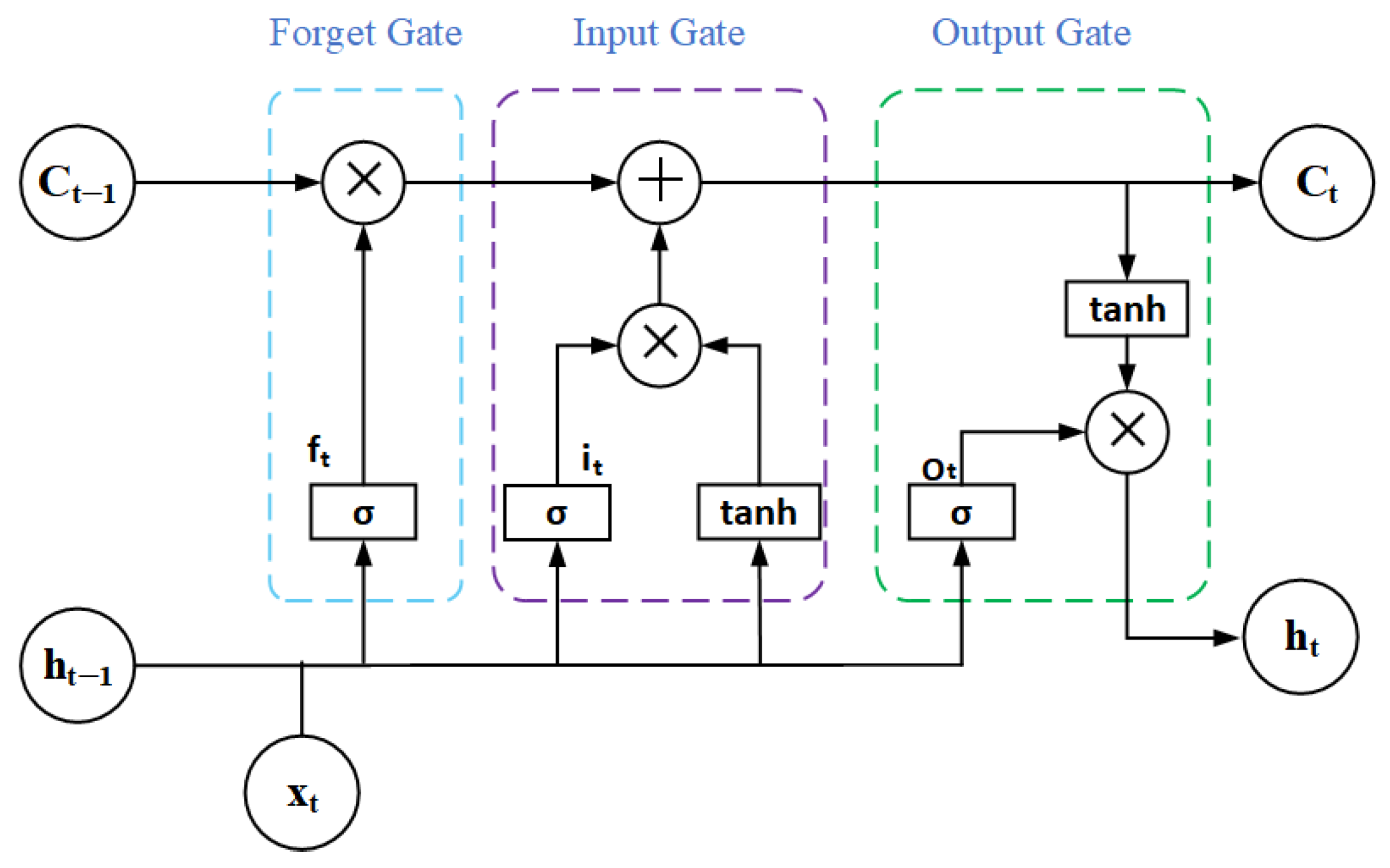
Although existing methods have made valuable progress in predicting oil temperature using deep learning methods, there are still many limitations: (1) Most current methods use small-scale experimental datasets, typically focusing on a single transformer with just hundreds of data groups, and often idealized data. However, in real-world engineering applications, datasets are usually larger and more complex [17]. Raw data is often hard to use directly for model training. This results in the poor generalization of existing research models, making them ill-suited for practical engineering scenarios. (2) In practical engineering applications, raw data needs to be analyzed and preprocessed to fit the model’s input criteria. As the data sampling duration increases, the influence of external factors, like ambient temperature, on the model becomes substantial and must not be overlooked [18]. 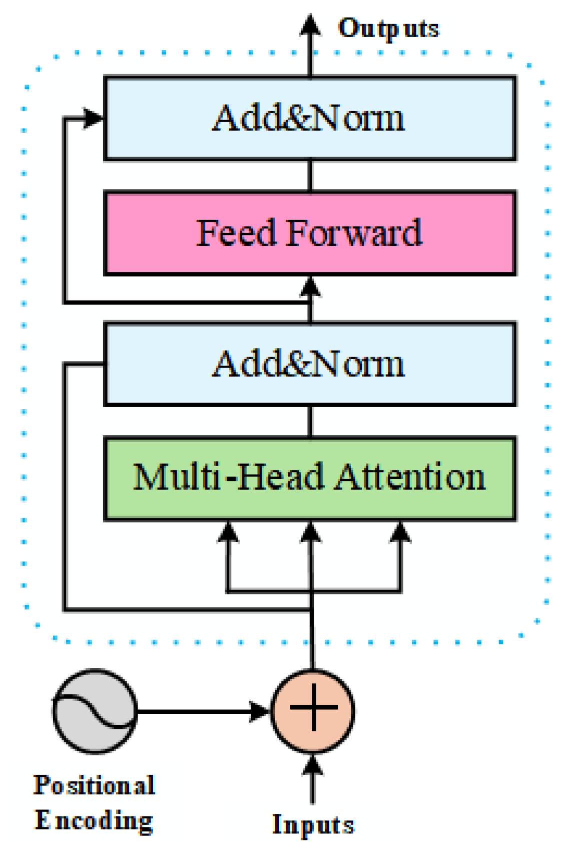Conventional models often struggle to effectively learn the complex coupling relationships between historical oil temperature data and other influencing factors, which further limits the model’s performance in real-world applications [19]. To address these challenges, this paper proposes a forecasting method for transformer oil temperature time-series data based on a hybrid architecture of a CNN-LSTM-Transformer. Aiming to boost the model’s generalization ability, this method includes a thorough analysis and preprocessing of transformers’ actual operation data. First, duplicate data is removed, missing data is reasonably imputed, and abnormal data is identified and eliminated. The process of identifying abnormal data integrates outlier detection theory with practical operation and maintenance experience. In addition, by calculating the correlation coefficients between transformer oil temperature and each characteristic variable, key factors that significantly affect oil temperature changes are selected, thereby comprehensively considering the combined effect of various transformer characteristics on oil temperature. Leveraging time-sequence data that includes transformer oil temperature and various associated features as input, this research introduces a prediction approach grounded in a combined CNN-LSTM-Transformer framework. The method first employs CNNs to extract spatial features from multiple input features and explore feature relationships. Subsequently, LSTM networks are utilized to discern the temporal variations in the time-sequence data and further extract temporal features. Finally, a Transformer encoder is integrated to enhance feature interaction and global perception capabilities. This approach integrates the spatial characteristics obtained via CNN and the temporal characteristics obtained via LSTM to produce a more comprehensive feature representation, which leads to more accurate and generalized prediction outcomes. The experimental findings show that the proposed model surpasses existing models in terms of prediction accuracy. The established model was optimized using the WOA to improve prediction accuracy. Compared with the most advanced methods, the proposed method is novel in the following aspects:

• Innovative Model Architecture: This study proposes a novel hybrid model architecture that integrates the CNN, LSTM, and Transformer encoder for predicting transformer top oil temperature. This combination leverages the strengths of each component to effectively capture both spatial and temporal features from the input data, providing a more comprehensive and accurate representation for prediction.
• Enhanced Generalization Capability: This method incorporates thorough data analysis and preprocessing techniques, including data cleaning, normalization, and feature selection based on correlation coefficients. This ensures the model can handle large-scale, complex datasets with various influencing factors, significantly improving its generalization ability for practical engineering applications.
• Improved Prediction Accuracy: The proposed model achieves superior prediction accuracy compared to existing methods, as demonstrated by the experimental results. The maximum RMSE and MAPE of this method on the summer and winter datasets are 0.5884 and 0.79%, respectively, indicating its high precision and reliability in forecasting transformer top oil temperature.
• Practical Engineering Application: This research provides a practical and effective solution for transformer condition monitoring and fault warning in power systems. By accurately predicting the top oil temperature, it helps optimize maintenance strategies, enhance the reliability of power systems, and extend the lifespan of transformers, contributing to the efficient and safe operation of power equipment.

Table 1. Comparison of model innovation.

Model Variant	Model Comparison
Random Forest [10]	Significant disadvantages in high-precision time series prediction tasks
CNN-LSTM [20,21]	Lack of global awareness
CNNs-Transformer [22]	Insufficient capture of time dynamics patterns
LSTM-Attention [23]	Ignoring spatial characteristics
Proposed Model	Combining the advantages of various components to achieve spatiotemporal feature fusion

lists the innovative features of the model architecture in this paper and compares it with other hybrid models in the literature, highlighting the theoretical advantages of the model in this paper and emphasizing its uniqueness.

The results of the experiment indicate that the maximum RMSE and MAPE of this method on the summer and winter datasets are 0.5884 and 0.79%, respectively, demonstrating superior prediction accuracy. Compared with other models, the proposed model improved prediction performance by 13.74%, 36.66%, and 43.36%, respectively, indicating high generalization capability and accuracy. This provides theoretical support for condition monitoring and fault warning of power equipment.

2. Model Construction

2.1. CNN

CNNs are a type of deep learning architecture widely used in image recognition, speech processing, time-series analysis, and more [24]. Their key strength lies in automatically extracting local features from data and capturing complex patterns through a hierarchical structure. Relative to traditional machine learning methods, CNNs excel in feature extraction. They can automatically learn optimal feature representations from data, reducing the reliance on manual feature extraction and able to effectively extract spatial features from large-scale transformer data. This capability has been effectively leveraged in power system research and analysis, where CNNs have demonstrated superior performance [20,21,22].

2.2. LSTM Neural Networks

LSTM is a particular kind of Recurrent Neural Network that targets the vanishing and exploding gradient challenges faced by traditional RNNs in long-sequence processing. By introducing a “gating mechanism” and a “cell state” [23,25,26,27,28], LSTM can effectively capture long-term dependencies in large-scale transformer data sequences. The fundamental unit structure of an LSTM network is depicted in Figure 1.

2.3. Transformer Encoder

The Transformer is a deep learning system based on self-attention mechanisms. Its core idea is to process all elements in a sequence in parallel using self-attention, relying entirely on attention mechanisms to capture long-range dependencies. This significantly improves training speed and model performance [29,30,31,32,33]. In this study, the proposed model primarily leverages the powerful capabilities of the Transformer encoder to enhance the predictive performance of transformer oil temperature time series data. The Transformer encoder, through its unique self-attention mechanism, enables the model to capture long-range dependencies in sequence data, which is particularly important for handling time series data from power systems with complex dynamic characteristics. The structure of the Encoder is shown in Figure 2.

2.4. WOA

As a meta-heuristic optimization algorithm, the Whale Optimization Algorithm simulates the bubble-net hunting behavior of humpback whales. The core of this algorithm lies in simulating three main hunting behaviors of humpback whales: encircling prey, spiral movement, and searching for prey [21,34,35,36]. In the search space, individuals of the WOA are centered around the current optimal solution and update their positions in various ways to approach and search for the optimal solution. During each round of iteration, the algorithm determines which update method to use based on a uniformly distributed probability $p\in [0,1]$.

When the condition $p\ge 0.5$ is met, the spiral-like update process is activated, causing individuals to spiral towards the prey. The position update is depicted in the following formula (Formula (1)):

$$\stackrel{\rightharpoonup }{X}(t+1)=\stackrel{\rightharpoonup }{D}\cdot e^{b\cdot l}\cdot \cos (2\pi l)+{\stackrel{\rightharpoonup }{X}}^{\ast }(t)$$

(1)

where ${\stackrel{\rightharpoonup }{X}}^{\ast }(t)$ denotes the location of the best whale in the current population, $\stackrel{\rightharpoonup }{D}=\left|{\stackrel{\rightharpoonup }{X}}^{\ast }(t)-\stackrel{\rightharpoonup }{X}(t)\right|$ indicates the gap between the whale and the prey, b is the constant defining the spiral shape, and $l\in [0,1]$ is a randomly generated value used to simulate the nonlinear approach path.

When p < 0.5 is satisfied, the algorithm decides to perform either contraction encircling or global searching based on $\left|\stackrel{\rightharpoonup }{A}\right|$. When $\left|\stackrel{\rightharpoonup }{A}\right|<1$ is satisfied, it performs local searching, which means contraction encircling the prey:

$$\stackrel{\rightharpoonup }{X}(t+1)={\stackrel{\rightharpoonup }{X}}^{\ast }(t)-\stackrel{\rightharpoonup }{A}\cdot \left|\stackrel{\rightharpoonup }{C}\cdot {\stackrel{\rightharpoonup }{X}}^{\ast }(t)-\stackrel{\rightharpoonup }{X}(t)\right|$$

(2)

$$\stackrel{\rightharpoonup }{A}=2\stackrel{\rightharpoonup }{a}\cdot {\stackrel{\rightharpoonup }{r}}_1-\stackrel{\rightharpoonup }{a}$$

(3)

$$\stackrel{\rightharpoonup }{C}=2\cdot {\stackrel{\rightharpoonup }{r}}_2$$

(4)

where $\stackrel{\rightharpoonup }{a}$ reduces linearly from 2 to 0 with the growing number of iterations, and $r_1,r_2\in [0,1]$ are two independent random vectors. When $\left|\stackrel{\rightharpoonup }{A}\right|\ge 1$, the algorithm then enters the search for prey phase, randomly selecting individuals ${\stackrel{\rightharpoonup }{X}}_{rand}$ from the population and updating the formula:

$$\stackrel{\rightharpoonup }{X}(t+1)={\stackrel{\rightharpoonup }{X}}_{rand}-\stackrel{\rightharpoonup }{A}\cdot \left|\stackrel{\rightharpoonup }{C}\cdot {\stackrel{\rightharpoonup }{X}}_{rand}-\stackrel{\rightharpoonup }{X}(t)\right|$$

(5)

The WOA is widely used in function optimization, feature selection, hyperparameter tuning of deep learning models, etc., due to its simple structure, strong global search ability, and fast convergence speed. In this study, the WOA is applied to automatically optimize several key hyperparameters of the LSTM layer, covering the count of layers, the count of units, the count of Transformer heads, and the learning rate. By defining the prediction error (Mean Squared Error, MSE) on the validation set as the fitness function, the algorithm guides the population to iteratively evolve toward better hyperparameter combinations, thereby enhancing the overall predictive performance of the model. The flowchart for optimizing hyperparameters in this paper is as follows Figure 3:

2.5. CNN-LSTM-Transformer

Figure 4 depicts the prediction workflow suggested in this paper, which is based on the CNN-LSTM-Transformer hybrid model. This model integrates Convolutional Neural Networks (CNNs), Long Short-Term Memory (LSTM) networks, and Transformer encoders, leveraging the advantages of each component through a multi-model combination approach to achieve more accurate prediction results. The CNN layer is responsible for extracting spatial features from multi-dimensional input features. Through convolution operations, the CNN can capture local patterns and feature relationships in the input data. The LSTM layer is used to capture dynamic changes in time-series data. The spatial features extracted by the CNN layer and the temporal features extracted by the LSTM layer are integrated to form a more comprehensive feature representation. This integration enables the model to consider features across both spatial and temporal dimensions, thereby achieving more accurate predictions of transformer top oil temperature. The Transformer encoder further enhances the model’s ability to perceive global features through self-attention mechanisms. Through the self-attention mechanism, the model can better capture complex relationships and long-term dependencies between features. This synergistic interaction among multiple components significantly improves the model’s prediction accuracy and generalization ability.

To better capture the time-series features, data sliced via a sliding window approach is utilized for forecasting future transformer oil temperatures. Initially, in the first step of input sequence data handling, the initial dataset is converted into high-dimensional sequence data as input in the form of fixed-size vectors. The raw dataset consists of a time series denoted as $[X_1,X_2,X_3,\text{...},X_n]$. A series of sequences X is created as a time window data with a fixed T length $[X_1,X_2,\text{...},X_n]$, where $X_t$ consists of $[x_1,x_2,\text{...},x_m]$, representing m feature inputs at each time step. The length of the sliding window is decided according to the number of prediction time steps. This step reshapes one-dimensional sequential data into a two-dimensional tensor as input data, where one dimension contains t time steps and the other dimension contains the features. For example, four features were selected, and the time steps were set to 40 (representing 40 min intervals), resulting in an input shape of 40 × 4. During training, samples were processed in batches, with a batch size of 64, resulting in an input tensor size of 64 × 40 × 4. Subsequently, the processed data was fed into a 1D convolutional layer. The input sequences are processed through two 1D convolutional layers to capture local temporal features. The convolution operation effectively identifies short-term trends and local patterns in the data. Additionally, dimensionality reduction was performed using max-pooling operations. Prior to entering the 1D convolutional network module, the input tensor was transposed from 40 × 4 to 4 × 40 to match the input format of the Conv1D layer. Finally, the data sequentially passed through two convolutional layers and two max-pooling layers:

$$Y_{CNN}=CNN(X;{\theta }_{CNN})$$

(6)

where $X\in R^{T\times d}$ represents the input time series, T indicates the count of time steps (fixed at 40), and d represents the feature dimension at each time step (set to 4). Y represents the output from the CNN layer, and $\theta$ represents all parameters of the CNN layer. The first convolutional layer expands the number of channels from 4 to 64 while preserving the sequence length. After pooling, the sequence length is reduced to 20. The second convolutional layer further expands the number of channels from 64 to 128, and after another pooling operation, the sequence length is further reduced to 10. At this point, the output tensor has a shape of 128 × 10. Subsequently, the temporal data extracted by the CNN is transposed to 10 × 128 and fed into a multi-layer LSTM. The LSTM is utilized to reveal enduring relationships in the historical oil temperature data and can grasp enduring relationships and intricate temporal dynamics within the data. In the constructed model, each LSTM layer consists of ten LSTM units, each processing samples from a single time step. These LSTM units collaborate sequentially. The initial LSTM unit handles the input sample and conveys the processed data to the subsequent LSTM unit. The subsequent LSTM unit then assesses whether to preserve the data received from the initial unit. If it decides to retain this information, it retains it in the enduring memory module and conveys both the processed data from the first unit and the current sample’s feature information to the third LSTM unit. This process continues sequentially until the last LSTM unit, which ultimately integrates all the processed information from the previous LSTM units:

$$h_t,c_t=LSTM(Y_{CNN},h_{t-1},c_{t-1};{\theta }_{LSTM})$$

(7)

Assuming the LSTM adopts a two-layer structure, the count of hidden units in the LSTM is set to 64. As a result, the output tensor size of the LSTM units is 10 × 64, consisting of ten sets of 1 × 64 data. Building on this, the output is further fed into the Transformer encoder to fully model the global dependencies between different time steps. The Transformer’s self-attention mechanism allows the model to concentrate on the correlations between any two time points in the input sequence, effectively identifying the underlying global patterns and long-range dependencies in the oil temperature time series. The Transformer keeps its input and output shapes consistent, resulting in ten sets of 1 × 64 tensor data:

$$Y=Transformer(h_t;{\theta }_{Transformer})$$

(8)

where $Y$ is a further processing of sequence information through a multi-head attention mechanism and a feed-forward neural network. The model extracts the representation of the last time step (i.e., step 10) from the output of the Transformer to obtain a tensor of dimension 1 × 64. This tensor is passed through a fully connected layer that reduces the feature dimensions to 1 for the final prediction. The pseudocode for this model is as follows Algorithm 1:

Algorithm 1: WOA-Optimized CNN-LSTM-Transformer Model

Input: raw input data: Oil Temperature, Current Load Current, Load Ratio, Ambient Temperature;

Hyperparameters: maximum iterations I = 30, population size N = 20, spiral coefficient b = 1, convergence factor a = 2, LSTM layers range [1, 4], LSTM units range [64, 256], Transformer heads range [1, 4], learning rate range [0.01, 0.0001];

Initialize: whale population W = [w1, w2, …, w, N], best whale = None, best fitness = −infinity;

normalize input data;

for each whale w in W do    cnn features = CNN(w. cnn_params, input_data);    lstm output = LSTM(w. lstm_params, cnn_features);    transformer output = Transformer(w.trans_params, lstm_output); end

predicted_oil_temp = DenseLayer(transformer_output);

for each whale w in W do    fitness = evaluate_fitness(w, actual_oil_temp, predicted_oil_temp);    if fitness > best_fitness then    best_fitness = fitness;    best_whale = w; end end

for t = 1 to I do    for each whale w in W do       update_position(w, best_whale, t, I);    end       update best_whale and best_fitness; end

Return: predicted oil temperature using best_whale parameters;

3. Experimental Design and Result Analysis

In this paper, the experimental hardware environment consists of an NVIDIA GeForce GTX 1660 Ti GPU and 6 GB of RAM, and experiments are conducted in Windows 10 using Python 3.9 language and the PyTorch 2.2.2 framework for neural network model building. With the primary objective of predicting transformer top oil temperature, in order to enhance the prediction accuracy and prediction generalization, the data must be analyzed and processed as a priority, and the data processing specifically comprises data categorization, feature extraction, data purification, data normalization, and data slicing and dicing.

3.1. Data Preprocessing

To construct an accurate top oil temperature prediction model for transformers, this study collected live monitoring data from several substations in a specific region over a twelve-month period from May 2023 to April 2024. Environmental temperature data were supplemented by querying relevant meteorological records, ensuring consistency in the timestamps of all datasets. The schematic diagram of the transformer equipment and oil temperature sensor is shown in Figure 5.

The specific data collected include key parameters such as the transformer’s current load, environmental temperature, top oil temperature, and load current, as shown in

Table 2. Type of data.

Number	Category	Unit
1	Oil Temperature	°C
2	Current Load Current	A
3	Phase A/B/C Current	A
4	Active Power	W
5	Reactive Power	W
6	Load Ratio
7	Maximum Load of the Day	A
8	Average Load Ratio
9	Ambient Temperature	°C

.

Recorded with a sampling period of every minute, the overall size of the data is about 9 million groups. The collected dataset is notable for its large volume, diverse types, and the representation of actual operating conditions of various transformers across different time periods and seasons. This enables the transformer prediction model to effectively identify and interpret the intricate relationships within the data, thereby enhancing the model’s generalization capability. A glimpse of the data’s actual situation is presented in

Table 3. Part of the real data.

ID	Time	Oil Temperature (°C)	Load Ratio	Ambient Temperature (°C)	Load Current (A)	Active Power (W)	Reactive Power (W)
14	1 January 2024 00:06:00	31.0476	35.9124	12.733	17.9562	90.5842	9.7746
15	1 January 2024 00:06:00	30.6812	35.1837	12.733	17.7470	91.5628	11.7512
16	1 January 2024 00:06:00	30.9743	34.2476	12.469	17.1584	73.4511	0
17	1 January 2024 00:06:00	1.83 × 10−32	33.9267	12.469	16.8655	89.9314	8.6482
18	1 January 2024 00:06:00	30.9011	33.3023	12.874	16.8681	93.5796	9.2585
19	1 January 2024 00:06:00	30.8735	34.4594	12.7622	16.9521	91.5731	9.5781
20	1 January 2024 00:06:00	31.0187	34.4799	12.4872	17.1467	93.7821	10.4722

.

From Table 2, in part of the real data situation, the following can be seen: the real data in the characteristics of many categories, the need to carry out the selection of features, a greater correlation between the characteristics of the selected oil temperature change, the existence of different transformer models, the cooling mode, the rated capacity, and different operating voltages. In addition, it can be seen that the time points of different equipment data are together. If you want to subsequently classify the operation of the transformer, data processing is necessary and different equipment transformer data must be extracted separately to obtain the time series data of each transformer, to enable the subsequent integration of transformers of the same type. In addition, from the 12-month raw data obtained, it is found that there are differences in the data scale of different months, which is usually caused by substation maintenance or data transmission process loss, and from the table, it can also be observed that there are evident anomalous data and missing values; for example, in the oil temperature of transformer no. 17, the transformer data of 1.83 × 10⁻³² is obviously anomalous, and in the third data point, the reactive power appears to have a value of zero. If these abnormal data points are directly fed into a model, it will impact the model’s robustness and forecasting capability. Hence, the raw data requires processing. The data processing procedure is depicted in Figure 6:

3.1.1. Data Classification

Data categorization is divided into two main steps, the categorization of individual transformers and the categorization of transformer types. In the raw dataset, the data of different transformer devices at a point in time are mixed together, so the raw dataset needs to be classified according to the data of different numbered transformers in order to extract the continuous and independent time-series data of each transformer over a twelve-month period.

After obtaining the sequential data of each transformer, the required data need to be extracted according to the task requirements to reduce the workload. The majority of current studies concentrate solely on predicting data for a single transformer, and this research method has limitations in enhancing the model’s adaptability, making it hard to satisfy the actual engineering needs. In addition, considering the diverse range of equipment types and models of transformers, significant disparities exist in the change patterns of actual operating data and their potential characteristic relationships for different categories of transformers. Although some research tries to use the transformer category directly as input features for the model, with the ongoing increase in prediction accuracy requirements, the effectiveness of this method has struggled to meet current practical prediction demands.

To address the aforementioned issues, this paper puts forward an improvement strategy: first, the type of transformer is categorized and, in the collected data, can be used as the basis for classifying transformer category information. There are different types of transformers, rated capacities, and operating voltages. Through existing research, it has been observed that the temperature rise of transformers varies significantly with different operating voltages, so classification depends on the operating voltage and the cooling mode of the transformer [37]. After categorization, the operating voltage of the obtained transformer data is divided into two classes: 110 kV and 220 kV. The cooling methods include three types: oil-immersed self-cooled (ONAN), oil-immersed air-cooled (ONAF), and forced oil-circulation air-cooled (ODAF) systems. Subsequently, random sampling is conducted among transformers of the same category. For instance, data from five transformers are randomly selected for model training, and then data from new transformers (other than the aforementioned five) within the same category are randomly extracted for prediction, to validate the model’s generalization ability. This study selects 110 kV transformers with an ONAN cooling method as the research subjects. Seven transformers of this category are randomly selected as experimental data, and subsequent data processing operations are also based on this dataset.

3.1.2. Feature Selection

After data classification is completed, feature selection is performed. The collected transformer data contains a large number of features, but not all of them are primary correlated features with oil temperature. Accurately identifying features closely related to oil temperature is crucial for improving prediction accuracy. Therefore, the Pearson correlation coefficient (PCC) [38,39,40] and mutual information (MI) are used to select primary features. The PCC is used to assess the linear relationship between candidate features and oil temperature, while MI is used to assess nonlinear relationships for feature selection. The specific calculation formulas are as follows:

$$r_{xy}={\displaystyle \frac{{\displaystyle \sum (x_i-\overline{x})(y_i-\overline{y})}}{\sqrt{{\displaystyle \sum {(x_i-\overline{x})}^2{\displaystyle \sum {(y_i-\overline{y})}^2}}}}}$$

(9)

where $x_i$ and $y_i$ denote the feature value and oil temperature, respectively, and $\overline{x}$ and $\overline{y}$ are the respective mean values. If $\left|r_{xy}\right|$ is closer to 1, it means that the feature is more closely related to the oil temperature, which can be used as the key variable; if r is closer to 0, it means that the correlation is weak and can be removed.

When calculating mutual information, the continuous input features are first discretized using an equal-frequency discretization method, dividing each feature into 10 intervals such that the number of data points within each interval is approximately equal. This method effectively avoids issues caused by uneven data distribution, such as certain intervals having overly dense or sparse data, thereby ensuring more stable and accurate mutual information calculations. After completing the data discretization, a histogram-based method is used to estimate the probability distribution. For each feature X and target variable Y, the number of data points in each interval is counted. For example, for the i-th interval of X and the j-th interval of Y, the number of data points N_ij that fall into both intervals is counted. The joint probability $p(x_i,y_i)$ can then be estimated as ${\displaystyle \frac{N_{ij}}{N}}$, the marginal probabilities $p(x_i)$ and $p(y_j)$ can be estimated as ${\displaystyle \frac{{\displaystyle {\sum }_{j=1}^n{N}_{ij}}}{N}}$ and ${\displaystyle \frac{{\displaystyle {\sum }_{i=1}^m{N}_{ij}}}{N}}$, respectively, and finally, mutual information is calculated using Formula (10).

$$I(X;Y)={\displaystyle {\sum }_{i=1}^m{\displaystyle {\sum }_{j=1}^{n}p(x_i,y_j)}}\log ({\displaystyle \frac{p(x_i,y_j)}{p(x_i)p(y_j)}})$$

(10)

where m and n represent the number of intervals for features X and Y, respectively, and N represents the total number of data points. The higher the mutual information value, the stronger the dependence between the feature and the oil temperature.

This study selected features with a significant correlation with oil temperature changes. The PCC and MI values between each feature and oil temperature are shown in

Table 4. Results of feature correlation.

Category	PCC	MI
Load Ratio	0.6783	0.45
Ambient Temperature	0.6854	0.42
Current Load Current	0.7532	0.50
Current Phase C	0.2954	0.15
Current Phase C	0.3458	0.18
Current Phase C	0.3156	0.16
Active Power	0.5428	0.30
Reactive Power	0.2677	0.12

. The table indicates that the PCC and MI values for phase current, active power, and reactive power are relatively low, suggesting that these features have weak linear and nonlinear relationships with oil temperature and can be removed. However, the PCC and MI values between the ambient temperature, load factor, current load current, and transformer oil temperature are relatively high, indicating that these features have a significant correlation with oil temperature and can be used as key features. Therefore, based on historical oil temperature data, the ambient temperature, load factor, and current load current are also added as input features.

3.1.3. Dataset Partitioning

In order to verify the feasibility of the combined model approach in the case of real complex data, and to improve the generalization of the prediction, the five units in the previous section are randomly selected. In the training phase of the model, 2,628,000 datasets of 110 kV and ONAN transformer types numbered 1, 14, 54, 68, and 257 were utilized for a one-year period, and these datasets were divided into training and validation sets in a ratio of 8:2. In selecting the test set, the influence of the season on model prediction results is considered. Two groups of experimental test datasets were constructed in summer and winter, of which transformer no. 79 was randomly selected for the winter one, 21 January 2024–31 January 2024, representing a total of 14,400 groups of data, and transformer no. 49 was randomly selected for the summer one, 1 August 2023–10 August 2023, representing a total of 14,400 groups of data.

3.1.4. Data Cleaning

The data cleaning work mainly involves filling in missing values and filtering out outliers. In the initial data checking stage, the problem of missing values and outliers is evident in some features through observation and analysis. The presence of missing values interferes with the training and prediction performance of the model, and outliers are data points that markedly diverge from the normal range, usually resulting from sensor failures or data acquisition errors.

In this paper, the theoretical method and the real-world operation and inspection guidelines are used to monitor and process the outliers. The theoretical method employs an LSTM autoencoder-based anomaly detection technique [41], which detects outliers in time-series data by computing the discrepancy between the reconstructed and original transformer oil temperature values and contrasting it with a predetermined threshold. The operation and inspection rules are derived from the transformer’s operational and maintenance experience and its operational behavior. For instance, during normal transformer operation, oil temperature data surpassing the 90-degree threshold is deemed abnormal, oil temperature data that continuously jumps by more than 1 degree is seen as abnormal, and load ratio data that continuously jumps by more than 100% is also viewed as abnormal, among others. Integrating both theoretical approaches and practical operation and inspection rules can more precisely identify transformer data outliers and enhance the standardization and precision of the dataset [42]. Figure 7 shows the data before and after cleaning. During the data cleaning process, a total of 45,705 outliers were detected and removed, accounting for 1.74% of the total data volume. The removal of these outliers significantly improved data quality and model robustness. Additionally, the study found that there were 3218 missing values in the original data, accounting for 0.12% of the total data volume. We used mean imputation to fill in the missing values, ensuring the completeness and consistency of the data.

3.1.5. Data Normalization

Considering the notable differences in the magnitude and value range of various features, the direct use of raw data may lead to numerical instability during model training. Therefore, all features are normalized and scaled within the range of [0, 1]. The formula for normalization is presented below:

$$x^{\prime }={\displaystyle \frac{x=x_{\min }}{x_{\max }-x_{\min }}}$$

(11)

where x stands for the original feature value and x’ is the normalized feature value, where $x_{\max }$ and $x_{\min }$ are the maximum and minimum values of the original feature value, respectively. The normalization process not only boosts the model’s training efficiency but also heightens its sensitivity to different features, which helps improve prediction accuracy.

3.1.6. Time-Window-Based Data Segmentation

Transformer oil temperature data exhibits distinct time-series characteristics. Thus, in the data preprocessing stage, the impact of the time factor must be fully considered. For the standardized oil temperature and transformer characteristics data, cutting is performed according to a time window. For instance, a time window size of x means the data is divided into segments every x minutes. Starting from the first time step of the dataset, each window encompasses data from x consecutive time steps. Then, the window is gradually slid forward. This approach ensures that the generated data batches retain the continuity of the time-series, facilitating model training and allowing the capture of data characteristics over time [43].

3.2. Evaluation Metrics

To comprehensively evaluate how well the proposed model predicts oil temperature, the model’s performance is assessed using MAPE, MAE, RMSE, and R², which are common metrics for evaluating prediction accuracy.

$$MAPE={\displaystyle \frac{1}{n}}{\displaystyle \sum _{i=1}^n\left|\frac{y_{true}-y_{pre}}{y_{true}}\right|}\times 100\%$$

(12)

$$MAE={\displaystyle \frac{1}{n}}{\displaystyle \sum _{i=1}^n\left|y_{true}-y_{pre}\right|}$$

(13)

$$RMSE=\sqrt{{\displaystyle \frac{1}{n}}{{\displaystyle \sum _{i=1}^n(y_{true}-y_{pre})}}^2}$$

(14)

$$R^2=1-{\displaystyle \frac{{\displaystyle {\sum }_{i=1}^n{(y_{true}-y_{pre})}^2}}{{\displaystyle {\sum }_{i=1}^n{(y_{true}-\overline{y})}^2}}}$$

(15)

where $y_{true}$ denotes the actual value; $y_{pre}$ represents the model’s predicted value; $\overline{y}$ indicates the mean of the actual values; and n stands for the sample count. Lower MAPE, MSE, and RMSE values signify better performance. The value of R² is in the range of (−∞, 1], and the closer it is to 1, the better the effect, which means that the model’s prediction accuracy is higher. In the analysis of the experimental results, this paper compares the performance advantages and disadvantages of different model structures and parameter settings based on the above four indicators, in order to verify the effectiveness and generalization ability of the proposed method.

3.3. Parameter Selection

In this study, the CNN uses a two-layer 1D Convolutional Neural Network. The convolutional kernel is set to 3. The first layer has 64 channels and the second layer has 128 channels. The pooling layer employs a maximum pooling operation, with both the size and stride set to 2. The batch size is 64. To boost the model’s performance in oil temperature prediction, the WOA automatically optimizes key hyperparameters. Initially, the primary parameters of the WOA are configured as follows: the population size is set to 20 and the maximum number of iterations is 30; the spiral coefficient b is 1; and the contraction factor a is 2. The quantity of LSTM layers fluctuates from 1 to 4, and the units in each LSTM layer span from 64 to 256. For the Transformer, the number of attention heads is between 1 and 4, and the learning rate ranges from 0.0001 to 0.01.

After iterative computation, the number of LSTM layers is obtained as 2, the LSTM layer has 64 cells, the Transformer layer has 2 attention heads, and the learning rate is 0.001.

3.4. Ablation Experiment

To investigate the contribution of each model component to prediction performance, this study designed a series of ablation experiments. Ablation experiments selectively remove or modify certain parts of the model to observe the impact of these changes on model performance, thereby assessing the importance of each component. The ablation experiments in this study primarily focus on the CNN-LSTM-Transformer model, aiming to validate the roles of the CNN layer, LSTM layer, and Transformer layer in the task of predicting the top-layer oil temperature of a transformer. The proposed model is the complete CNN-LSTM-Transformer model, whose structure and parameter configuration are as described earlier. In the ablation experiments, the following model variants were evaluated: Model 1 removes the CNN layer, retaining only the LSTM and Transformer layers; Model 2 removes the LSTM layer, retaining only the CNN and Transformer layers; Model 3 removes the Transformer layer, retaining only the CNN and LSTM layers; and Model 4 replaces the LSTM layer with a standard RNN layer, with the remainder unchanged. The test sample is the summer data of transformer no. 49. All models were trained and evaluated on the same training and validation datasets to ensure the comparability of experimental results, as shown in

Table 5. Ablation experimental results.

Model Variant	MAPE (%)	MAE (°C)	RMSE (°C)	R2
Model 1	0.8754	0.5122	0.7041	0.9869
Model 2	1.5124	0.8461	1.0842	0.9739
Model 3	1.2782	0.643	0.9262	0.9802
Model 4	2.5298	1.3453	1.8473	0.9629
Proposed Model	0.6048	0.2924	0.4255	0.9974

:

As shown in Table 4, the proposed model performs best across all evaluation metrics, indicating that the combination of CNN layers, LSTM layers, and Transformer layers is crucial for accurately predicting the top-layer oil temperature of transformers. Removing any component results in a decline in model performance, with Model 2 showing the most significant impact when the LSTM layer is removed, resulting in an increase of 0.6587 in RMSE and a decrease of 0.0235 in R². This indicates that the LSTM layer plays a crucial role in capturing long-term dependencies in time series data. Additionally, replacing the LSTM layer with a standard RNN layer in Model 4 also leads to a noticeable decline in performance, further validating the advantages of the LSTM layer. Through ablation experiments, this study validated the effectiveness of each component in the CNN-LSTM-Transformer model. The experimental results show that the CNN layer, LSTM layer, and Transformer layer all play important roles in predicting the top oil temperature of transformers and are indispensable. The organic combination of these components enables the model to predict the top oil temperature of transformers more accurately, providing strong support for the condition monitoring and fault warning of power equipment.

The second ablation experiment was conducted to validate the performance of the WOA in optimizing model hyperparameters. The search space for hyperparameter optimization in transformer oil temperature prediction is highly complex, involving multiple dimensions (e.g., LSTM layers, units, Transformer heads, learning rate) and nonlinear relationships. The WOA’s unique mechanisms—such as encircling prey, spiral movement, and random search—enable it to balance global exploration and local exploitation effectively. Unlike Bayesian optimization, which relies on prior assumptions (e.g., Gaussian processes) and may struggle with high-dimensional or non-convex spaces, the WOA adapts dynamically to the search landscape. Furthermore, while random search lacks guided exploration and often converges slowly, the WOA’s mimetic whale behavior allows it to efficiently locate optimal hyperparameter combinations, even in complex scenarios. Therefore, we performed a comparative experiment using the WOA, Bayesian optimization, and random search to optimize the model. Bayesian optimization used a Gaussian process sampling method with 50 sampling points, while random search had 10 sampling points. The convergence criterion was set to 10 consecutive iterations with no significant changes in the objective value. The parameter search range for random search was the same as that for the WOA, and the seed was fixed at 42 to ensure reproducibility of the results. The experimental results showed that the WOA outperformed the other methods in terms of optimization performance. The specific results are shown in the

Table 6. Comparison of optimized algorithm results.

Optimization Method	MAPE (%)	Maximum RMSE (°C)
WOA	0.7892	0.5521
Bayesian optimization	0.8461	0.6133
Random search	0.9234	0.6789

below:

As can be seen from Table 5, the WOA performs best in terms of optimization performance, with both maximum RMSE and MAPE lower than those of other methods. This indicates that the WOA has a significant advantage in optimizing the hyperparameters of complex models. In addition to achieving a lower MAPE and RMSE, the WOA demonstrates superior performance in terms of convergence speed and computational efficiency. As shown in the figure of the number of iterations during training in Figure 8, the WOA converges within 30 iterations, while Bayesian optimization requires more sampling points (approximately 50) to achieve a similar effect, and random search cannot converge sufficiently within the same number of iterations. This fully demonstrates the WOA’s ability to search more efficiently in complex search spaces, making it particularly suitable for optimizing deep learning models in practical engineering applications.

3.5. Analysis of Prediction Results

The forecasting technique for transformer oil temperature time series data based on the CNN-LSTM-Transformer combination model is used to model and predict the randomly selected non-training set of the summer sample data of transformer no. 49 and the winter sample data of transformer no. 79, respectively, and to analyze the prediction method on different cases of datasets.

Table 7. Experimental results.

Dataset	MAPE/%	MAE/°C	RMSE/°C	R2
Summer Data	0.4678	0.2339	0.4053	0.9985
Winter Data	0.7992	0.3996	0.5884	0.9862

presents the error statistics for the two test samples. As indicated by the data in the table, the combination model method based on the CNN-LSTM-Transformer demonstrates a more favorable performance when dealing with large-scale datasets. The MAE between the test values and the actual values is maintained below 0.5 percent, which adequately reflects the accuracy and generalization ability of the method introduced in this paper.

Figure 9 and Figure 10 display the comparative graphs of forecasted and actual oil temperatures for transformers numbered 49 and 79. As shown in the figures, the forecasted oil temperature values show a high level of precision. Although there is a slight error in predicting the peak values, with deviations of approximately 1 degree, the general course of the predicted values closely coincides with that of the actual values. Additionally, a visual analysis of the uncertainty in the model’s prediction results was conducted by plotting the 95% confidence intervals of the predicted values to intuitively demonstrate the reliability and fluctuation range of the prediction results. When plotting the comparison chart between predicted and actual values, in addition to separately displaying the actual values (blue solid line) and predicted values (red solid line), two additional gray dashed lines were plotted to represent the upper and lower bounds of the 95% confidence interval. This interval to some extent reflects the statistical uncertainty of the model’s predicted results; the higher the proportion of actual values falling within this interval, the higher the accuracy of the model’s predictions. As shown in the figure, the actual values are mostly within the confidence interval, demonstrating the robustness of the model in this paper. This provides a more comprehensive and reliable reference for decision making based on model predictions in practical applications.

To visually demonstrate the error between the model’s predicted values and actual values, we plotted a residual line chart. Figure 11 shows the residual line chart of the prediction model in this paper, which captures 1440 time points within a single day on 1 August 2023. As can be seen from the figure, most of the errors are concentrated around zero, indicating that the model has high predictive accuracy, with the predicted results being very close to the actual values. Although there are some points with larger errors, these points account for a small proportion of the entire dataset, and the prediction errors are all stable below 0.5 degrees Celsius, demonstrating the model’s robustness and reliability.

3.6. Comparison Experiment

To further verify the prediction accuracy of the CNN-LSTM-Transformer model in the task of oil temperature prediction, this paper compares its performance with multiple classical prediction methods under the same dataset and feature conditions, respectively. The selected prediction methods are Informer, TCN, and LSTM-Attention methods; all models use the same features and the same data preprocessing process as well as the sliding window approach to construct the samples; and they are all trained on the same dataset using similar hyperparameter configurations to guarantee the impartiality of the comparison. The test sample is the summer data of transformer no. 49; the prediction data of 15 time steps starting from 16:00 on August 1 is intercepted; and Figure 12 shows the prediction results of the four models:

As depicted in Figure 12, the prediction curves of the four models tested for oil temperature closely match the changes of the actual curves, and in comparison, the CNN-LSTM-Transformer model exhibits better prediction accuracy and error performance than other models. In this research, the evaluation metrics of the models constructed for each method on the test samples are summarized, and the results can be seen in

Table 8. Comparison of experimental results.

Method	MAPE (%)	MAE (°C)	RMSE (°C)	R2	Deduction Time (s)
TCN	1.0678	0.6145	0.7487	0.9882	5.34
LSTM-Attention	0.9548	0.464	0.6796	0.9902	6.04
Informer	0.7012	0.3754	0.5153	0.9948	9.72
CNN-LSTM-Transformer	0.6048	0.2924	0.4255	0.9974	6.89

.

The table shows that the CNN-LSTM-Transformer model developed in this paper achieves a maximum RMSE of 0.4255 and an MAPE of 0.6048% in the oil temperature prediction task, which are better than the other models in all performance indicators, and relative to the other three prediction models, there is a 13.74%, 36.66%, and 43.36% enhancement in prediction accuracy. Although the TCN model is the fastest in terms of inference speed, its prediction accuracy is the worst due to its simpler model structure compared to the other three models. While the Informer model performs well in terms of prediction accuracy, its inference time is prolonged due to the extensive self-attention mechanism calculations required during inference. LSTM-Attention and the model proposed in this paper have inference times between the two, offering a good balance. However, the model proposed in this paper has the highest prediction accuracy, significantly reducing prediction errors. This model is particularly suitable for scenarios with extremely high requirements for prediction accuracy, such as power equipment condition monitoring and fault warning, where high-precision predictions can effectively avoid misjudgments and missed judgments, ensuring the safe operation of the power system. This fully demonstrates the outstanding performance of the proposed model in oil temperature prediction tasks.

During training, we use Mean Squared Error (MSE) as the loss function. Figure 13 shows the change in training loss over training epochs. As shown in the figure, the training loss is relatively high at the beginning of training but gradually decreases as training progresses, stabilizing after a certain number of epochs. Additionally, the RMSE metric was incorporated during training, and as shown in Figure 14, the RMSE evaluation metric gradually decreases and stabilizes with training. These findings indicate that the model converges well and gradually learns the patterns in the data.

To further validate the predictive performance of the models, we generated residual plots for 1440 time points on 1 August 2023, for each model, showing the error distribution between the predicted values and the actual values. Figure 15 shows the residual plots for the model proposed in this paper, TCN, LSTM-Attention, and Informer models. As shown in the figure, the residual distribution of the model proposed in this paper is the most concentrated, with most error values clustered around zero, and the maximum residual absolute values are all below 0.5. The TCN model exhibits the second-best residual performance. In contrast, the residual distributions of the LSTM-Attention and Informer models are more dispersed, with some error values around 1 °C, indicating relatively lower prediction accuracy. This fully demonstrates the stability and reliability of the model proposed in this paper.

4. Conclusions

This paper puts forward a CNN-LSTM-Transformer-based method for the prediction of top oil temperature time-series data, which effectively enhances prediction accuracy. The following conclusions are derived through example analysis and future research prospects:

• This study uses a hybrid model structure to better explore the information between features and extract key information contained in oil temperature during dynamic changes. It also effectively integrates the advantages of CNN spatial feature extraction and LSTM and Transformer time series analysis to provide a new solution for transformer top oil temperature prediction.
• Based on a large amount of real data under different conditions, this paper conducts targeted data analysis and processing, focusing on detecting abnormal data in actual operation data. By introducing the LSTM-AE outlier detection method and combining it with actual operation and inspection rules, the paper ensures data standardization and accuracy. Time-series data from random transformers with different numbers, set up in various equipment and seasons over one year, is extracted. Validation results show that the RMSE in summer and winter are 0.4053 and 0.5884, respectively. Furthermore, in comparative experiments, the model presented in this paper demonstrated superior performance, with errors within 1 °C, indicating that this method has high predictive accuracy and generalization capabilities, and can be used as an effective method in actual transformer oil temperature prediction engineering applications.
• This study also has certain limitations. The research primarily focuses on verifying the generalization capability of transformer equipment within the same category across different regions, without addressing the generalization capability of cross-category transformers. Furthermore, although this study screened out features significantly related to transformer oil temperature through correlation analysis and mutual information methods, this selection method may be overly simplistic. In order to more comprehensively evaluate the impact of features on oil temperature, future studies may consider introducing interaction terms or applying dimension reduction techniques, such as principal component analysis (PCA). These methods can capture complex relationships between features and may reveal the potential impact of features that are overlooked in univariate analysis. Additionally, the application of the model in actual operational engineering has not been sufficiently validated and requires further field testing and adjustments. In future work, the scope will be expanded to include transformers of different categories to explore the model’s generalization capability and accuracy across a broader range of categories. Finally, plans are in place to apply the model to actual power systems in operation to assess its performance under real-world conditions and further optimize the model based on actual feedback.