Short-Term Electric Load Forecasting Using Deep Learning: A Case Study in Greece with RNN, LSTM, and GRU Networks

Abstract

The increasing volatility in energy markets, particularly in Greece where electricity costs reached a peak of 236 EUR/MWh in 2022, underscores the urgent need for accurate short-term load forecasting models. In this study, the application of deep learning techniques, specifically Recurrent Neural Network (RNN), Long Short-Term Memory (LSTM), and Gated Recurrent Unit (GRU), to forecast hourly electricity demand is investigated. The proposed models were trained on historical load data from the Greek power system spanning the years 2013 to 2016. Various deep learning architectures were implemented and their forecasting performances using statistical metrics such as Root Mean Squared Error (RMSE) and Mean Absolute Percentage Error (MAPE) were evaluated. The experiments utilized multiple time horizons (1 h, 2 h, 24 h) and input sequence lengths (6 h to 168 h) to assess model accuracy and robustness. The best performing GRU model achieved an RMSE of 83.2 MWh and a MAPE of 1.17% for 1 h ahead forecasting, outperforming both LSTM and RNN in terms of both accuracy and computational efficiency. The predicted values were integrated into a dynamic Power BI dashboard, to enable real-time visualization and decision support. These findings demonstrate the potential of deep learning architectures, particularly GRUs, for operational load forecasting and their applicability to intelligent energy systems in a market-strained environment.

1. Introduction

Short-term load forecasting (STLF) plays a pivotal role in maintaining the balance between energy generation and consumption, enabling grid operators to plan ahead, ensure system stability, and optimize the use of resources [1,2]. In the era of smart grids and increasing electricity market volatility, especially due to the penetration of renewable energy sources and the impact of geopolitical and economic factors, the demand for accurate and adaptable forecasting models has grown significantly. Greece, for instance, experienced a dramatic surge in electricity costs in 2022, with prices exceeding 236 EUR/MWh [3]. This price spike underscores the need for forecasting tools that can cope with demand fluctuations caused by changing weather, holidays, and economic activities [4].

Historically, statistical methods such as linear regression, exponential smoothing, and autoregressive integrated moving average (ARIMA) have been employed in load forecasting. Although simple and interpretable, these models often fail to capture the nonlinear and nonstationary nature of real-world load patterns. Consequently, they are particularly limited in dynamic scenarios that involve irregularities or abrupt changes in consumption behavior [5].

To address these challenges, the field has progressively adopted computational intelligence (CI) approaches, which have garnered significant attention for their ability to model such complexity without rigid assumptions about data distributions. Several kinds of forecasters have been proposed, including (a) artificial neural networks (ANNs) in the 1990s [6,7,8], (b) fuzzy and neurofuzzy systems [9,10,11,12] and (c) Genetic Algorithms (GA) and Particle Swarm Optimization (PSO), for parameter tuning and feature selection [13,14,15].

Building upon these advances, with the evolution of deep learning (DL), especially since the 2010s, more powerful sequence modeling techniques emerged. Classic Recurrent Neural Networks (RNNs) became popular due to their ability to capture temporal dependencies [16]. However, they suffer from vanishing gradient issues when modeling long sequences. As a result, more efficient DL structures were developed, such as the following: (a) Long Short-Term Memory (LSTM) networks, introduced by Hochreiter and Schmidhuber in [17], which maintain long-term memory via gating mechanisms, and (b) Gated Recurrent Units (GRUs), proposed by Cho et al. in [18], which simplify LSTM by reducing the number of gates while retaining efficiency and accuracy.

These new architectures have shown strong performance in univariate and multivariate STLF tasks across diverse regions and forecasting horizons, and they have prevailed in this field [19,20,21,22,23,24].

Nevertheless, one of the key challenges in prediction problems is constructing a suitable and representative set of input features without creating overly large models that demand significant computational resources. In short-term load forecasting (STLF), where inputs typically include historical load data, climate variables, and temperatures, it is beneficial to apply dimensionality reduction or transformation techniques to produce a more manageable and efficient input vector [25,26].

In this context, the present study contributes to the ongoing development of DL-based STLF by presenting a comparative analysis of RNN, LSTM, and GRU models trained on Greek power system data. Using historical hourly load data from 2013 to 2016, the performance of each architecture is assessed across various input lengths and forecasting horizons. The main key goal of the present work is to evaluate the ability of various recurrent structures to model and predict short-term electric load dynamics, based solely on historical load values. Unlike many existing studies that rely on a rich set of exogenous features (e.g., temperature, weather and environmental variables, as well as calendar variables) [27,28], we deliberately use only the load value at the previous hour (and sequences of past loads) as input. This design allows us to investigate how well recurrent models alone could learn temporal dependencies in the load series of the Greek power system, without the influence of additional variables. By comparing the RNN, LSTM, and GRU recurrent structures, the aim is to systematically assess their relative strengths and limitations in modeling the load’s pure time series. Model performance is evaluated using Root Mean Squared Error (RMSE) and Mean Absolute Percentage Error (MAPE). Furthermore, the integration of the forecasters into an interactive Power BI dashboard is demonstrated [29], bridging the gap between data science and operational use, since it enables stakeholders to interactively explore prediction outputs, analyze seasonal trends, and make informed decisions.

Finally, the rest of the paper is organized in four sections: Section 2 outlines the architectures of the deep learning forecasters, while in the next section, the problem of STLF is described and the details of the dataset for the Greek energy system are given. In Section 4, the experimental analysis is conducted, and the three deep learning forecasters are evaluated in three cases of different forecasting horizons. Finally, the conclusions drawn are summarized in Section 5.

2. The Architectures of the Deep Learning Forecasters

2.1. The Recurrent Neural Network

The Recurrent Neural Network has a common feedforward network structure, with the exception that there exist feedback connections either between neurons from different layers or between the output and the input of a neuron. These connections introduce dynamics to the overall system, aiming to make the RNN capable of capturing the temporal relations that exist at the load forecasting time series.

The basic RNN architecture is shown in Figure 1 [30]. At each time step t, the input vector x_t is fed to the RNN and updates its hidden state h_t as follows:

$$h_t={\sigma }_h(W_{xh}\cdot x_t+W_{hh}\cdot h_{t-1}+b_h)$$

(1)

where $W_{xh}$ corresponds to the weight matrix between the input and the hidden layer, $W_{hh}$ is the weight matrix for the feedback connection, $b_h$ represents the biases, and ${\sigma }_h$ is the activation function. The output at each time step is calculated by the following formula:

$$y_t={\sigma }_y(W_{hy}\cdot h_t+b_y)$$

(2)

In Equation (2) $W_{hy}$ is the matrix of the weights of the synapses between the hidden and the output layers, $b_h$ are the biases of the output layer, and ${\sigma }_y$ is the activation function of the output neurons.

2.2. The Long Short-Term Memory Model

LSTM networks are a type of Recurrent Neural Network (RNN) that are particularly well-suited for handling time-series data, such as electric load measurements. Unlike traditional RNNs, which often struggle with the vanishing gradient problem when dealing with dynamic sequences, LSTMs address this issue through their core component—the memory cell. This cell includes three key gates: the input gate, the forget gate, and the output gate, which together manage the flow of information. The structure of an LSTM cell is illustrated in Figure 2.

The purpose of the memory cell is to retain information and enable it to persist over extended time periods. Information is introduced into the memory cell through the input gate, which is governed by a hyperbolic tangent function. This gate determines what information should be stored, based on the current input and the hidden state from the previous time step [31].

In contrast, the forget gate decides which information should be discarded from the memory cell. Like the input gate, it uses an activation function and operates using the same two inputs: the current input and the previous hidden state.

The output gate controls what information is retrieved from the memory cell. It also employs a sigmoid function and relies on the current input along with the previous hidden state to make its decision.

At each time step t, the outputs from all three gates are computed, and both the memory cell and hidden state are updated accordingly. The updated hidden state then serves as the input for the next LSTM unit at the following time step.

The equations governing this process are presented below, where i_t, f_t, and o_t represent the outputs of the input, forget, and output gates, respectively.

$$i_t=\sigma \left(W_i\cdot \left[h_{t-1},x_t\right]+b_i\right)$$

(3)

$$f_t=\sigma \left(W_f\cdot \left[h_{t-1},x_t\right]+b_f\right)$$

(4)

$$o_t=\sigma \left(W_o\cdot \left[h_{t-1},x_t\right]+b_o\right)$$

(5)

$$C_t=f_t\otimes C_{t-1}+i_t\otimes \tanh \left(W_C\cdot \left[h_{t-1},x_t\right]+b_C\right)$$

(6)

$$h_t=o_t\otimes \tanh \left(C_t\right)$$

(7)

The parameters of an LSTM unit are the weight matrices W’s and the bias vectors b’s. The current cell state is given by C_t, and h_t is the current cell output.

2.3. The Gated Recurrent Unit Model

The Gated Recurrent Unit (GRU), illustrated in Figure 3, closely resembles the LSTM cell but represents a more streamlined version.

The equations that determine the operation of GRU are presented below, where r_t and h_t are the outputs of the reset and the output (final hidden state) gates, respectively. z_t refers to the update gate and ${\tilde{h}}_t$ represents the candidate hidden state. In Equations (6), (7), (10) and (11), the symbol $\otimes$ implements the element-wise (Hadamard) product.

$$r_t=\sigma \left(W_r\cdot x_t+U_r\cdot h_{t-1}+b_r\right)$$

(8)

$$z_t=\sigma \left(W_z\cdot x_t+U_z\cdot h_{t-1}+b_z\right)$$

(9)

$${\tilde{h}}_t=\tanh \left(W_h\cdot x_t+U_h\cdot (r_t\otimes h_{t-1})+b_h\right)$$

(10)

$$h_t=\left(1-z_t\right)\otimes h_{t-1}+z_t\otimes {\tilde{h}}_t$$

(11)

Unlike LSTMs, GRUs do not include an output gate. Their core components utilize either the sigmoid function or the hyperbolic tangent function. This simplified design reduces the number of parameters and lowers computational complexity. Despite their simpler architecture, GRU networks demonstrate performance comparable to that of LSTMs across various tasks, including short-term load forecasting (STLF), as will be demonstrated in the following sections.

3. Problem Statement and Dataset Processing

3.1. The Electric Load Forecasting Problem

The aforementioned DL models are utilized to forecast the hourly electricity loads for the next day in the Greek interconnected power system. A unified model is developed to generate load predictions across all day types—including weekdays, weekends, and holidays—and throughout all seasons.

A crucial step in developing an accurate and dependable forecasting model is designing a suitable input vector. According to the literature, potential input features generally fall into two categories: historical load data and climate-related variables, which can include lagged hourly values and averages extending up to 21 days in the past [32]. The input vector must strike a balance between two opposing goals: it should be rich in information—often resulting in a large number of features—while also remaining compact enough to reduce model complexity and avoid issues related to the curse of dimensionality. The proposed modeling strategy takes a different approach by deliberately excluding climate and environmental variables and merely employing past load values in order to explore the ability of the DL systems to model the electric load time-series dynamics.

The performance of the forecaster is assessed using two measures. The first measure is the Mean Absolute Percentage Error (MAPE), which is the mean average percentage difference between the actual loads and the predictor’s output:

$$MAPE={\displaystyle \frac{1}{24\cdot N}}\cdot {\displaystyle \sum _{d=1}^N{\displaystyle \sum _{h=1}^{24}\left(\frac{\left|L_{d,h}-{\widehat{L}}_{d,h}\right|}{{\widehat{L}}_{d,h}}\right)\cdot 100\%}}$$

(12)

where N is the number of days that comprise the dataset, ${\widehat{L}}_{d,h}$ is the actual electric load at the h-th hour of the d-th day, and $L_{d,h}$ is the respective predictor’s output.

The second measure employed is the popular Root Mean Squared Error (RMSE), which measures the discrepancy between the actual data and the forecaster’s output:

$$RMSE=\sqrt{{\displaystyle \frac{1}{24\cdot N}}\cdot {\displaystyle \sum _{d=1}^N{\displaystyle \sum _{h=1}^{24}{\left(L_{d,h}-{\widehat{L}}_{d,h}\right)}^2}}}$$

(13)

A key issue in forecasting is the horizon or output length, which refers to the number of future time steps the model needs to predict. Since our focus is on short-term forecasting, we set the maximum output length to 24, representing hourly predictions for the next day in megawatts (MW). Three prediction horizons were investigated: 1 h, 2 h, and 24 h ahead.

A second concept is the input length, which is the number of historical time steps the model uses to generate its forecast. During development, we experimented with input lengths ranging from 6 to 168 past values (from 6 h to one week in the past) in order to explore the effect of memory depth on forecasting accuracy.

A third factor is the use of the sliding window technique for generating forecasts. This approach defines how the data are organized and fed into the model. In a sliding window forecast, we take fixed-size sequences of past values to predict the next 24 time steps. Since we utilize neural networks, the data are reshaped into a format of input observations for inputs and output observations for targets. Each observation in the output corresponds to the future 24 load values of the matching input observation. Each subsequent observation in the dataset is shifted by a specific number of steps, known as the sliding window size. Figure 4 illustrates this forecasting setup.

3.2. The Dataset of the Greek Power Systems—Characteristics and Processing

The electric load dataset includes information supplied by the Greek Independent Power Transmission Operator for the years 2013 to 2016 [33]. The dataset is divided into a 75% training set and a 25% testing set. Specifically, the training data cover the years 2013 to 2015 with 26,280 entries, while the testing data consist of 8784 entries from the leap year 2016.

The model development began with a data integration phase, during which the data were cleaned and any missing or anomalous values were either corrected or replaced. Linear interpolation was used to fill isolated gaps in the data, while cubic spline interpolation was applied to handle consecutive missing values. The entire dataset was then normalized to the [0, 1] range using the MinMax Scaler, where xmax and xmin represent the dataset’s maximum and minimum values, respectively:

$$x_{normalized}={\displaystyle \frac{x-x_{\min }}{x_{\max }-x_{\min }}}$$

(14)

To extract meaningful insights from the dataset, it is important to check the following fundamental components of the time series [34], using the moving averages decomposition method [35]:

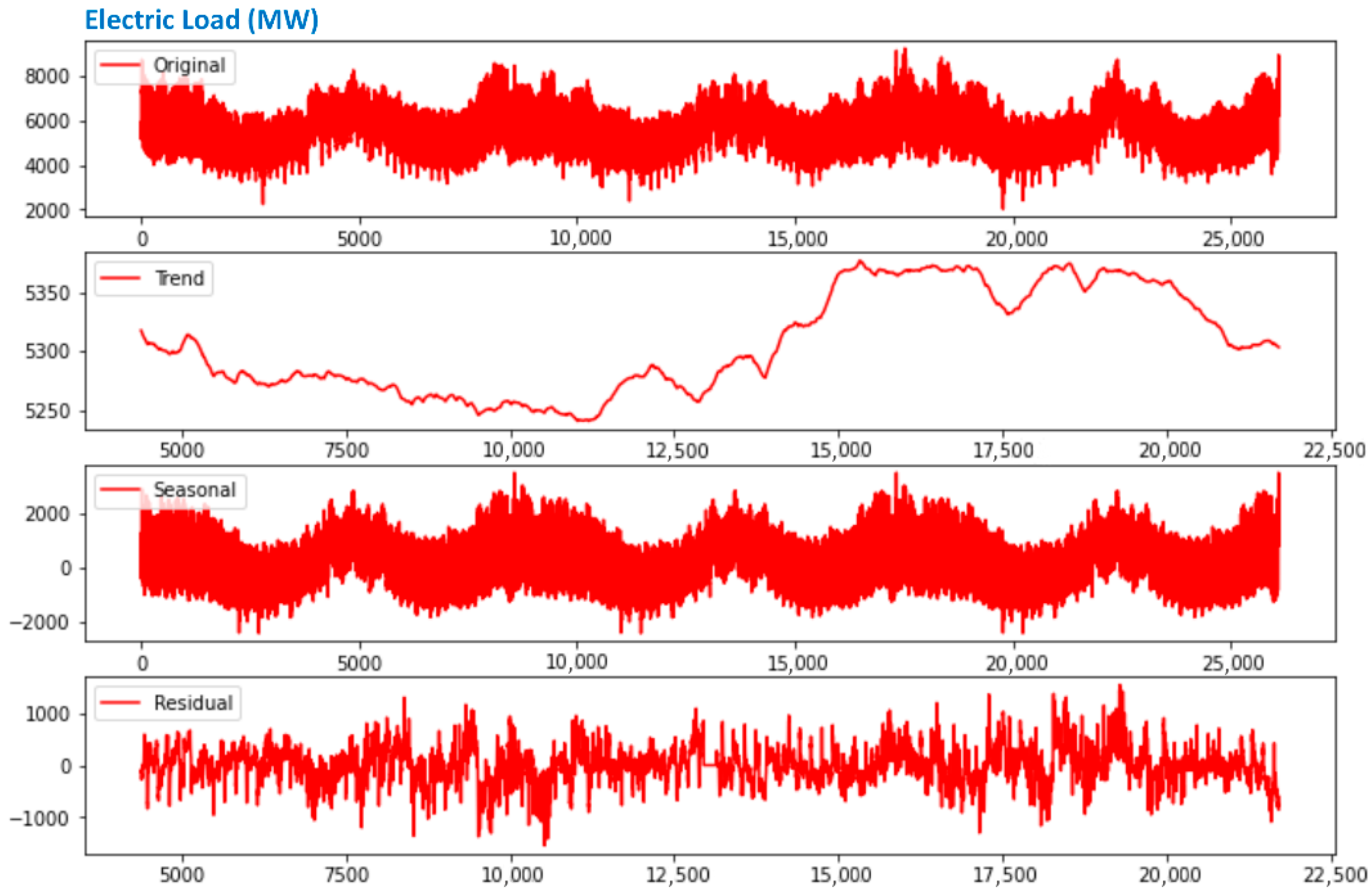
• Seasonality in time-series data represents recurring patterns that appear at consistent intervals—such as daily, weekly, monthly, or annually. This feature is common across various datasets, including those related to sales, weather, and transportation. Recognizing seasonal patterns is crucial for precise forecasting and uncovering hidden trends within the data.
• Trend refers to the overall direction in which time-series data move over an extended period—whether upward, downward, or stable. It reflects long-term behavior and may be influenced by factors such as economic shifts or demographic changes. Detecting trends is essential for understanding the data’s structure and generating reliable forecasts. Techniques like linear regression, moving averages, and exponential smoothing are commonly used to identify trends. Additionally, trends may shift over time—a phenomenon known as a change point—which analysts should be mindful of during analysis
• Cyclic behavior involves patterns in time-series data that repeat over periods longer than seasonal cycles, often spanning several years. These cycles may be driven by macro-level factors such as economic trends. For instance, indicators like GDP, employment, and production often display cyclic behavior in economic data. Recognizing these cycles aids in grasping deeper data patterns and improving prediction accuracy.
• Irregular fluctuations refer to random or unexpected variations in a time series that cannot be attributed to trend, seasonality, or cycles. Such irregularities may arise from unpredictable events like natural disasters or sudden shifts in demand. Understanding these anomalies is important for fully interpreting the data and enhancing the accuracy of forecasts.

To emphasize the features of the load time series, Figure 5 presents boxplots of the training dataset. The plots clearly reveal cyclical behavior, indicating the presence of seasonality.

A yearly recurring pattern is easy to identify because a full year contains 8760 h, and the pattern recurs roughly every 9000 data points. In winter, load values span a wider range compared to other seasons, resulting in larger boxplots for that period. Additionally, within a calendar year, two seasons—winter and summer—show noticeable peaks in load, while the other two seasons exhibit noticeable troughs. The boxplots also reveal some load values that behave as outliers, which usually correspond to holidays, as shown in Section 4. These findings confirm the necessity of temporal models, like LSTM and GRU, that account for recurring seasonal fluctuations.

Figure 6 illustrates the trend and seasonal components of the training dataset. A clear upward trend is noticeable during 2014 and 2015 (when the sample index exceeds 10,000), reinforcing the importance of modeling nonstationary behavior. Regarding seasonality, sharp peaks in summer and winter can be identified, linked to energy-intensive periods where the cooling needs in summer and the heating needs in winter, respectively, rise. Accordingly, troughs are detected in the spring and autumn seasons.

Figure 7 shows the load data from the testing dataset (year 2016). As can be seen, energy demand continues to rise, in line with prior years. The same seasonal patterns occur, with noticeable peaks in winter and summer and lower demand during spring and autumn. Therefore, it can be argued that the training period can capture the representative dynamics for 2016, justifying generalization.

The workflow of the whole process is illustrated in Figure 8. The key stages from raw data acquisition to post-modeling analysis are summarized. The pipeline includes data preprocessing steps such as cleaning and normalization, the transformation of time series using a sliding window approach, and training the three prediction models. The datasets and the models’ outputs are further processed and visualized using Microsoft Power BI, as will be discussed in the sequel.

4. Experimental Results

4.1. Data Preprocessing and Visualization Based on the Power BI Tool

The Power BI data visualization software (v. 2.118.286.0) product constitutes a useful tool for handling the electric load forecasting problem. Developed by Microsoft, Power BI is primarily designed for business intelligence and is included in the Microsoft Power Platform [36]. It comprises a suite of software services, applications, and connectors that collaborate to transform diverse data sources into unified, visually engaging, and interactive insights. Users can import data directly from databases, websites, or structured file formats such as spreadsheets [37].

This dashboard allows the following:

• To inspect prediction errors by model, time, and day type;
• To perform visual inspection of high-error cases and model bias during specific time ranges;
• To toggle between models and horizons interactively.

In the sequel, this tool is used extensively to facilitate assessing the forecasting capabilities of the deep learning models by efficiently visualizing characteristic load curves and the predictors’ outputs. In this perspective, the original testing dataset was enriched with the following metadata: (a) year, (b) month, (c) day, (d) hour, (e) season, (f) weekday, and (g) date.

Figure 9 shows the Power BI’s screen for the training dataset. On the top of the screen, the following filters are distinguished:

• A drop-down list containing the four seasons.
• A horizontal moving bar that adjusts the limits of the electric load.
• A horizontal moving bar that adjusts the calendar of the training dataset.
• A dropdown list with the names of the seven weekdays.

Moreover, a significant feature of the tool is the Comparison button, which leads to the screen shown in Figure 10. Finally, there is a box below the filter area, which includes the following statistical measures of the time series: max, min, median, average, and sum. These values can change according to the choice of filters. Therefore, by selecting “winter” from the seasons and “Thursday” from the days, the values of the statistical measures for this season and day will substitute the ones shown in Figure 9.

It becomes evident from Figure 10 that all 3 years exhibit a similar load series pattern across the months. In spring and autumn, the demand for power is low, while it is increased during summer and winter. This behavior is considered normal for Greece, since in summer the larger amount of electricity is required for cooling purposes, while during winter, there is dual behavior due to heating purposes.

It is also worth mentioning that, according to Figure 11, the average load on Sundays is less than 5000 MWh, which can be attributed to the fact that in Greece, Sunday is a rest day and neither the industrial sector nor the commercial one operates. Moreover, high load demand obviously occurs on weekdays and particularly on Thursdays, while Saturday is considered to be a transition day, since until early in the evening, its pattern is more similar to that of a weekday.

4.2. Results and Analysis

All models were developed using Python (v. 3.12) and Keras API (v. 2.18.0) on top of TensorFlow. Training was conducted in Google Collaboratory using GPU acceleration (K80, 12 GB RAM). The testbed includes the RNN, LSTM and GRU predictors, whose structural characteristics are shown in

Table 1. Structural and learning characteristics set for the predictors.

Number of layers	2
Neurons per layer	40, 100, 150, 200, 400, 500
Input length (hours)	6, 12, 32, 48, 48, 96, 168
Forecast horizon	1, 2, 24
Batch size	12–360
Optimizer	Adam
Drop-out	0.35
Error function	Root Mean Squared Error
Bias	Yes
Learning rate	0.001

. In order to address training variance due to the random weight initialization, each experiment was executed five times, and the results were averaged. The learning characteristics, common to all the competing predictors, are also included in Table 1. For each one of the predictors, experiments were conducted for the whole set of combinations of the structural features, as well as for all the combinations of input lengths and batch sizes.

4.2.1. One-Step-Ahead Prediction: Overall Performance and Comparative Analysis

As far as the main forecasting horizon of one-hour ahead is concerned, the performance measures for the three deep learning models are illustrated in

Table 2. Best 5 models from each architecture.

Model	Neurons	Parameters	Batch Size	Input Length	Time (s)	RMSE	MAPE
(1) GRU	200	363,201	16	32	487	83.2	1.18
(2) GRU	500	3,006,501	16	32	348	83.4	1.18
(3) LSTM	500	3,006,501	16	32	585	83.8	1.18
(4) GRU	200	363,201	16	32	273	83.6	1.19
(5) GRU	400	1,925,201	12	48	524	86.1	1.23
(6) LSTM	200	482,601	16	32	505	86.7	1.23
(7) LSTM	200	482,601	12	48	545	87.8	1.24
(8) LSTM	150	271,950	12	48	662	88.2	1.25
(9) LSTM	400	1,925,201	12	48	761	87.9	1.26
(10) GRU	150	271,951	12	48	525	88.7	1.27
(11) RNN	200	120,801	80	48	330	115.1	1.71
(12) RNN	40	4961	24	48	808	115.4	1.73
(13) RNN	40	4961	24	96	504	118.2	1.74
(14) RNN	200	120,801	120	96	1389	123.1	1.82
(15) RNN	40	4961	240	168	519	130.48	1.92

, where the best five performances of each model are shown, along with the training time. The results are sorted in ascending order in terms of MAPE. It should be noted that in all three network categories the two-layer structures provided the best results and are included in the list below.

According to the above results, GRUs exhibit superior performance compared to LSTMs and RNNs in runtime efficiency and forecasting accuracy at one-hour-ahead forecasting. Its simplified gating mechanism allowed it to maintain temporal dependencies efficiently. While LSTM offered similar accuracy, its higher training time and memory consumption make it less suitable for real-time forecasting unless resources are abundant. RNNs show moderate accuracy, even with longer input vectors. Accordingly, the behavior of the best GRU forecaster is further investigated.

The best GRU predictor attained an RMSE of 83.2 MW and a MAPE of 1.18%. Moreover, the absolute error on the test dataset yields a yearly average error of 59.1 MW, with a standard deviation of 57.6 MW. This means that for the majority of the 8784 h in 2016, the prediction error remained below 117 MW, indicating that the forecasting model delivers consistently reliable performance.

In order to validate the predictors’ performances, the 95% confidence intervals for the fifteen models presented in Table 2 are given in

Table 3. The 95% confidence intervals for the best 5 models from each architecture.

Model	RMSE (Lower Bound)	RMSE (Upper Bound)	MAPE (Lower Bound)	MAPE (Upper Bound)
(1) GRU	81.9	84.4	0.74	1.41
(2) GRU	82.1	84.6	0.75	1.44
(3) LSTM	82.3	85.3	0.72	1.48
(4) GRU	80.1	87.1	0.75	1.53
(5) GRU	84.6	87.5	0.75	1.47
(6) LSTM	83.8	89.6	0.76	1.59
(7) LSTM	84.6	90.8	0.76	1.57
(8) LSTM	84.8	91.6	0.72	1.59
(9) LSTM	83.9	91.8	0.74	1.61
(10) GRU	83.6	93.8	0.78	1.55
(11) RNN	94.9	135.2	1.41	2.02
(12) RNN	111.8	118.9	1.67	1.79
(13) RNN	111.6	124.7	1.64	1.84
(14) RNN	103.8	142.3	1.52	2.12
(15) RNN	105.0	155.9	1.55	2.29

. According to the results, the best models given in Table 2 attained the narrowest confidence intervals in terms of RMSE. Additionally, in terms of MAPE, the worst upper bound for the GRU and the LSTM models was 1.61%, significantly lower than 2%, which is considered to be the limit for an accurate electric load prediction. As far as RNNs are concerned, the five representatives exhibit confidence intervals with a greater variety of widths than their competing rivals. It should be noticed that case (12) outperforms its rivals on both metrics.

The prediction performance of the GRU model is reinforced by the absolute error duration curve shown in

Table 4. Absolute error duration curve for the GRU forecaster.

Error in MW	>100	>200	>400	>500
Hours	1481	239	58	9
Time percentage	16.86%	2.72%	0.66%	0.10%

. This curve illustrates the percentage of hours in 2016 during which the absolute forecasting error exceeded the threshold values listed in the first row. The results indicate that the GRU forecaster performs very well, with forecast errors staying below 100 MW and 200 MW for over 83% and 93% of the time, respectively. Moreover, large errors exceeding 500 MW occurred only nine times during the entire year.

A typical week is depicted in Figure 12. It contains data from 12 June to 18 June 2016. As can be seen, for the load curve of the Greek power system, the magnitude of the extremal loads as well as the relative position of the peak loads are important factors for describing the load curve profile of a particular day type. The actual load curves are in blue, and the GRU’s predicted values are plotted in red. The different weekdays and Sunday are clearly distinguished.

4.2.2. One-Step-Ahead Prediction: Seasonal and Day-Type Performance—Special Days

In the sequel, the GRU forecaster’s performance in terms of seasonal forecasts is assessed and the metrics for the four seasons are shown in

Table 5. Seasonal performance for the GRU forecaster.

Season	MAPE Testing	RMSE Testing
Winter	1.21%	92.4
Spring	1.31%	82.1
Summer	0.89%	55.3
Autumn	1.25%	89.9

. Although a single model is used to predict the entire year, the model maintains an error rate well below 2% across all seasons. Summer emerges as the most accurately predicted season, while the remaining three seasons show comparable RMSE and MAPE values.

In order to focus on particular day types across all seasons, the load curves for weekdays and Sundays are illustrated in Figure 13, Figure 14, Figure 15, Figure 16, Figure 17, Figure 18, Figure 19 and Figure 20.

According to the graphs above, the following comments are in order:

• On working days, the morning and evening peak loads, as well as the first minimum load, show a consistent pattern across all seasons. However, during spring and autumn working days, the evening minimum is more clearly defined compared to winter and summer.
• As far as Sundays are concerned, the load curve differs significantly from that of working days, both in shape and seasonal variation. Notably, after 6 p.m., the Sunday load curves in autumn and spring resemble those of their corresponding working days.
• Although there are some variations in both seasonal trends and day types, the deep learning prediction model effectively captures the actual load curves, accurately identifying the peak and minimum values. Sundays pose a greater challenge for prediction due to lower demand and differing social behavior. Nevertheless, GRU performs well in monitoring the shift between weekends and working days.

Orthodox Easter and Assumption Day (15 August) are two days in the Greek calendar with high irregularity. The corresponding load curves are shown in Figure 21 and Figure 22. On both days, the morning peak is absent and electricity demand continues to decline until 3 p.m. Notably, on Easter, the load drops to a significantly low level (2331 MW at 3 p.m.) compared to the same time on the previous day (3405 MW) or the previous Sunday (3392 MW), resulting in substantial forecasting errors. This unusual pattern is largely due to the specific nature of these days in Greece, where industrial and household activities are minimal. Moreover, Easter usually falls in the middle of Spring, where the weather is mild and the need for heating or cooling is reduced.

A comparable trend is observed on Assumption Day, during which the GRU forecaster struggles to provide accurate predictions until around 4 p.m. While it captures the overall dynamics, large errors persist. This is primarily because many Greeks are on vacation and spend most of the morning and midday hours outdoors. However, once the load curve normalizes around 4 p.m., the forecaster’s accuracy improves significantly. In summary, the GRU’s performance, which is similar to those of LSTM and RNN for these particular days, is decreased, and the forecaster is unable to capture such irregular demand patterns without additional context about the specifics of these days.

4.2.3. One-Step-Ahead Prediction: A Generalization Scenario

In an attempt to investigate the generalization capabilities of the GRU forecaster, an alternative scenario is presented in the sequel. A time period from the COVID-19 era is examined; particularly, a two-week period spanning from a week before the second lockdown in Greece (which started on 7 November 2020) to a week after the initiation of the lockdown. The GRU, which has already been trained using data from 2013 to 2015, is applied to this small dataset, and the predicted load curve (red line) is shown in Figure 23, along with the actual electric load (blue line). Predictions from the seventh and the eighth of November are also given in Figure 24 and Figure 25, respectively.

According to the graphs, on 7 November, the predictor slightly overestimates for the first part of the day but manages to capture the actual load curve after that. On November 8th and for the rest of the week afterwards, the predictor’s accurately identifies the time series. For this two-week period, GRU attains an RMSE of 103.13 MW and a MAPE score of 1.60%, below the 2% threshold. From the results, it is concluded that even though the testing data were more than four years apart from the training data, the trained GRU predictor performed adequately.

4.2.4. Two- and Twenty-Four-Step-Ahead Prediction

In the sequel, the three competing rivals are examined in performing 2 h and 24 h ahead predictions.

Table 6. Best 5 models from RNN, LSTM, and GRU architectures for 2-step (hours)-ahead prediction.

Model	Neurons	Parameters	Batch Size	Input Length	RMSE	MAPE
GRU	200	363,201	12	96	121.7	1.69
LSTM	200	482,601	12	96	131.4	1.83
GRU	200	363,201	12	24	132.8	1.85
LSTM	200	482,601	12	168	133.6	1.87
GRU	200	363,201	12	48	134.5	1.88

and

Table 7. Best 5 models from the RNN, LSTM and GRU architectures for 24-step-ahead prediction.

Model	Neurons	Parameters	Batch Size	Input Length	RMSE	MAPE
GRU	200	363,201	24	168	343.9	4.67
RNN	200	330,824	96	168	362.2	5.12
GRU	40	41,544	24	168	380.1	5.32
GRU	200	363,201	96	168	380.3	5.40
RNN	40	14,984	48	168	374.9	5.44

show the best five performances for the 2 h ahead and the 24 h ahead cases, respectively. The results are also sorted in ascending order in terms of MAPE. Moreover, in

Table 8. MAPE for 24-step-ahead prediction for various input vectors.

Model	Neurons	24 Inputs	48 Inputs	96 Inputs	168 Inputs
RNN	40	6.04	6.09	5.78	5.44
LSTM	40	6.74	6.78	6.61	6.16
GRU	40	6.13	6.06	5.84	5.32
Model	Neurons	24 Inputs	48 Inputs	96 Inputs	168 Inputs
RNN	200	5.86	5.77	6.11	5.12
LSTM	200	6.40	6.42	6.26	5.49
GRU	200	5.72	5.60	5.69	4.75

, results for certain architectures and input vectors for the case of 24-step-ahead prediction are illustrated.

As can be seen from Table 6, the RNN model is not included in the best performances, in accordance with the findings of 1 h ahead predictions. Additionally, the rest of the competing rivals perform similarly, with the GRU models being less complex.

An interesting observation stems from the fact that the input lengths are much bigger than those reported in the one-step-ahead case (32 to 48 for the best five performances). Therefore, it can be argued that, even though the forecasting horizon was enlarged by merely one hour, the need for more temporal information has been increased. However, using longer input vectors improves results up to a saturation point. Even from the third best performance, the input length varies and cannot be considered a significant factor.

Proceeding to the broader forecasting horizon of 24 steps ahead, the following conclusions are drawn from the results shown in Table 7:

• The GRU predictor that appears in the first, third, and fourth places in the tables exhibits the best performance, a finding that is consistent with the particular forecaster in the previous two cases.
• The LSTM does not appear in Table 7. In fact, the best LSTM performance is the seventh best among all predictors.
• The RNN appears two times in Table 7 and holds the sixth place as well, attaining similar prediction errors with those of GRU.
• The longest input vector contributed to the best performances. Therefore, in the 24 h forecast horizon, the deep learning models require prior knowledge from the same day of the previous week.
• The reported values prove that the broader forecasting horizon leads to predictions that are far from being accurate, since a MAPE greater than 2% does not correspond to trustworthy predictions. The information that can be extracted from this kind of prediction is limited to the trend of the next day’s load curve.

Table 8 illustrates the performance of the three forecasters for two specific configurations and for several input vectors. The conclusions drawn from these results are consistent with the aforementioned, since the RNN’s performance is comparable or superior to GRU for the 40-neuron configuration and for simpler input vectors for the 200-neuron configuration. Moreover, LSTM comes third in both cases. Finally, the performance of GRU and LSTM is ameliorated as the size of the input vector increases in both configurations. However, in the case of RNNs, a correlation between the performance and size of the input vector cannot be distinguished. In the case of 200 neurons per layer, all three models attained their best performance for the longest input vector.

The typical week shown in Figure 12 is presented in Figure 26 and Figure 27, for the cases of 2-step-ahead and 24-step-ahead prediction with the GRU model, respectively. In the case of 2-steps ahead, there exists a difference mainly in the extremal points and, obviously, on Sunday. As far as the 24-step-ahead case is concerned, the predictor identifies the dynamics of the time series to a certain degree, but it fails to accurately identify its values, particularly in regions with fluctuations.

From the aforementioned analysis, it becomes evident that the longer the forecasting horizon, the greater the need for exogenous inputs, like climate or environmental variables, since the past load values themselves cannot lead to effective and adequate forecasts.

5. Conclusions

This study presented a comparative evaluation of three deep learning architectures—RNN, LSTM, and GRU—for short-term load forecasting, using real data from the Greek power grid. The models were assessed over multiple forecasting horizons (1 h, 2 h, and 24 h), with a special emphasis on performance under irregular conditions such as public holidays and weekends.

The findings confirm the ability of recurrent deep learning models to handle temporal dependencies inherent in electric load data. Among them, the GRU model consistently outperformed its counterparts, delivering the lowest RMSE and MAPE values while maintaining faster training times. LSTM achieved comparable accuracy but required more computational resources, while traditional RNNs were hindered by vanishing gradient issues.

Other findings from this study include the following:

• Integration of forecasting models with an interactive Power BI dashboard for real-time visualization and decision support.
• Systematic exploration of model configurations, input/output vector lengths, and training parameters to fine-tune performance.

Despite the robust outcomes, the models showed some limitations in handling atypical scenarios such as holidays and abrupt demand changes. These findings emphasize the need for hybrid approaches combining deep learning with rule-based logic, thus incorporating explicit encoding or external features like weather or policy effects.

Future work should focus on the following:

• Incorporating multivariate inputs such as temperature, mobility, and electricity price.
• Exploring hybrid and attention-based models (e.g., transformers) to improve long-range prediction fidelity.
• Applying explainability tools (e.g., SHAP and LIME) to enhance trust and transparency in decision support.

In conclusion, this study demonstrates that GRU- and LSTM-based models provide effective and scalable solutions for operational STLF in modern power systems, especially when integrated into human-centric visualization platforms.

References

1. Hoang, A.; Vo, D. The balanced enegy mix for achieving environmental and economic goals in the long run. Energies 2020, 13, 3850. [Google Scholar] [CrossRef]
2. Marneris, I.; Ntomaris, A.; Biskas, P.; Basilis, C.; Chatzigiannis, D.; Demoulias, C.; Oureilidis, K.; Bakirtzis, A. Optimal Participation of RES aggregators in energy and ancillary services markets. IEEE Trans. Ind. Appl. 2022, 59, 232–243. [Google Scholar] [CrossRef]
3. Lychnaras, V.; Passas, C. The Greek enery sector and the impact of natural gas process on domestic electricity prices. Greek Econ. Outlook 2023, 51, 74–86. [Google Scholar]
4. Perçuku, A.; Minkovska, D.; Hinov, N. Enhancing electricity load forecasting with machine learning and deep learning. Technologies 2025, 13, 59. [Google Scholar] [CrossRef]
5. Dudek, G. Pattern-based local Linear Regression models for short-term load forecasting. Electr. Power Syst. Res. 2016, 130, 139–147. [Google Scholar] [CrossRef]
6. Park, D.C.; El-Sharkawi, M.; Marks, R.; Atlas, L.; Damborg, M. Electric load forecasting using an artificial neural network. IEEE Trans. Power Syst. 1991, 6, 442–449. [Google Scholar] [CrossRef]
7. Papalexopoulos, A.; How, S.; Peng, T. An implementation of a neural network based load forecasting model for the EMS. IEEE Trans. Power Syst. 1994, 9, 1956–1962. [Google Scholar] [CrossRef]
8. Bakirtzis, A.; Theocharis, J.; Kiartzis, S.; Satsios, K. Short-term load forecasting using fuzzy neural networks. IEEE Trans. Power Syst. 1995, 10, 1518–1524. [Google Scholar] [CrossRef]
9. Bansal, R. Bibliography on the fuzzy set theory applications in power systems. IEEE Trans. Power Syst. 2003, 18, 1291–1299. [Google Scholar] [CrossRef]
10. Mastorocostas, P.; Theocharis, J.; Bakirtzis, A. Fuzzy modeling for short-term load forecasting using the orthogonal least squares method. IEEE Trans. Power Syst. 1999, 14, 29–36. [Google Scholar] [CrossRef]
11. Shah, S.; Nagraja, H.; Chakravorty, J. ANN and ANFIS for short term load forecasting. Eng. Technol. Appl. Sci. Res. 2018, 8, 2818–2820. [Google Scholar] [CrossRef]
12. Kandilogiannakis, G.; Mastorocostas, P.; Voulodimos, A. ReNFuzz-LF: A recurrent neurofuzzy system for short-term load forecasting. Energies 2022, 15, 3637. [Google Scholar] [CrossRef]
13. Giasemidis, G.; Haben, S.; Lee, T.; Singleton, C.; Grindrod, P. A genetic algorithm approach for modelling low voltage network demands. Appl. Energy 2017, 203, 463–473. [Google Scholar] [CrossRef]
14. Yang, Y.; Shang, Z.; Chen, Y.; Chen, Y. Multi-objective particle swarm optimization algorithm for multi-step electric load forecasting. Energies 2020, 13, 532. [Google Scholar] [CrossRef]
15. Zhao, H.; Tang, R.; He, Z. Research on short-term power load forecasting based on APSO-SVR. In Proceedings of the 6th International Conference on Control and Robots, Intelligent Control and Artificial Intelligence (RICAI), Nanking, China, 6–8 December 2024. [Google Scholar] [CrossRef]
16. Bianchi, F.; Maiorino, E.; Kampffmeyer, M.; Rizzi, A.; Jenssen, R. Recurrent Neural Networks for Short-Term Load Forecasting—An Overview and Comparative Analysis; Springer: Cham, Switzerland, 2017. [Google Scholar] [CrossRef]
17. Hochreiter, S.; Schmidhuber, J. Long short-term memory. Neural Comput. 1997, 9, 1735–1780. [Google Scholar] [CrossRef] [PubMed]
18. Cho, K.; van Merriënboer, B.; Gulcehre, C.; Bahdanau, D.; Bougares, F.; Schwenk, H.; Bengio, Y. Learning phrase representations using RNN encoder–decoder for statistical machine translation. arXiv 2014, arXiv:1406.1078. [Google Scholar] [CrossRef]
19. Yu, K. Adaptive Bi-directional LSTM short-term load forecasting with improved attention mechanisms. Energies 2024, 17, 3709. [Google Scholar] [CrossRef]
20. Ullah, K.; Ahsan, M.; Hasanat, S.M.; Haris, M.; Yousaf, H.; Raza, S.F. Short-term load forecasting: A comprehensive review and simulation study with CNN-LSTM hybrid approach. IEEE Access 2024, 12, 111858–111881. [Google Scholar] [CrossRef]
21. Wang, Y.; Zhang, N.; Chen, X. A short-term residential load forecasting model based on LSTM RNN considering weather. Energies 2021, 14, 2737. [Google Scholar] [CrossRef]
22. Abumohse, M.; Owda, A.; Owda, M. Electrical load forecasting using LSTM, GRU, and RNN algorithms. Energies 2023, 16, 2283. [Google Scholar] [CrossRef]
23. Guo, X.; Gao, Y.; Song, W.; Zen, Y.; Shi, X. Short-term power load forecasting based on CEEMDAN-WT-VMD joint denoising and BiTCN-BiGRU-Attention. Electronics 2025, 14, 1871. [Google Scholar] [CrossRef]
24. Hasanat, S.; Ullah, K.; Yousaf, H.; Munir, K.; Abid, S.; Bokhari, S.A.S. Enhancing Short-term load forecasting with a CNN-GRU hybrid model: A comparative analysis. IEEE Access 2024, 12, 184132–184141. [Google Scholar] [CrossRef]
25. Pirbazari, A.; Chakravorty, A.; Rong, C. Evaluating feature selection methods for short-term load forecasting. In Proceedings of the 2019 IEEE International Conference on Big Data and Smart Computing, Kyoto, Japan, 27 February–2 March 2019. [Google Scholar] [CrossRef]
26. Yang, Y.; Wang, Z.; Gao, Y.; Wu, J.; Zhao, S.; Ding, Z. An effective dimensionality reduction approach for short-term load forecasting. Electr. Power Syst. Res. 2022, 210, 108150. [Google Scholar] [CrossRef]
27. Rodriguez, F.; Cardeire, C.; Calado, J.; Melicio, R. Short-term load forecasting of electricity demand for the residential sector based on modelling techniques: A systematic review. Energies 2023, 16, 4098. [Google Scholar] [CrossRef]
28. Hasan, M.; Mifta, Z.; Papiya, S.J.; Roy, P.; Dey, P.; Salsabil, N.A.; Chowdhury, N.-U.-R.; Farrok, O. A state-of-the-art comparative review of load forecasting methods: Characteristics, perspectives, and applications. Energy Convers. Manag. X 2025, 26, 100922. [Google Scholar] [CrossRef]
29. Géron, A. Hands-On Machine Learning with Scikit-Learn, Keras, and TensorFlow; O’Reilly Media: Sebastopol, CA, USA, 2019. [Google Scholar]
30. Mienye, I.; Swart, T.; Obaido, G. Recurrent neural networks: A comprehensive review of architectures, variants, and applications. Information 2024, 15, 517. [Google Scholar] [CrossRef]
31. Bouktif, S.; Fiaz, A.; Ouni, A.; Serhani, M. Optimal deep learning LSTM model for electric load forecasting using feature selection and genetic algorithm: Comparison with machine learning. Energies 2018, 11, 1636. [Google Scholar] [CrossRef]
32. Agrawal, V.; Goswami, P.; Sarma, K. Week-ahead forecasting of household energy consumption using CNN and multivariate data. WSEAS Trans. Comput. 2021, 20, 182–188. [Google Scholar] [CrossRef]
33. Greek Independent Power Transmission Operator. Available online: https://www.admie.gr/en/market/market-statistics/detail-data (accessed on 10 May 2025).
34. Fatima, S.; Rahimi, A. A review of time-series forecasting algorithms for industrial manufacturing systems. Machines 2024, 12, 380. [Google Scholar] [CrossRef]
35. Seabold, S.; Perktold, J. Statsmodels: Econometric and statistical modeling in Python. In Proceedings of the 9th Python in Science Conference, Austin, TX, USA, 28 June–3 July 2010. [Google Scholar] [CrossRef]
36. Powell, B. Mastering Microsoft Power BI: Expert Techniques for Effective Data Analytics and Business Intelligence; Packt Publishing: Birmingham, UK, 2018. [Google Scholar]
37. Silva, R.F. Power BI—Business Intelligence Clinic: Create and Learn; Independently Published, 2018. [Google Scholar]
Figure 1. A typical RNN architecture.
Electronics 14 02820 g001
Figure 2. Configuration of an LSTM cell.
Electronics 14 02820 g002
Figure 3. Configuration of a GRU cell.
Electronics 14 02820 g003
Figure 4. The sliding window setup for the dropped, training, and forecasting data.
Electronics 14 02820 g004
Figure 5. Boxplots for the training dataset (2013–2015 period).
Electronics 14 02820 g005
Figure 6. Trend and seasonal components of the training dataset (2013–2015 period).
Electronics 14 02820 g006
Figure 7. Trend and seasonal components of the testing dataset (2016 period).
Electronics 14 02820 g007
Figure 8. Workflow diagram.
Electronics 14 02820 g008
Figure 9. The training dataset (2013–2015 period) in Power BI.
Electronics 14 02820 g009
Figure 10. The testing dataset (2016 period) in Power BI.
Electronics 14 02820 g010
Figure 11. Load demand on Sundays in Power BI.
Electronics 14 02820 g011
Figure 12. The load curve of a summer week. The actual load curves are in blue, and the GRU’s predicted values are plotted in red.
Electronics 14 02820 g012
Figure 13. Winter weekday. The actual load curves are in blue, and the GRU’s predicted values are plotted in red.
Electronics 14 02820 g013
Figure 14. Spring weekday. The actual load curves are in blue, and the GRU’s predicted values are plotted in red.
Electronics 14 02820 g014
Figure 15. Summer weekday. The actual load curves are in blue, and the GRU’s predicted values are plotted in red.
Electronics 14 02820 g015
Figure 16. Autumn weekday. The actual load curves are in blue, and the GRU’s predicted values are plotted in red.
Electronics 14 02820 g016
Figure 17. Winter Sunday. The actual load curves are in blue, and the GRU’s predicted values are plotted in red.
Electronics 14 02820 g017
Figure 18. Spring Sunday. The actual load curves are in blue, and the GRU’s predicted values are plotted in red.
Electronics 14 02820 g018
Figure 19. Summer Sunday. The actual load curves are in blue, and the GRU’s predicted values are plotted in red.
Electronics 14 02820 g019
Figure 20. Autumn Sunday. The actual load curves are in blue, and the GRU’s predicted values are plotted in red.
Electronics 14 02820 g020
Figure 21. Easter day. The actual load curves are in blue, and the GRU’s predicted values are plotted in red.
Electronics 14 02820 g021
Figure 22. Assumption Day. The actual load curves are in blue, and the GRU’s predicted values are plotted in red.
Electronics 14 02820 g022
Figure 23. The load curve of the COVID-19 period. The actual load curves are in blue, and the GRU’s predicted values are plotted in red.
Electronics 14 02820 g023
Figure 24. Load curve for 7 November 2020. The actual load curves are in blue, and the GRU’s predicted values are plotted in red.
Electronics 14 02820 g024
Figure 25. Load curve for 8 November 2020. The actual load curves are in blue, and the GRU’s predicted values are plotted in red.
Electronics 14 02820 g025
Figure 26. The load curve of a summer week for 2-step-ahead prediction. The actual load curves are in blue, and the GRU’s predicted values are plotted in red.
Electronics 14 02820 g026
Figure 27. The load curve of a summer week for 24-step-ahead prediction. The actual load curves are in blue, and the GRU’s predicted values are plotted in red.
Electronics 14 02820 g027