Vehicle Trajectory Data Augmentation Using Data Features and Road Map

Abstract

With the advancement of intelligent transportation systems, vehicle trajectory data have become a key component in areas like traffic flow prediction, route planning, and traffic management. However, high-quality, publicly available trajectory datasets are scarce due to concerns over privacy, copyright, and data collection costs. The lack of data creates challenges for training machine learning models and optimizing algorithms. To address this, we propose a new method for generating synthetic vehicle trajectory data, leveraging traffic flow characteristics and road maps. The approach begins by estimating hourly traffic volumes, then it uses the Poisson distribution modeling to assign departure times to synthetic trajectories. Origin and destination (OD) distributions are determined by analyzing historical data, allowing for the assignment of OD pairs to each synthetic trajectory. Path planning is then applied using a road map to generate a travel route. Finally, trajectory points, including positions and timestamps, are calculated based on road segment lengths and recommended speeds, with noise added to enhance realism. This method offers flexibility to incorporate additional information based on specific application needs, providing valuable opportunities for machine learning in intelligent transportation systems.

1. Introduction

In recent years, the rapid development of intelligent transportation systems (ITS) and the growing need for urban mobility analysis have led to an increased focus on vehicle trajectory data. Trajectory data are essential for a wide range of applications, such as traffic flow prediction [1], route planning [2], and real-time traffic management [3]. The accurate analysis of vehicle trajectories enables better decision-making [4], thereby optimizing transportation systems [5] and reducing congestion [6]. Given the dynamic nature of traffic, tracking and analyzing vehicle trajectories is crucial for understanding traffic patterns and improving urban mobility. Thus, research on trajectory data has become indispensable in the advancement of smart cities and the optimization of transportation infrastructure.

However, despite its significance, there is a notable shortage of high-quality, publicly available trajectory datasets. The primary reasons for this scarcity stem from various issues such as privacy concerns, legal constraints, and the high costs of data collection and maintenance [7]. Additionally, due to network instability, device issues, and the cost of transmitting and storing data, there is a lack of high-quality, dense trajectory datasets [8]. Many governments and private entities are reluctant to release large-scale trajectory data due to privacy laws and fears of misuse, especially when dealing with personal information that can be easily traced back to individual users. Furthermore, the complex and often costly process of collecting comprehensive vehicle trajectory data through GPS tracking or sensors on a wide scale limits the availability of large, accurate datasets. As a result, researchers often find themselves constrained by the limited availability of suitable data, which hinders progress in both theoretical research and practical applications.

The increasing reliance on machine learning in transportation research further underscores the need for high-quality trajectory datasets. Machine learning models, especially those used for traffic prediction [9], pattern recognition [10], and autonomous driving [11], require vast amounts of diverse and accurate data for effective training [12]. Without sufficient data, these models cannot achieve high accuracy, and their generalizability across different traffic scenarios is significantly reduced. The demand for data in machine learning is immense, as algorithms not only need large volumes of data but also data that are varied and contain representative traffic conditions. Given the limitations of existing datasets, there is a pressing need to develop methods to augment trajectory data and create synthetic datasets that can effectively support machine learning tasks. The success of artificial intelligence (AI) products is often attributed to the models’ deep understanding of accumulated data, which allows them to inherently uncover data patterns and learn the correlations between data and tasks [13]. The concept of data augmentation emerged early in the development of deep learning. Data augmentation has been widely utilized and has proven to be both effective and efficient [14]. For instance, in LeNet [15], random distortions were applied to create nine times the number of distorted images, demonstrating that enlarging the training set can effectively reduce test error. Since then, data augmentation has become widely recognized as the best practice for training Convolutional Neural Networks (CNNs) [16]. AlexNet [17] explicitly incorporates several data augmentation techniques to mitigate overfitting. The study of trajectory data augmentation has gained increasing attention in recent years, as it plays a crucial role in addressing the challenges associated with data scarcity in transportation research.

Augmenting trajectory data involves generating new, realistic data points that can support the training of machine learning models, thereby enhancing their accuracy and generalizability. Yaksh J. Haranwala et al. proposed an innovative approach for augmenting trajectory data by applying geographical perturbations to the raw trajectory points along the path [18] and designed an open-source Python3 framework AugmenTRAJ for trajectory data augmentation [19]. He D. et al. proposed a method that concatenates existing trajectories to reconstruct a sufficient number of trajectories, effectively representing those that directly traverse the OD pair [20]. Jie Feng et al. extracted two features from the real data—sampling interval and spatial noise—to represent the generation process of raw trajectories [21]. Additionally, they are able to generate an arbitrary number of virtual trajectories based on the ground truth trajectories as needed. Xingrui Wang et al. proposed a map-based Two-Stage GAN method (TSG) to generate fine-grained and plausible large-scale trajectories [22].

Most of the existing trajectory data augmentation techniques are based on historical points, with a particular focus on applying position shifts or transformations. As we all know, these methods often leverage GPS data collected from past trajectories, where slight changes in position are made to create new samples. One common approach is to add noise to the trajectory points, or to use interpolation techniques to generate intermediate points between known trajectory segments. While these methods can increase the dataset’s size, they primarily rely on the assumption that the historical trajectory is a sufficient representation of future patterns, without accounting for the underlying structure of the road map or the broader context of traffic flow dynamics. Furthermore, trajectory data generation does not take into account the complex road network routing problem [23,24]. For example, techniques such as the use of Gaussian noise or random perturbations to simulate possible vehicle movements along a path are commonly applied. These methods are relatively simple and computationally efficient, but they may not accurately represent the full range of potential variations in trajectory data. They fail to incorporate the specific characteristics of the road map, such as road types, which can significantly influence the movement patterns of vehicles. As a result, the augmented trajectories generated by these methods might not capture the diversity of vehicle behaviors, limiting the applicability of the resulting data for advanced machine learning applications.

As transportation systems are inherently influenced by the structure and features of the road map, there is a growing need for trajectory augmentation methods that go beyond simple position shifts and instead incorporate road map and trajectory-specific characteristics into the augmentation data. In particular, trajectory augmentation methods that consider the relationship between the trajectory data and the underlying road map could provide more accurate and contextually relevant data. These approaches would ensure that the augmented trajectories not only vary in their positional coordinates but also adhere to the constraints imposed by the road map, such as permissible routes, road closures, or dynamic traffic patterns. Additionally, such techniques could take into account the characteristics of individual trajectories, such as their departure times, destinations, and travel speeds, offering a more personalized and data-driven augmentation approach.

To address these challenges, this study introduces a novel data augmentation technique for trajectory datasets. By leveraging the spatiotemporal distribution characteristics of traffic flow, along with road map and segment features, we generate simulated trajectory data. This approach extracts spatiotemporal distribution characteristics of traffic flow using historical data and uses road map features, aiming to produce high-quality synthetic data that enhances machine learning model performance and provides a more robust foundation for traffic analysis and ITS applications.

The main contributions of this work can be summarized as follows:

Proposed Framework for Simulated Trajectory Generation: A framework is introduced for generating simulated trajectory data based on macroscopic traffic flow characteristics. This approach extracts spatiotemporal distribution features from historical trajectory data, employs a Poisson distribution to simulate the time column, and generates subsequent trajectory points using path planning and edge information derived from the road map.

Systematic Process for Spatiotemporal Feature Extraction: A systematic process is provided for extracting spatiotemporal distribution features from real trajectory data. This includes steps for trajectory denoising, segmentation, and OD identification.

Integration with Road Network for Enhanced Classification: The method is grounded in the road network, enabling the attachment of precise classification information to the generated trajectory data. This supports the effective application of machine learning models in ITS.

Noise Injection in Spatial and Temporal Dimensions: A novel technique for adding noise to both spatial and temporal dimensions of the trajectory data is introduced, offering a fresh perspective on trajectory data simulation.

The remainder of this paper is structured as follows: Section 2 outlines the definitions related to the research problem and the methodologies used for trajectory data augmentation based on traffic flow characteristics and road maps. Section 3 presents the application of our system to a large mobility dataset. In Section 4, we discuss the advantages and limitations of the method. Finally, Section 5 provides the conclusion.

2. Materials and Methods

Firstly, we provide several definitions related to the research problem.

2.1. Definitions

Road map: The directed graph structure formed by the interconnection of various roads in the real world is the road map. The directed graph structure is composed of points and lines. The points in the road map represent the starting and ending points, or intersections, of the roads in the real world. The lines represent the road segments. We study the generation method of vehicle trajectory data. The road map refers to the road network composed of driving roads. Road map data is obtained through the open-source map project OpenStreetMap (OSM) [25].

Node: A node in a road map represents a starting or ending point, or an intersection, of a road in the real world. It is a two-dimensional point defined by longitude and latitude, which together indicates its location. Each node is assigned a unique OSM ID. The node’s geometry property stores its geographic information, specifically the point (longitude, latitude).

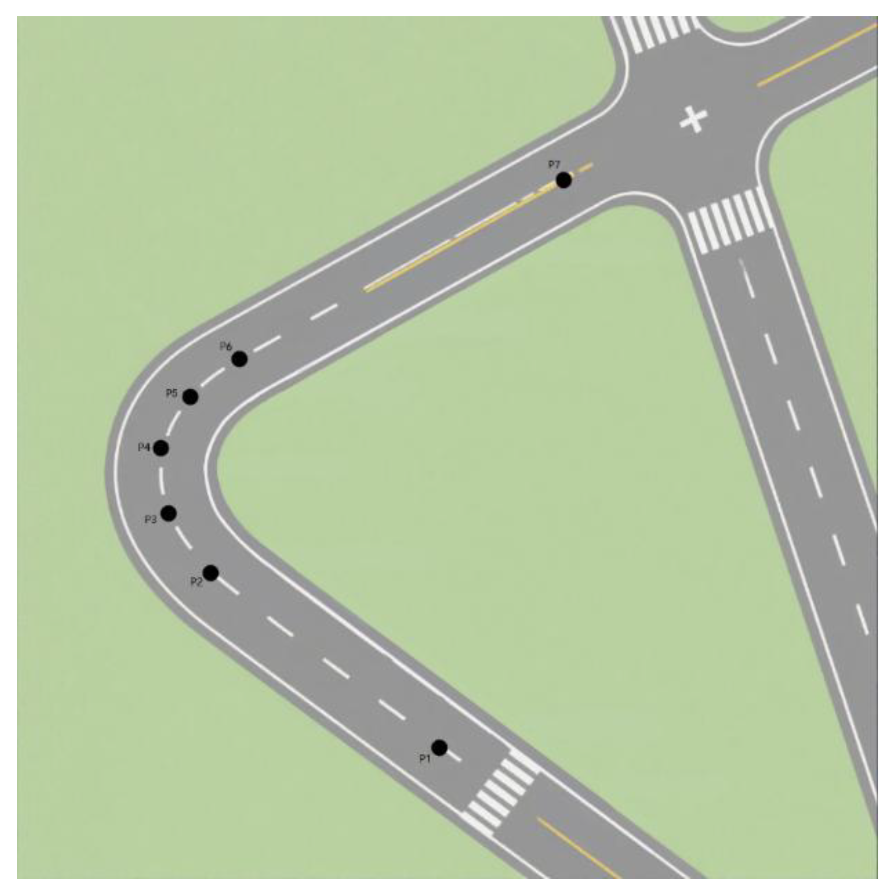
Edge: An edge in a road map represents a section of a road in the real world, connecting two adjacent nodes. Each edge stores the OSM IDs of its starting and ending nodes, as well as its own unique OSM ID. The geometry attribute of the edge contains its geographic information, represented as a series of connected points forming a LineString (longitude₁, latitude₁, longitude₂, latitude₂, …). Each point, denoted as p_i, defines a key point on the edge, with the edge being represented as edge = (p₁, p₂, p₃, …, p_n). These key points are determined by changes in the angle and curvature of the road. The segment between two adjacent key points is approximated as a straight line, as illustrated in Figure 1.

Edge length: This represents the distance a vehicle travels along the edge. It is calculated using the following method:

$$len\left(edge\right)=\sum _{i=1}^{n-1}len\left(p_i,p_{\left(i+1\right)}\right).$$

(1)

The term len(p_i, p_i+1) represents the circle distance between two adjacent points, calculated using the following method:

$$len\left(p_i, p_{i+1}\right)=2\mathrm{r}{\sin }^{-1}\sqrt{{\mathit{sin}}^2\left({\displaystyle \frac{\Delta \varphi }{2}}\right)+\mathit{cos}{\varphi }_1\mathit{cos}{\varphi }_2{\mathit{sin}}^2\left({\displaystyle \frac{\Delta \lambda }{2}}\right)},$$

(2)

r is the Earth’s radius (default 6,371,000 m);

ϕ₁, ϕ₂ are the latitudes of the two points (in radians);

$\Delta \varphi$, $\Delta \lambda$ are the differences in latitude and longitude (in radians).

Edge speed: The recommended driving speed on edge, influenced by factors such as road design and traffic flow. It is an inherent attribute of the edge, measured in kilometers per hour (km/h).

Route: A route represents the sequence of locations a vehicle passes through during a single trip, arranged in chronological order, with a unique move ID. It is represented by the ordered collection of nodes on the road map that the vehicle traverses, denoted as (n₁, n₂, n₃, …), where each n_i is the OSM ID of a road map node.

Trajectory Point: A trajectory point represents the position recorded by a vehicle along its path at specific time intervals. In the real world, these points are typically obtained using a GPS device. Each trajectory point includes at least three attributes: time, longitude, and latitude. In addition to these, our simulated trajectory points include two additional attributes: the path ID (moveid) and the road segment where the trajectory point is located, represented by the OSM IDs of the starting and ending nodes of the road segment (u, v).

2.2. Problem Statement

Given a set of GPS trajectories, we want to generate an arbitrary number of simulated trajectory data in the real-world area where these trajectories are distributed.

2.3. Methods

We generate simulated trajectory data based on the characteristics of historical trajectory data and the road map. Drawing on traffic engineering principles, we recognize that traffic volume exhibits spatiotemporal distribution patterns, that is, traffic volume is a random variable, and it fluctuates across different times and locations. These fluctuations follow certain regularities across various dimensions. The temporal distribution of trajectory data is primarily reflected in the predictable daily and hourly variations in traffic volume for specific cities or road segments. In this paper, by statistically analyzing the time distribution patterns of trajectory data, we determine the proportion of traffic volume for each day and hour within the simulation period. Using this information, we estimate the hourly traffic volume and then apply a Poisson distribution to allocate the trajectories across different time points within each hour, thereby determining the departure times for each simulated trajectory.

The spatial variation in traffic volume is characterized by its spatial distribution, reflecting how traffic volume differs across various sections of the road map. This variation is influenced by factors such as road grade, function, and location. To model this spatial distribution in simulated trajectories, we use methods such as OD surveys and path planning. Specifically, by statistically analyzing the OD data from historical trajectories, we determine the probability distribution of OD pairs and allocate starting and ending points for each simulated trajectory based on these distribution weights. Then, we employ multi-directional path planning functions (e.g., shortest time, shortest distance) on the road map to determine the driving route for each trajectory.

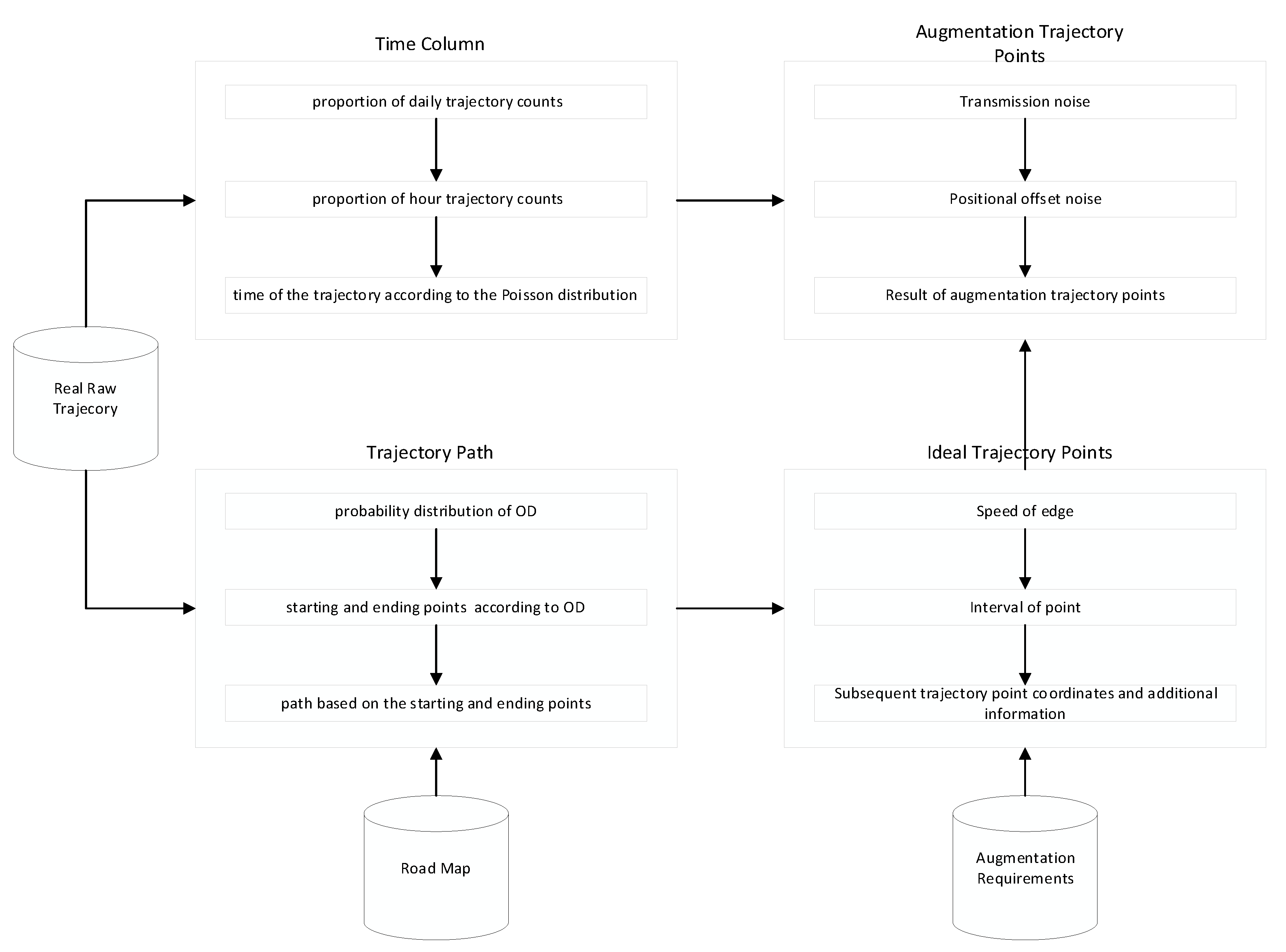
Once the driving route for the trajectory is determined, all the edges that the vehicle travels through during a single trip are identified. The edge length, recommended vehicle speed, and other attributes are then used to determine the positions of subsequent trajectory points and the corresponding timestamps under ideal conditions within specific intervals. Next, noise is applied to these ideal trajectory points to simulate real-world variations and generate the final trajectory data. The noise introduced includes transmission noise and positioning system noise that, respectively, affect the time and position attributes of the trajectory data. The overall process for generating trajectory data is illustrated in Figure 2.

2.3.1. Time Distribution Process of Simulated Trajectory Data

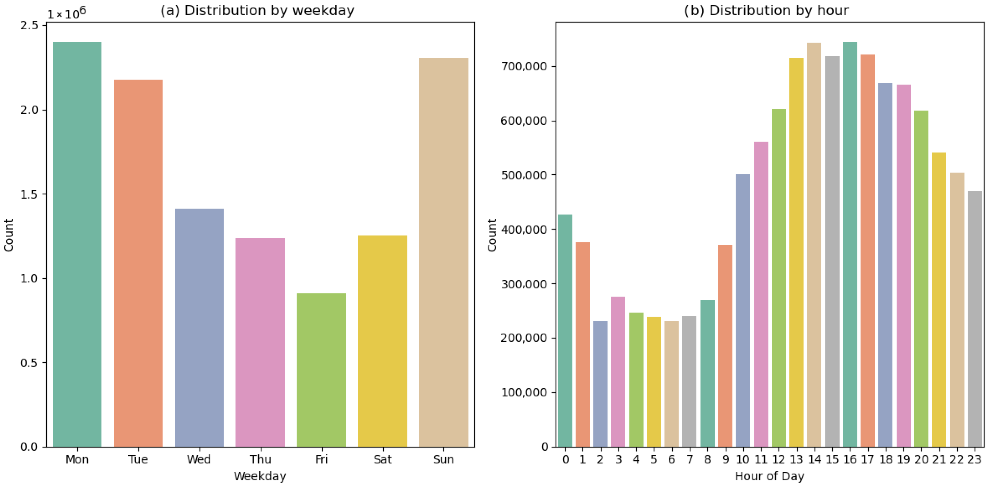
Traffic flow exhibits time variability, which is reflected in the changes in traffic patterns across different time periods. Each day of the week shows a certain degree of similarity in traffic flow distribution, such as the varying trends in flow between weekdays and weekends. Additionally, traffic flow distribution follows a certain pattern within each hour of the day, with heavier traffic during the morning and evening peak periods, while other times of the day remain relatively steady. However, on a shorter time scale, such as an hour or even a few minutes, the number of vehicle arrivals at a specific location exhibits randomness. Therefore, when simulating trajectory data, the distribution of data over time is determined based on historical data statistics of the trajectory flow in a macro context. On a micro level, we employ a Poisson distribution to model the specific arrival times of vehicles, reflecting the inherent randomness and uncertainty of traffic flow. Specifically, we simulate the time distribution of trajectory data through the following steps:

1. Set the total sum of the required generation trajectories and the time period t for the distribution of trajectory data (for example: from 14 April 2025 00:00:00 to 20 April 2025 23:59:59).

2. Traffic volume is a random variable with spatiotemporal distribution characteristics. The statistical granularity of traffic volume—such as by year, month, day, hour, and minute—is defined based on the needs of the trajectory data simulation. It is essential to determine the distribution and variation patterns within the simulated time period. Additionally, different vehicle types exhibit distinct travel patterns. For instance, the daily travel of operational vehicles generally follows a uniform distribution, while private car traffic is significantly lower during holidays compared to weekdays. Using statistical analysis of historical trajectories and predefined proportions, we derive the time distribution pattern of trajectory data. The granularity is set to the day of the week and hour, and the total number of trajectories is proportionally allocated across specific time periods.

The distribution of simulated trajectories across the days of the week is expressed as follows:

$$\sum _{i=0}^6{p}_i=1,$$

(3)

where p_i represents the proportional coefficient for the i-th day of the week.

The number of trajectories per day s_i (where i = 0, 1, 2, 3, 4, 5, 6) is expressed as follows:

$$s_i=sum\times p_i.$$

(4)

Similarly, during the 24 h of a day, the traffic volume in each hour is constantly changing. The time-varying law of traffic can be represented by the ratio of the traffic volume in a certain hour to the total traffic volume of the entire day.

And then, the number of trajectories in each hour is calculated based on the s_i determined in the previous step:

$$h_d=s_i\times q_d,$$

(5)

where $h_d$ (d = 0, 1, 2, 3, …, 23) represents the number of trajectories in the d-th hour and q_d represents the proportion coefficient of the traffic volume in the d-th hour to the total traffic volume of the entire day.

After the number of trajectories within each hour is determined, the departure time needs to be specified for each trajectory data. This corresponds to the start value of the time column in each augmented trajectory. The trajectory data simulated in this paper does not consider the traffic flow density, the mutual influence among vehicles, and other external interference factors. Thus, the arrival of vehicles is random to some extent. The vehicles arriving within a certain time interval are described by the Poisson distribution, which is in line with its statistical distribution characteristics. Mathematically, the distribution is represented as follows:

$$P(k)={\displaystyle \frac{{\left(\lambda t\right)}^k{e}^{-\lambda t}}{k!}}, k=0,1,2,\dots ,$$

(6)

where P(k) represents the probability of k vehicles reaching within time t, and λ represents the average number of vehicles reached per unit time interval (vehicles/s). The value of λ represents the number of arrivals per unit of time, which is calculated from the real trajectory data based on time statistics as previously described. t is the duration of each counting interval, and e is the base of the natural logarithm. However, when the total number of trajectories is large, the deviation can be ignored. The value of the “time” column in each row of the generated trajectory data can be set with the minimum timing granularity as required. We accurate it to the second, which is the time counting granularity adopted by most trajectory data.

As shown in

Table 1. Augmentation of time column.

Time	Lat	Lon	Moveid
14 April 2025 00:00:00	NaN	NaN	0
14 April 2025 00:00:05	NaN	NaN	1
14 April 2025 00:00:14	NaN	NaN	2
14 April 2025 00:00:17	NaN	NaN	3
14 April 2025 00:00:18	NaN	NaN	4
…	…	…	…
14 April 2025 00:59:57	NaN	NaN	1318

, the time distribution results simulate from the “00:00 on 14 April 2025, to 23:59:59 on 20 April 2025” time period based on historical data. A total of 100,000 trajectories were generated. Within one hour, trajectories were generated according to the Poisson distribution. The above process mainly determined the number of trajectories and their starting times within each time period. Among them, the moveid column was specified in the chronological order of the trajectories, and one moveid represents a travel record of a certain vehicle.

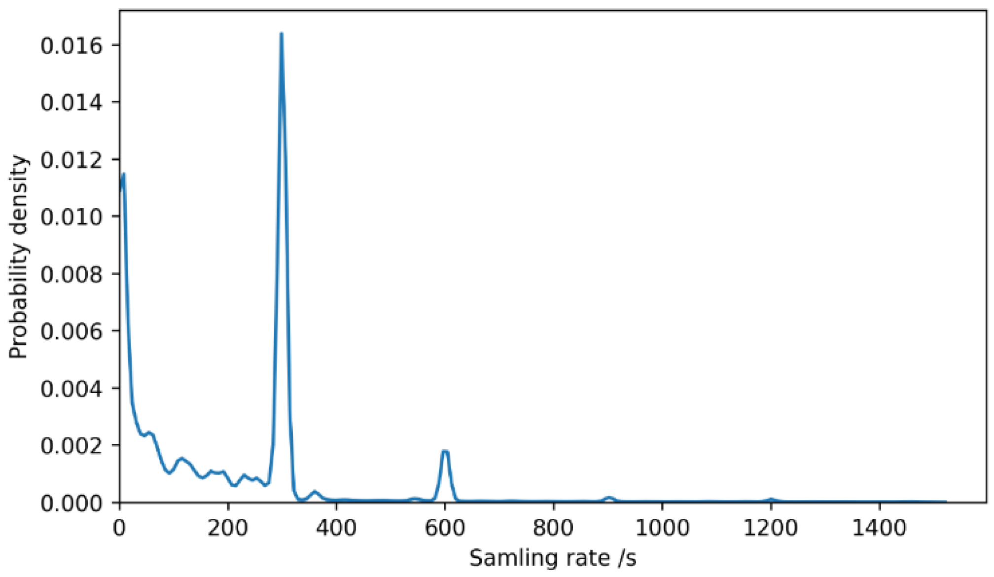
The sampling intervals of trajectory points in real trajectory data are different. The inherent attributes of different type sampling devices determine their own sampling intervals. When simulating trajectory data, the sampling interval of trajectory data determines the value of the time column of the remaining trajectory points after the starting point of a trajectory. When simulating trajectory data, to achieve a simulation effect, the sampling intervals of the trajectory data points in the real trajectory data can be statistically analyzed or they can be set according to the application scenarios of the simulated data, because different sampling intervals will affect the applicable scenarios of the data. For instance, if the sampling interval is 15 s, trajectory data can be used to analyze the starting and ending point information of the trip, the running speed of the vehicle, the delay at intersections, etc. If the sampling granularity is rough at, for example, one point every 15 to 30 min, then the trajectory data can only be used to analyze the general hotspot distribution of the vehicle.

2.3.2. Position Distribution Process of Simulated Trajectory Data

The generation of all trajectory points for a route is primarily divided into three steps. First, based on the OD statistical information from historical trajectory data, OD pairs are assigned to the trajectory points according to a probability distribution. Next, the path planning function of the road map is used to generate a driving route for each OD pair, which helps determine the set of all edges the vehicle travels through. Finally, based on the suggested speed of the edges and the interval of the trajectory points, each trajectory point is generated.

Determine the ODs of the Simulated Trajectories

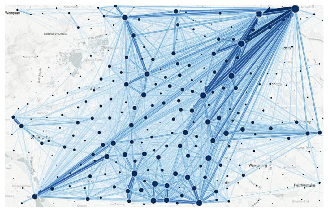
The distribution of the start points and end points of the trajectory is determined based on the OD survey. Traditional OD survey methods are varied and can capture the travel patterns of people, vehicles, and goods. Theoretically, an OD travel sample of a vehicle can generate a trajectory route under this OD constraint. During the process of trajectory data augmentation, if there are previously generated vehicle OD survey data, they can be directly used. We conduct an OD survey of the research area based on historical trajectory data to simulate the spatial allocation of trajectory data.

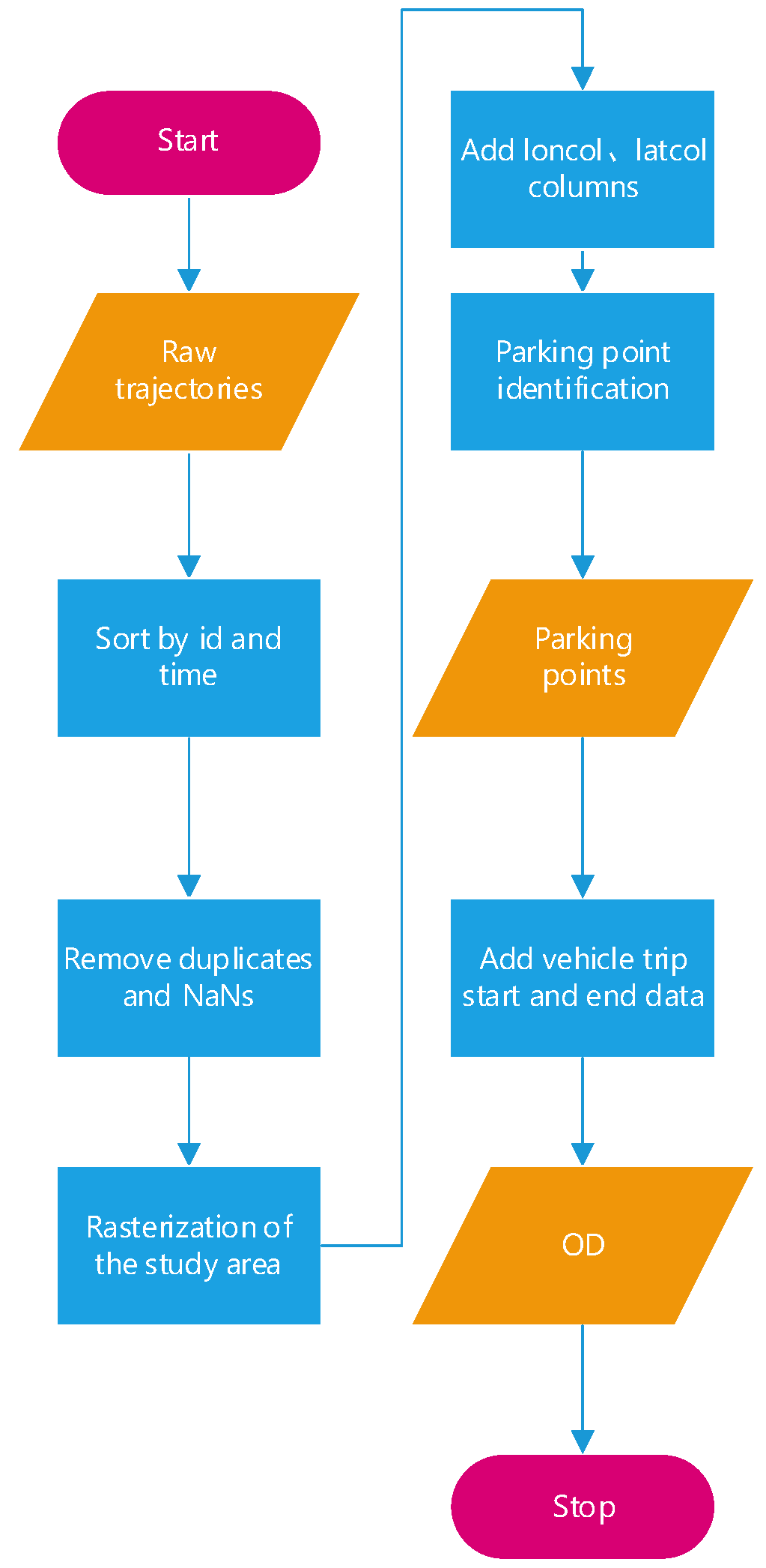
The main processing flow of OD information extraction is as shown in Figure 3. First, the raw trajectory dataset is input and sorted based on the vehicle acquisition times. Now the displacement points of each vehicle sorted by time can be obtained. Next, noise data caused by transmission errors or other issues are removed. The study area is then rasterized, and the rasterized grid information is assigned to each trajectory point. Rasterization helps to reduce positional deviation noise between trajectory points and the true locations. After adding the rasterized column information, the parking point information of each vehicle is extracted from the trajectory data based on the vehicle position change and the time interval threshold. The starting and ending travel information of the vehicle is added to the parking point information. And then, the segmented vehicle travel information is obtained, that is, how many times each vehicle travels in total within the study period and the starting and ending points of each trip. Furthermore, the OD statistical information of all vehicles is obtained. In this paper, the statistics of OD information are divided into the statistics of the start point, end point, and the combination of the two.

After completing the OD statistics of trajectories, the spatial allocation of trajectory data is realized by using this result. First, the allocation of the starting and ending points of the simulated trajectories is determined. In our research, the weighted random selection method is adopted to select the start point and end point for the trajectory, where each node is selected as the weight of the start point and end point, that is, the probability after OD statistics. Mathematically, the OD distribution is expressed as follows:

$$p_n={\displaystyle \frac{sum\left(n_s\right)}{sum}},$$

(7)

where $p_n$ represents the probability of node n as the start point, $sum\left(n_s\right)$ refers to the number of trajectories of node n as the start point obtained statistically, and sum is the total number of trajectories. Similarly, the weight of each node as the end point and each OD pairs can also be obtained.

When selecting OD points, the starting point or ending point is first selected based on their OD distribution, and then the other point is chosen according to the corresponding OD pairs statistics. Thereafter, each OD pair must exist in the real data, which avoids the situation where the starting point and end point are the same.

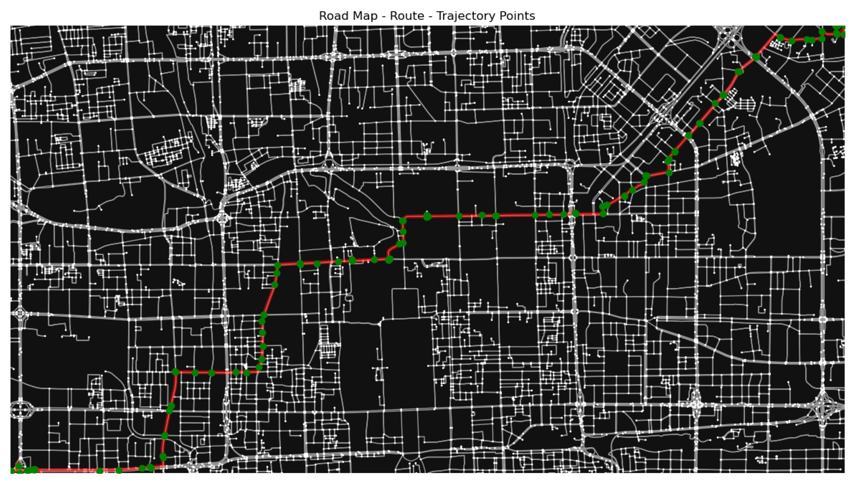
The OD information of the trajectory is matched to the node of the road map according to the principle of the shortest distance to determine the start and end nodes of the route. Then, under the given map and OD information, the entire route is obtained by using the shortest path (including the shortest time and the shortest space). This route is a list composed of several adjacent nodes in the road map.

Calculate Ideal Trajectory Point Positions

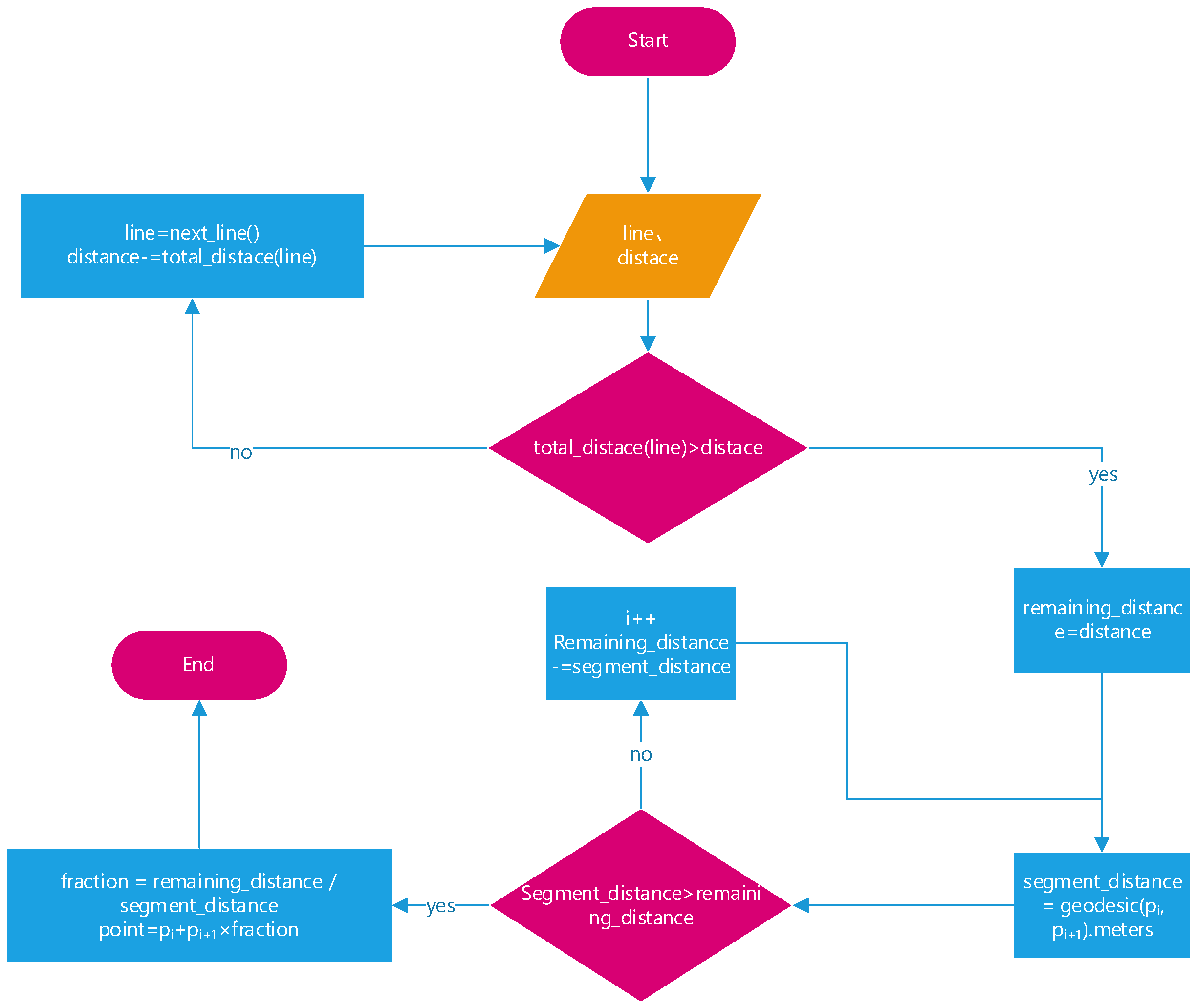
Each edge in the road map is associated with an inherent attribute: speed, which represents the recommended speed for a vehicle traveling along that edge. Starting from the origin, at each time interval, the expected position of the vehicle before it reaches the end of the edge can be determined by interpolating along the edge based on the distance traveled from the starting point, as follows:

$$\mathrm{d}\mathrm{i}\mathrm{s}\mathrm{t}\mathrm{a}\mathrm{n}\mathrm{c}\mathrm{e}={\mathrm{s}\mathrm{p}\mathrm{e}\mathrm{e}\mathrm{d}\_\mathrm{e}}_{\mathrm{i}}\times \mathrm{i}\mathrm{n}\mathrm{t}\mathrm{e}\mathrm{r}\mathrm{v}\mathrm{a}\mathrm{l}\times 1000/3600.$$

(8)

$$\mathrm{p}\mathrm{o}\mathrm{i}\mathrm{n}\mathrm{t}=\mathrm{e}\mathrm{d}\mathrm{g}\mathrm{e}.\mathrm{i}\mathrm{n}\mathrm{t}\mathrm{e}\mathrm{r}\mathrm{p}\mathrm{o}\mathrm{l}\mathrm{a}\mathrm{t}\mathrm{e}\left(\mathrm{d}\mathrm{i}\mathrm{s}\mathrm{t}\mathrm{a}\mathrm{n}\mathrm{c}\mathrm{e}\right).$$

(9)

The process of obtaining trajectory points by interpolation based on the driving distance on a road edge is as follows: Firstly, the total length of each edge is calculated by adding the geographical distance between each pair of adjacent coordinate points. The distance between two points is calculated using the geodesic function in the Geopy library based on the curvature of the Earth. Then, we determined the position of the vehicle on edge based on the distance it travels. The interpolation process is shown in Figure 4.

Introduce Noise into Trajectory Points

Trajectory point noise can be primarily classified into two types: transmission noise and positional offset noise. Transmission noise arises during the transmission process and includes three main types: repeated transmission of trajectory points, failed transmission of trajectory points, and delayed transmission of trajectory points. The effects and simulation methods associated with these three types of noise are summarized in

Table 2. Noise types and simulation methods.

Noise Type	Noise Effect	Simulation Method
Redundant Transmission	Trajectory contains identical trajectory data points	Select and duplicate trajectory data based on a certain probability
Trajectory point transmission failed	The trajectory points of a route do not follow the specified interval consecutively	Remove trajectory point data with a specified probability
Delay in transmitting trajectory points	The intervals between consecutive trajectory points of a route are not consistent in the specified interval	Introduce a 1–3 s deviation to the time attribute of trajectory points based on a certain probability

.

Positional offset noise refers to the deviation between the vehicle’s actual position and the positioning data, caused by limitations in the positioning technology. In our study, positional offset noise is simulated by adding Gaussian noise to the trajectory point positions. The mean and standard deviation (std) of the Gaussian noise are set according to simulation requirements, with adjustments made based on statistical data. The position calculation method after adding noise is shown in the following formulas.

$$\mathrm{noise}\_\mathrm{lon}=\mathrm{N}\mathrm{o}\mathrm{r}\mathrm{m}\mathrm{a}\mathrm{l}(mean,std).$$

(10)

noise_lat = Normal(mean,std).

(11)

lon = ideal_lon + noise_lon.

(12)

lat = ideal_lat + noise_lat.

(13)

3. Experimental Setup and Results

In this section, we validate the proposed trajectory augmentation method using real-world trajectory datasets. Spatiotemporal distribution features of traffic flow are extracted, and simulated trajectory data are generated based on the spatiotemporal characteristics of traffic volume. In our experiments, we use the T-Drive trajectory dataset to evaluate the effectiveness of our proposed methods [26,27]. This dataset contains one week’s worth of trajectory data from 10,357 taxis, with a total of approximately 15 million data points and a total trajectory distance of 9 million kilometers.

3.1. Extraction of Spatiotemporal Distribution Features

We performed a statistical analysis of the time distribution of the trajectory data in the dataset, categorized by day of the week and hour. The statistical results are shown in Figure 5. Based on the time distribution characteristics derived from the statistical analysis of T-Drive taxi trajectory data, it is observed that the number of travel routes on Monday is the highest, accounting for 0.2051. This might be because Monday marks the beginning of the working week, and many people have fixed travel needs such as going to work or school. The number of trajectories on Sundays is also relatively high, accounting for 0.1974. This discrepancy may be attributed to the fact that many people tend to travel on weekends for leisure activities, shopping, or visiting relatives.

Statistical analysis of the trajectory data by hour reveals that the peak travel period occurs primarily between 14:00 and 18:00, with a particularly notable peak from 16:00 to 17:00. This suggests that travel activities are closely tied to the start and end times of the typical working day. Although travel volume decreases at night, there is still notable activity between 20:00 and 23:00, indicating a continued demand for travel after dinner or during the evening hours. Travel is least frequent during the early morning hours, suggesting that most people are at rest during this time. These findings align with common daily routines and can provide valuable insights into simulating trajectory data.

The statistical results of the sampling interval of the T-Drive trajectory datasets are shown in Figure 6. The proportion of 300 s is the highest, approaching 19%. This suggests that in the data sampling process, intervals of 300 s account for a large proportion, with considerable volumes of data also observed at 301 and 302 s. Based on the noise characteristics of the trajectory data, this may be due to delays during data transmission when the vehicle’s sampling interval is set to 300 s. This insight is useful for understanding the noise patterns in the simulated trajectory data. From the distribution of sampling intervals, short time intervals (such as 1 s, 3 s, 5 s) and medium time intervals (such as 10 s, 30 s, 60 s) frequently occur in the data, indicating that the purpose of sampling is to capture relatively frequent changes. Sampling at longer time intervals (such as 300 s, 600 s) may be used to analyze data trends over a longer period.

After the travel identification of the trajectory data, the starting point and destination information of each travel can be obtained. The statistical results of the OD distribution of the T-Drive datasets are shown in Figure 7. After trip identification, all trajectory data were categorized into 191,070 trip records. According to the statistical results, the distribution of the starting point and the destination reveals the diversity of travel. The nodes with the highest number of start and destination distributions show a degree of repetition, indicating strong travel demand between these locations. These nodes are likely to be transportation hubs, such as railway stations or airports. Some combinations of starting and ending points occur only a few times, indicating that the mobility between these areas is relatively low. They may be places with inconvenient transportation or for special purposes of travel. The concentration of trajectories with specific Start and End Point combinations suggests distinct travel patterns in this area, such as a high volume of movement from office to residential areas, or from commercial zones to shopping centers.

As shown in Figure 8, the start and end points of taxi trajectories are visualized on the map, illustrating the distribution of vehicle travel points in the area. This visualization highlights key traffic flow hotspots, such as the city center, commercial districts, and transportation hubs, which typically exhibit a high density of starting and ending points.

3.2. Generation of Simulated Trajectory Data

After assigning OD pairs to each trajectory based on OD statistics, the driving route for the given OD can be determined using the route planning function of the multi-directional road map. The route is represented as a list of nodes traversed by the vehicle, where each element corresponds to the OSM ID of a node. In other words, for a given path, all the edges along the route can be identified. Using road edge data (including section length, suggested speed, etc.) and the intervals between collected trajectory points, all trajectory points along the path are generated, as shown in Figure 9.

Trajectory data is generated based on the current strategy. In addition to conventional trajectory information such as time, longitude, and latitude, additional auxiliary data can be incorporated based on application requirements. For instance, map-matching functionality can be implemented through machine learning. The generated trajectory data consists of five columns: time, lon, lat, moveid, edge_u, and edge_v, as shown in

Table 3. Sample of augmented trajectory data.

Time	Lat	Lon	Moveid	edge_u	edge_v
14 April 2025 00:00:00	116.507	40.011	0	1736475374	1736475373
14 April 2025 00:00:15	116.508	40.010	0	1736475373	353122060
14 April 2025 00:00:30	116.516	40.015	0	353122060	2377580202
14 April 2025 00:00:45	116.517	40.015	0	353122060	2377580202
14 April 2025 00:00:59	116.517	40.014	0	353122060	2377580202

. These columns represent the timestamp, location, travel ID, and the start and end points of the road edge associated with each trajectory point. The road edge information in the trajectory data is used for model training.

3.3. Comparison Between Simulated Trajectory and True Trajectory

We conducted a comparative analysis of the similarity between the generated trajectory data and the real trajectory dataset in terms of both time and spatial distributions. For the time distribution of trajectory data, at a macro level, we rely on the statistical distribution probability proportion. We multiply the total number of desired generated trajectory data by this proportion to determine the number of trajectories for each day. Then, for each hour, we allocate the number of trajectories based on the historical data distribution ratio for each hour on each weekday. The proportion of the simulated trajectory data and the real trajectory data in both the daily and hourly units are evidently identical, as confirmed by the experimental results, which will not be presented here.

Within each hour, we use the Poisson distribution to determine the departure time of each trajectory. To analyze the distribution of trajectories on a minute-by-minute basis, we calculated the minute-level distribution probability of trajectory data within each hour and selected data from one specific hour for illustration. Figure 10 shows the distribution proportion of real and simulated trajectory data for each minute within the same hour. We further compared these statistical results using the Kolmogorov–Smirnov (K-S) test, a commonly used method for comparing distributions, which effectively evaluates the similarity between the distributions of simulated and real trajectory data.

Based on the K-S test results shown in Figure 10, the distribution of simulated trajectory data and real trajectory data in terms of time is highly similar. The K-S test D value is 0.133, indicating that the distribution difference between the two is small. The p-value of 0.665 suggests that we cannot reject the null hypothesis, meaning that the simulated data can effectively mimic the time distribution of the real trajectory data.

For the OD distribution of trajectory data, we simulate it using a random distribution based on the OD weight from historical trajectory data. We then perform statistical analysis on the OD distribution of the real and simulated trajectory data. The top 20 OD pairs (10 origin nodes and 10 destination nodes) with the highest data proportion are selected, and we compare their distributions using the Kolmogorov–Smirnov (K-S) test.

As shown in Figure 11, the K-S test D value is 0.3, indicating a small distribution difference between the two datasets. The p-value is 0.787, suggesting that the simulated data can effectively replicate the OD distribution of the real trajectory data.

To validate the spatial distribution consistency between the simulated trajectory points and the real trajectory points, we compare the spatial distribution and relative distances of simulated and real trajectories with the same OD pairs.

First, the OD of the real trajectory is extracted, and the nearest map node to these points is selected as the OD of the simulated trajectory. Then, the trajectory generation method mentioned earlier is used to simulate the trajectory, which is compared with the real trajectory, as shown in Figure 12. From the “Comparison of Spatial Positions” results, it can be seen that the simulated trajectory exhibits overall spatial consistency with the real trajectory, indicating that the path planning and trajectory point generation methods of the simulated trajectory can effectively replicate real driving behavior. However, there are differences in the spatial distribution between the simulated and real trajectories, suggesting that relying solely on recommended speeds for road segments to predict vehicle positions has certain limitations. In real life, drivers usually adjust their speed based on real-time traffic conditions, congestion, speed limit enforcement, and other factors. Additionally, from the time–distance variations, the simulated trajectory points show a generally linear increase in distance from the starting point on each road segment, while the real trajectory points exhibit phase-based changes. On some segments, the distance between the trajectory points and the starting point changes more slowly, indicating potential congestion on that segment, whereas on other segments, the distance changes more rapidly, suggesting smoother traffic flow. These features are highly consistent with actual traffic conditions.

4. Discussion

We approach the problem of trajectory augmentation from a macroscopic perspective by generating simulated trajectory data based on historical trajectory information. By extracting spatiotemporal traffic flow characteristics and road network from the historical data, we are able to simulate realistic vehicle movement patterns that capture the temporal and spatial dependencies of real-world traffic dynamics. By leveraging road network information alongside spatiotemporal traffic patterns, the generated simulated trajectories can more accurately reflect the movement of vehicles of target environments. One of the key advantages of our approach is its ability to generate accurate classification information for training machine learning models under different traffic conditions.

The trajectory data generation method proposed in this paper is well suited for simulating the overall traffic flow distribution in urban environments. It focuses on modeling the global distribution of traffic and ensures accurate matching of trajectory points with the underlying map. By incorporating spatial and temporal patterns of traffic movement, the method not only simulates traffic flow but also aligns the generated trajectories with real-world infrastructure and road networks. This approach is essential for large-scale urban traffic simulations, as it captures both the macro-level traffic patterns and the precise interactions between trajectory points and the map, enabling more realistic and effective traffic management strategies. However, it does have certain limitations, as it lacks the simulation of individual vehicle path choice diversity, the random behavior of drivers during the driving process, and the real-time fluctuations in traffic flow. These aspects, which are critical for capturing the detailed variability in traffic behavior, are not fully addressed in this approach.

Furthermore, some improvements are needed in our method. Firstly, during the generation of simulated trajectory data, factors such as the interaction between vehicles, individual driving habits, and unexpected events were not considered in the trajectory simulation. Secondly, the generation of trajectory data is based on the traffic flow characteristics derived from historical trajectory data. However, in real-world situations, historical trajectory data is often collected from a subset of probe vehicles, which may not fully reflect the traffic flow characteristics of a specific area.

5. Conclusions

In this paper, we explore the generation of synthetic trajectory data by leveraging the spatiotemporal distribution characteristics of traffic flow, as well as road map and segment features. First, we extract the temporal distribution from historical trajectories. Then, we use the Poisson distribution to determine the starting time for each trajectory and apply the OD distribution to define the start and end positions. Next, we utilize road map and edge characteristics to generate subsequent trajectory points. Additionally, we introduce a trajectory noise simulation module to account for both spatial and temporal noise in the trajectory points. Extensive experiments on a real-world trajectory dataset demonstrate that our method can effectively generate useful synthetic trajectory data. This work represents a preliminary attempt to address the trajectory augmentation problem by utilizing spatiotemporal distribution characteristics of traffic flow and road map. It enables the generation of trajectory data enriched with additional confirmed information, making it particularly valuable for learning-based research.

In our future work, we intend to develop a machine learning model aimed at enhancing the accuracy and reliability of the generated trajectory data. The model will focus on better estimating the trajectories by considering various contextual factors, such as traffic patterns and driver behavior, to improve prediction accuracy. Additionally, we plan to explore the use of deep learning techniques, such as recurrent neural networks or long short-term memory networks, which are well suited for time-series data, to capture the temporal dependencies in trajectory patterns. In addition, we plan to apply the proposed method to generate simulation trajectory data, which will then be utilized in learning-based map matching applications. This will allow us to explore the integration of the generated data with advanced machine learning techniques for improving the accuracy and efficiency of map matching processes in real-world traffic systems.