EL-GNN: A Continual-Learning-Based Graph Neural Network for Task-Incremental Intrusion Detection Systems

Abstract

Modern network infrastructures have significantly improved global connectivity while simultaneously escalating network security challenges as sophisticated cyberattacks increasingly target vital systems. Intrusion Detection Systems (IDSs) play a crucial role in identifying and mitigating these threats, and recent advances in machine-learning-based IDSs have shown promise in detecting evolving attack patterns. Notably, IDSs employing Graph Neural Networks (GNNs) have proven effective at modeling the dynamics of network traffic and internal interactions. However, these systems suffer from Catastrophic Forgetting (CF), where the incorporation of new attack patterns leads to the loss of previously acquired knowledge. This limits their adaptability and effectiveness in evolving network environments. In this study, we introduce the Elastic Graph Neural Network for Intrusion Detection Systems (EL-GNNs), a novel approach designed to enhance the continual learning (CL) capabilities of GNN-based IDSs. This approach enhances the performance of the GNN-based Intrusion Detection System (IDS) by significantly improving its capability to preserve previously learned knowledge from past cyber threats while simultaneously enabling it to effectively adapt and respond to newly emerging attack patterns in dynamic and evolving network environments. Experimental evaluations on trusted datasets across multiple task scenarios demonstrate that our method outperforms existing approaches in terms of accuracy and F1-score, effectively addressing CF and enhancing adaptability in detecting new network attacks.

1. Introduction

As network technologies continue to advance, the expansion in connectivity has been paralleled by a notable increase in network attacks. This escalation in malicious activity has underscored the need for robust defense mechanisms, leading to the widespread adoption of Intrusion Detection Systems (IDSs) and Intrusion Prevention Systems (IPSs) to secure digital infrastructures [1]. Network Intrusion Detection Systems (NIDSs), one of the categories in IDSs, are specialized systems designed to monitor network traffic and system activities for signs of unauthorized or anomalous behaviors. NIDSs are broadly classified into two types: signature-based IDSs, which rely on established attack signatures to detect known threats, and anomaly-based IDSs, which identify deviations from normal behavior to flag potential novel attacks [2], as shown in Figure 1. In the context of rapidly evolving threats, traditional rule-based methods of detection have shown limitations in adaptability and responsiveness, thereby motivating the integration of machine learning techniques into IDSs [3]. By dynamically learning from new attack patterns and network behaviors, machine learning approaches empower IDSs to maintain a proactive stance against sophisticated network threats, ensuring an evolving defense that can keep pace with the rapid changes in both technology and adversarial methodologies [4]. Consequently, as network infrastructures grow more complex and the nature of threats becomes increasingly multifaceted, the advancement of IDSs through continuous learning and adaptive algorithms stands as a critical frontier in modern network security research and practice.

In recent years, Machine-Learning-based Network Intrusion Detection Systems (ML-based IDSs) have gained significant traction by leveraging advanced deep learning architectures to enhance threat detection capabilities [5]. Researchers have actively utilized techniques like Convolutional Neural Networks (CNNs) [6] to automatically extract spatial features directly from raw network traffic data. By learning hierarchical representations of the input, CNNs are able to identify intricate and non-linear patterns that are often associated with malicious behaviors, thereby enhancing the accuracy and efficiency of intrusion detection systems in recognizing sophisticated cyberattacks, while Recurrent Neural Networks (RNNs) [7] have been adept at capturing temporal dependencies inherent in sequential network communication. Other deep learning approaches, including autoencoders and hybrid models, have further contributed to the evolution of IDSs by enabling unsupervised anomaly detection and fine-grained behavioral analysis [8]. Despite these advancements, these systems often encounter limitations such as overfitting to specific datasets, an over-reliance on large amounts of labeled data, and challenges related to scalability and real-time implementation. Moreover, issues like vulnerability to adversarial attacks and interpretability remain persistent challenges [9]. Nonetheless, deep-learning-based IDSs have shown considerable promise, demonstrating superior capability in detecting sophisticated intrusions through automated feature extraction and dynamic modeling of network behaviors, thereby providing a robust foundation for evolving network defenses.

Graph Neural Networks (GNNs) represent an emerging class of deep learning models specifically engineered to process data structured in graph form. By leveraging node, edge, and overall graph topology information, GNNs are inherently capable of capturing intricate relational dependencies and inter-connectivity patterns [10]. This property is particularly advantageous for IDSs, where the complex interrelations of network entities naturally form graph structures—representing communication links, traffic flows, and behavioral interactions. In the context of IDSs, GNNs facilitate the transformation of raw network data into graphs that model the inherent structure of network traffic, enabling the detection of anomalous patterns that may be indicative of malicious activities [11]. Their ability to effectively process both local and global graph features makes them well suited for identifying coordinated or distributed attacks, which often manifest through subtle yet consistent relational dynamics [12].

As adversaries continue to innovate, IDSs must be updated continually to adapt to emerging threats. Traditional GNN-based IDS approaches [13,14,15,16] that retrain models from scratch with each new attack pattern are computationally burdensome and time-intensive. However, this shift introduces the phenomenon known as Catastrophic Forgetting (CF) [17], wherein a model, while learning new information, inadvertently loses or overwrites critical knowledge about previously encountered threats [18]. In the context of GNN-based IDSs [19], which rely on capturing intricate relational and structural patterns within network data, CF can severely undermine detection capabilities. As the system evolves to incorporate information about new attack vectors, the degradation of earlier learned representations may lead to diminished performance on known malicious behaviors, ultimately weakening the overall resilience of the IDS [20].

Continual learning (CL) [21], also known as incremental or lifelong learning, refers to the ability of a system to learn from a sequential stream of data, adapting to new tasks and information while preserving previously acquired knowledge. This methodology directly addresses the challenge of CF and architectural adjustments that selectively consolidate prior knowledge with new data [22]. In the domain of IDSs, where evolving network attack vectors and dynamic network behaviors necessitate frequent updates to the detection model, CL offers a promising solution. By incrementally updating the system rather than retraining from scratch, CL minimizes computational overhead and reduces downtime while ensuring that the IDS retains its effectiveness against both known and emerging threats [23,24]. Consequently, integrating CL into GNN-based IDSs is particularly beneficial as it allows the system to adapt to new network structures and attack patterns without compromising the detection accuracy built on historical data.

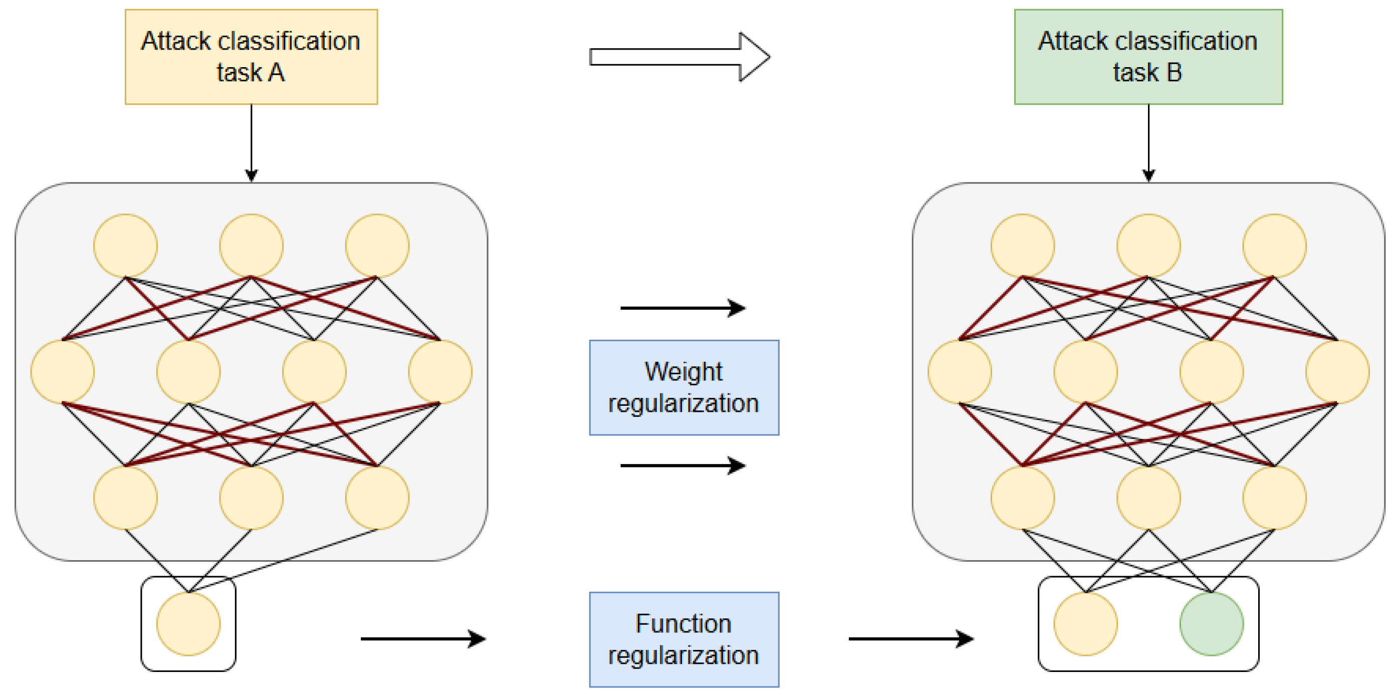
In this publication, we introduce the EL-GNN, a novel framework that we developed by integrating two foundational approaches: the representational power of Graph Convolutional Networks (GCNs) plus the stability-focused weight regularization strategy commonly used in continual learning (CL) techniques. By combining these methodologies, our proposed model leverages the structural learning capabilities of GCNs while incorporating a penalty-based mechanism to preserve important parameters, effectively addressing the challenge of catastrophic forgetting in dynamic intrusion detection scenarios. As described in Figure 2, CL’s weight penalty methods measure the importance of each weight in the network, reserve the important weights in the network, and penalize the weights that have less importance. Additionally, we applied the model to the Canadian Institute for Cybersecurity (CIC-IDS-2017) and University of New South Wales (UNSW-NB15) datasets. The experimental findings demonstrate that the following results reduce the impact of CF while also proving the effectiveness of the model in single-task training.

The key contributions of our work can be comprehensively outlined as follows:

• We proposed the EL-GNN, a method that leverages GNN-based IDSs combined with the adaptability of CL methods.
• The proposed method significantly reduces CF on GNN-based IDSs, thereby improving the model’s ability to learn continuously in dynamic environments.
• The proposed method demonstrates the effectiveness of GNN-based intrusion detection systems in single-task training scenarios.
• Using standardized datasets, the proposed method demonstrates strong performance and reliability, providing confidence in its effectiveness for CL in IDSs.

The organization of this paper is structured to guide the reader through the progression of our research in a logical and coherent manner. Section 2 presents a comprehensive review of the existing literature and closely related work, highlighting the current state of research in intrusion detection systems and graph-based learning approaches. In Section 3, we lay the necessary theoretical groundwork by providing an in-depth overview of the IDS and GNN, which form the basis for our proposed methodology. Section 4 is dedicated to a detailed explanation of the proposed EL-GNN model, including its architectural design, core components, and the motivation behind its development. Section 5 outlines the experimental framework used to evaluate the effectiveness of the model, including descriptions of the datasets, evaluation metrics, and implementation details. Lastly, Section 6 concludes the paper by summarizing the key findings of our study, addressing its current limitations, and offering insightful recommendations for future research directions in this domain.

2. Related Works

In this section, we conduct a comprehensive review of recent studies related to GNN-based IDS and CL-based IDS models. These studies represent the most advanced approaches currently available for leveraging GNN-based models to analyze and predict network traffic patterns. Some of these models specifically focus on mitigating the challenge of CF, which is a critical issue in CL frameworks. By examining these prior works, we aim to provide an in-depth understanding of the strengths and limitations of existing methodologies. Additionally, we highlight the distinctions between these studies in terms of their proposed methods, underlying architectures, and strategies for improving model performance in dynamic network environments. This analysis serves as a foundation for positioning our proposed approach within the context of existing research and identifying key areas for further improvement.

Recent research into the IDS highlights the adoption of deep learning techniques, though limitations in traditional approaches underscore the need for GNN-based methods. Studies employing CNN and RNN demonstrate competitive performance but face critical constraints. For instance, a comparative analysis of Deep Belief Networks (DBNs), CNNs, Long-Short Term Memory (LSTM), and LSTM-RNNs found CNNs achieved promising accuracy, yet all models processed flows independently, ignoring network topology [25]. Hybrid architectures like CNN-LSTM improved feature extraction through spatial–temporal analysis but remained vulnerable to adversarial perturbations altering packet features [26]. Similarly, a CNN-BiLSTM model with Principal Component Analysis (PCA) achieved high accuracy on CIC-IDS-2017 but struggled with multi-flow attack patterns due to isolated flow analysis [27]. These approaches inherently lack structural awareness, rendering them ineffective against coordinated attacks (e.g., Distribution Denial of Service (DDoS)).

GNNs have emerged as a powerful approach, offering not only the capability to effectively represent network flow data as graphs but also the ability to capture complex relationships, making them highly suitable for the IDS. Previous studies have demonstrated significant success in leveraging GNNs within the IDS domain. For instance, the work in [28] introduced E-GraphSAGE and E-ResGAT, two widely recognized models that utilize Graph Sample and Aggregate (GraphSAGE) and Graph Attention Network (GAT) as their backbone and incorporate edge detection techniques for IoT networks. This research provides a novel perspective on the role of edge processing in network flow graphs. Similarly, the study in [29] proposed a system based on the GCN, a deep learning framework capable of capturing both the topological and statistical relationships between attack networks and victim networks.

Another notable study presented in [30] introduced a graph-based intrusion detection model that effectively integrates Graph Convolutional Networks (GCNs) with Sample Aggregation and Convolutional (SAGEConv) layers, which are a variant of the GraphSAGE architecture. This hybrid design leverages the strengths of both the GCN and GraphSAGE to enhance representational learning over complex network structures. In this model, graph nodes are initialized using features derived from network flow data, allowing the system to encode rich behavioral information associated with individual traffic flows. Meanwhile, graph edges are constructed by analyzing the relationships between IP addresses, capturing the underlying communication patterns and structural dependencies present within the network. By combining flow-level semantics with IP-level topology, this approach significantly improves the model’s ability to detect anomalous or malicious activity, thereby advancing the overall effectiveness of network intrusion detection systems. Additionally, the research in [31] introduced ARGANIDS, a model based on the Adversarially Regularized Graph Autoencoder (ARGA) algorithm. This method improves robustness by incorporating an adversarial regularization phase, enabling it to outperform other state-of-the-art GNN-based approaches in NIDSs.

Despite these advancements, existing models share a critical limitation. Since NIDSs must continuously adapt to emerging network attack threats, they require incremental updates to incorporate newly identified attacks. However, conventional GNN-based approaches struggle with CF, where learning new attack patterns leads to the unintentional loss of previously acquired knowledge.

One notable work presented Semi-supervised Privacy-preserving Intrusion Detection with Drift-aware CL (SPIDER) [32], a novel approach designed to manage CL effectively without the need to store labeled samples from all previous tasks. SPIDER integrates Gradient Projection Memory (GPM) with Self-Supervised CL (SSCL) to mitigate CF while maintaining model performance. This method demonstrated competitive results compared to fully supervised and semi-supervised baseline models, achieving comparable accuracy while requiring only up to 20% of annotated data. Moreover, SPIDER significantly optimized training efficiency, reducing the total training time by a factor of two. This highlights its potential for real-world deployment, where both data privacy concerns and computational constraints pose major challenges for IDSs. Another significant contribution in the field extended Class Balancing Reservoir Sampling (ECBRS) [33], a memory-based CL strategy, to specifically tackle the issue of class imbalance in large-scale datasets. Traditional CL models often struggle with imbalanced data distributions, leading to biased model updates and degraded performance over time. To address this, the study also proposed Perturbation Assistance for Parameter Approximation (PAPA), an innovative approach based on the Gaussian Mixture Model (GMM). PAPA effectively reduces the computational overhead associated with virtual Stochastic Gradient Descent (SGD) updates by strategically identifying and prioritizing maximally interfering samples. By lowering the number of virtual SGD update operations, PAPA leads to substantial improvements in training efficiency, with reported reductions in training time ranging between 12% and 40% compared to conventional maximally interfered sample retrieval algorithms. Furthermore, Gradient Episodic Memory (GEM) [34] has been widely adopted as a memory-based CL method that explicitly stores a subset of previous task data and projects current gradients to prevent interference. GEM serves as a foundational technique for rehearsal-based methods, enabling continual learning in IDSs while maintaining high accuracy and controlling forgetting across task boundaries.

Table 1. Structured comparison of continual learning models.

Feature	SPIDER [32]	ECBRS [33]	PAPA [33]	GEM [34]
Key Characteristics	Dynamic sparse MLP + replay	Episodic encoder–decoder	Prototype-based pseudo-replay	Gradient memory constraints
Performance	Strong in low-resource settings	Moderate, fast adaptation	Competitive on stream data	High on standard CL benchmarks
Advantages	Memory-efficient and adaptive	Low compute cost	Simple and fast adaptation	Effective CF prevention
Limitations	Requires task boundaries	Lacks deep structural modeling	Sensitive to prototype drift	Computationally expensive
CF Mitigation Strategy	Replay with sparse updates	Episodic replay	Prototype-based pseudo-memory	Gradient projection constraints

below shows the comparison of continual learning model that are related to our works.

These advancements mark significant progress in developing more efficient and scalable CL methods for IDSs, addressing key challenges such as CF, class imbalance, and computational efficiency. However, despite these improvements, further research is still required to enhance adaptability in dynamic network environments and ensure robustness against evolving network attack threats. Unlike previous studies that address either relational modeling or catastrophic forgetting in isolation, our method combines the strengths of both GNN-based relational learning and continual learning techniques. This integrated approach enhances the model’s robustness, effectiveness, and adaptability within dynamic IDS environments.

3. Background

3.1. Graph Neural Network

The GNN was originally proposed in 2009 in [35] by Franco Scarselli, aimed to develop a neural network model capable of learning from GNN-based data, which is common in real-world applications such as social networks, molecular structures, and knowledge graphs. Traditional neural networks struggle with irregular, non-Euclidean data, limiting their applicability to GNN-based problems. By introducing a framework where nodes iteratively update their states based on neighboring information, GNNs enable efficient learning and representation of graph structures. By leveraging message passing, GNNs aggregate information from neighboring nodes, enabling effective analysis of network structures in applications like fraud detection, recommendation systems, and intrusion detection. Their ability to model both local and global dependencies makes GNNs a powerful alternative to CNNs and RNNs for GNN-based problems. GNNs operate by leveraging a message-passing mechanism to learn from graph-structured data, where nodes represent entities and edges capture their relationships. The core idea of GNNs, as shown in Figure 3, is to iteratively update node representations by aggregating information from their neighbors, allowing the model to capture both local and global structural dependencies. This process consists of three key steps: message passing, aggregation, and update.

In the message-passing phase, each node collects information from its adjacent nodes. The aggregation step then combines these messages using techniques such as mean, sum, or attention-based weighting. Finally, in the update phase, the node’s representation is refined based on the aggregated information. This iterative process continues for multiple layers, enabling nodes to incorporate information from progressively distant neighbors. The final node embeddings can then be used for various tasks such as node classification, link prediction, and graph classification. GNNs are widely used in applications like fraud detection, molecular analysis, and intrusion detection, where capturing relational dependencies is essential for accurate predictions.

3.2. Graph Convolutional Network

The GCN [36] is a fundamental model in GNN, designed to efficiently process graph-structured data. Inspired by CNNs, which extract spatial features from grid-structured data such as images, GCNs extend this concept to non-Euclidean domains, where data points (nodes) are interconnected in arbitrary structures. The key idea behind GCNs is to aggregate information from neighboring nodes in a systematic way, allowing each node’s representation to be updated based on the features of its local graph structure. This makes GCNs particularly well suited for tasks such as node classification, link prediction, and graph classification, where capturing the relationships between entities is crucial.

A GCN operates on an input graph consisting of nodes, edges, and an associated feature matrix. Each node starts with an initial feature vector, which is iteratively refined through multiple layers of the network. Each GCN layer performs a message-passing operation, where nodes aggregate information from their immediate neighbors, transforming their feature representations. This process is mathematically formulated as follows:

$$H^{(l+1)}=\sigma ({\tilde{D}}^{-\frac{1}{2}}\tilde{A}{\tilde{D}}^{-\frac{1}{2}}{H}^{\left(l\right)}{W}^{\left(l\right)})$$

(1)

where $\tilde{A}$ is the adjacency matrix with self-loops added, $\tilde{D}$ is the corresponding degree matrix, $W^{\left(l\right)}$ is the learnable weight matrix, $H^{\left(l\right)}$ represents the node feature matrix at layer l, and $\sigma$ is a non-linear activation function (typically ReLU). This operation normalizes and propagates information through the graph while maintaining stability in the learning process.

Through multiple layers, nodes accumulate information from progressively larger neighborhoods, enabling the model to capture both local and global graph structures. The final layer of the model generates task-specific embeddings that capture meaningful representations tailored to the learning objective. These embeddings can be effectively utilized in various downstream applications, such as semi-supervised node classification—where only a limited subset of nodes is labeled and the goal is to infer labels for the remaining nodes—and graph classification, where the model assigns a categorical label to an entire graph based on its overall structure and features. Compared to other GNN architectures, GCNs provide an efficient, scalable, and interpretable approach to learning from graph-structured data, making them a foundational model in GNN-based deep learning.

3.3. Catastrophic Forgetting

CF, also known as catastrophic interference, was first identified by McCloskey and Cohen (1989). As shown in Figure 4, it was observed that when deep learning models are trained on new tasks, they tend to lose knowledge acquired from previously learned tasks. This occurs because the optimization process updates the model’s weights to adapt to the new task, inadvertently overwriting information from earlier tasks and leading to performance degradation. Without addressing this issue, neural networks would struggle to retain knowledge while learning new tasks. Abraham and Robins referred to this challenge as the stability–plasticity dilemma, where a highly stable model resists learning new information, while a highly plastic model undergoes substantial weight modifications, causing it to forget prior knowledge. Thus, achieving an optimal balance between stability and plasticity is crucial for ensuring that neural networks can continuously learn without forgetting past experiences.

CF presents a significant challenge for GNN-based IDSs, particularly in dynamic network environments where cyber threats continuously evolve. These systems rely on GNNs to model network structures and detect anomalies based on relationships between entities. However, when trained incrementally on new attack patterns, GNN-based IDSs risk forgetting previously learned intrusion signatures, leading to reduced detection accuracy for past threats. This phenomenon occurs due to the sequential nature of training, where updated model parameters overwrite earlier learned representations, thereby compromising the system’s ability to recognize recurring or modified attack vectors.

The implications of CF in GNN-based IDSs are profound as cybersecurity threats often exhibit repetitive and evolving characteristics. An IDS that fails to retain historical attack knowledge may struggle to detect reoccurring threats, particularly those that manifest with slight modifications. Furthermore, network environments are inherently dynamic, with new nodes, connections, and threat patterns emerging over time. This necessitates an optimal balance between stability and plasticity, where the system remains adaptive to new threats without compromising its ability to detect previously known intrusions. Addressing CF in GNN-based IDSs is, therefore, crucial for enhancing long-term detection performance and ensuring robust, real-time network security.

3.4. Continual Learning

CL or lifelong learning [37] is a machine learning paradigm that enables models to learn sequentially from a stream of tasks while retaining previously acquired knowledge. Unlike traditional machine learning approaches, which assume access to a fixed dataset, CL aims to develop models that adapt to new information without forgetting past knowledge. The concept of CL has its origins in cognitive science, where human learning is recognized as a continuous process of accumulating and refining knowledge over time. Various methodologies have been proposed, broadly categorized into regularization-based methods, replay-based methods, and architectural approaches.

In this work, we focus on exploring regularization-based methods, which aim to address CF by preserving knowledge from previous tasks while allowing adaptation to new ones. Unlike replay-based approaches that store past data, regularization-based methods introduce penalties in the loss function to constrain changes in model parameters, ensuring that critical information is retained. These methods estimate the importance of each parameter and prevent significant modifications to those that contribute substantially to past tasks. Three prominent regularization-based approaches are Elastic Weight Consolidation (EWC) [38], Synaptic Intelligence (SI) [39], and Memory Aware Synapses (MAS) [40], each employing distinct strategies to mitigate forgetting.

EWC, as shown in Figure 5, is one of the earliest and most widely adopted regularization-based CL techniques. It leverages the Fisher Information Matrix (FIM) to estimate the importance of each parameter based on how much it influences the previous tasks’ loss. During training on a new task, EWC adds a quadratic penalty to the loss function, discouraging large changes to critical parameters:

$${\mathcal{L}}_{EWC}=\mathcal{L}+{\displaystyle \frac{\lambda }{2}}\sum _i{F}_i{({\theta }_i-{\theta }_i^{*})}^2$$

(2)

where,

$F_i$

: Fisher Information Matrix.

${\theta }_i$

: optimal parameters from current tasks.

${\theta }_i^{*}$

: optimal parameters from previous tasks.

$\lambda$

: the balance between past and new learning.

By anchoring the most influential parameters, EWC allows learning of new tasks while minimizing interference with previously acquired knowledge.

SI builds upon EWC but takes a different approach to estimating parameter importance dynamically during training. Instead of relying on the Fisher Information Matrix, SI tracks the path integral of parameter changes over time, measuring how much each weight contributes to reducing the loss. The regularization term for SI is defined as

$${\mathcal{L}}_{SI}=\mathcal{L}+{\displaystyle \frac{\lambda }{2}}\sum _i{\Omega }_i{({\theta }_i-{\theta }_i^{*})}^2$$

(3)

where ${\Omega }_i$ represents the importance measure of parameter ${\theta }_i$, computed as

$${\Omega }_i=\sum _t{\displaystyle \frac{\Delta {\theta }_i^t{g}_i^t}{{(\Delta {\theta }_i^t)}^2+\xi }}$$

(4)

where,

$g_i^t$

: the gradient at time step t.

$\Delta {\theta }_i^t$

: the change in parameter.

${\theta }_i,\xi$

: a small constant to prevent division by zero.

Unlike EWC, SI continuously updates the importance weights throughout training, leading to a more flexible adaptation mechanism.

MAS introduces a novel approach to estimating parameter importance in an unsupervised manner. Unlike EWC and SI, which rely on task-specific losses, MAS measures the sensitivity of the model’s output to changes in parameters, making it task-agnostic. The importance of parameter ${\theta }_i$ is estimated as follows:

$${\Omega }_i={\mathbb{E}}_x{\left[{\displaystyle \frac{\partial f\left(x\right)}{\partial {\theta }_i}}\right]}^2$$

(5)

where,

${\Omega }_i$

: quantifies how much parameter.

${\theta }_i$

: influences the output $f\left(x\right)$ across different inputs x.

The MAS regularization loss is then

$${\mathcal{L}}_{MAS}=\mathcal{L}+{\displaystyle \frac{\lambda }{2}}\sum _i{\Omega }_i{({\theta }_i-{\theta }_i^{*})}^2$$

(6)

MAS is particularly effective in unsupervised and online learning settings since it does not require labeled data to compute importance. This makes it well suited for applications such as GNN-based IDSs, where network structures evolve over time and labeled attack patterns may be limited.

3.5. Pearson Correlation Coefficient

The Pearson Correlation Coefficient (PCC) [41], often denoted as r, is a widely used statistical measure that quantifies the linear relationship between two continuous variables. Introduced by Karl Pearson in the early 20th century, PCC evaluates how strongly the variations in one variable are associated with variations in another. The correlation coefficient takes on values between −1 and +1. A value of +1 denotes a perfect positive linear relationship between the two variables, while −1 represents a perfect negative linear relationship. A coefficient of 0 indicates the absence of any linear correlation. Mathematically, it is defined as the covariance between the two variables divided by the product of their standard deviations. PCC is particularly valuable in various fields such as machine learning, signal processing, and data analysis, where understanding linear dependencies between features or observations is crucial. However, it is sensitive to outliers and only captures linear associations, making it less effective in cases involving nonlinear relationships.

$$r={\displaystyle \frac{\sum (x_i-\overline{x})(y_i-\overline{y})}{\sqrt{\sum {(x_i-\overline{x})}^2\sum {(y_i-\overline{y})}^2}}}$$

(7)

where,

r 

: Pearson Correlation Coefficient.

$x_i$

: x variable samples.

$y_i$

: y variable sample.

$\overline{x}$

: mean of values in x variable.

$\overline{y}$

: mean of values in y variable.

3.6. Dataset

3.6.1. CIC-IDS-2017

The CIC-IDS-2017 dataset is a widely recognized benchmark for evaluating IDSs in cybersecurity research. It was designed to reflect real-world network traffic scenarios, capturing both normal and malicious activities to provide a comprehensive dataset for machine-learning-based intrusion detection. The dataset was generated using a realistic testbed environment that simulated various network behaviors, including legitimate user activities as well as different types of cyberattacks.

A key strength of CIC-IDS-2017 is its rich feature set, which includes more than 80 network traffic features extracted using Bro-IDS (now Zeek). These features capture essential characteristics of network flows, such as packet inter-arrival time, flow duration, protocol-specific behaviors, and statistical properties of transmitted data, allowing for in-depth analysis and detection of anomalies. The dataset encompasses a diverse range of attack types, including DDoS, brute-force attacks, botnet infections, web-based exploits, SQL injection, infiltration attacks, and port scanning, making it suitable for assessing the effectiveness of various IDS models.

3.6.2. UNSW-NB15

The UNSW-NB15 dataset is a widely used benchmark dataset for evaluating IDSs. It was designed to address the limitations of older datasets, such as KDD99 and NSL-KDD, by incorporating modern attack scenarios and real-world network traffic characteristics. The dataset was generated using the IXIA PerfectStorm tool, which emulates contemporary network traffic, including both normal and malicious activities, within a controlled testbed environment. This ensures that UNSW-NB15 better represents the complexity of modern cyber threats. A distinctive feature of UNSW-NB15 is its comprehensive set of 49 network traffic features, categorized into flow-based, content-based, time-based, and additional general network properties.

4. Proposed Methods

This section provides a comprehensive overview of our proposed model framework. We aim to systematically visualize and analyze the workflow underlying our approach. The following subsections detail the techniques incorporated in our method.

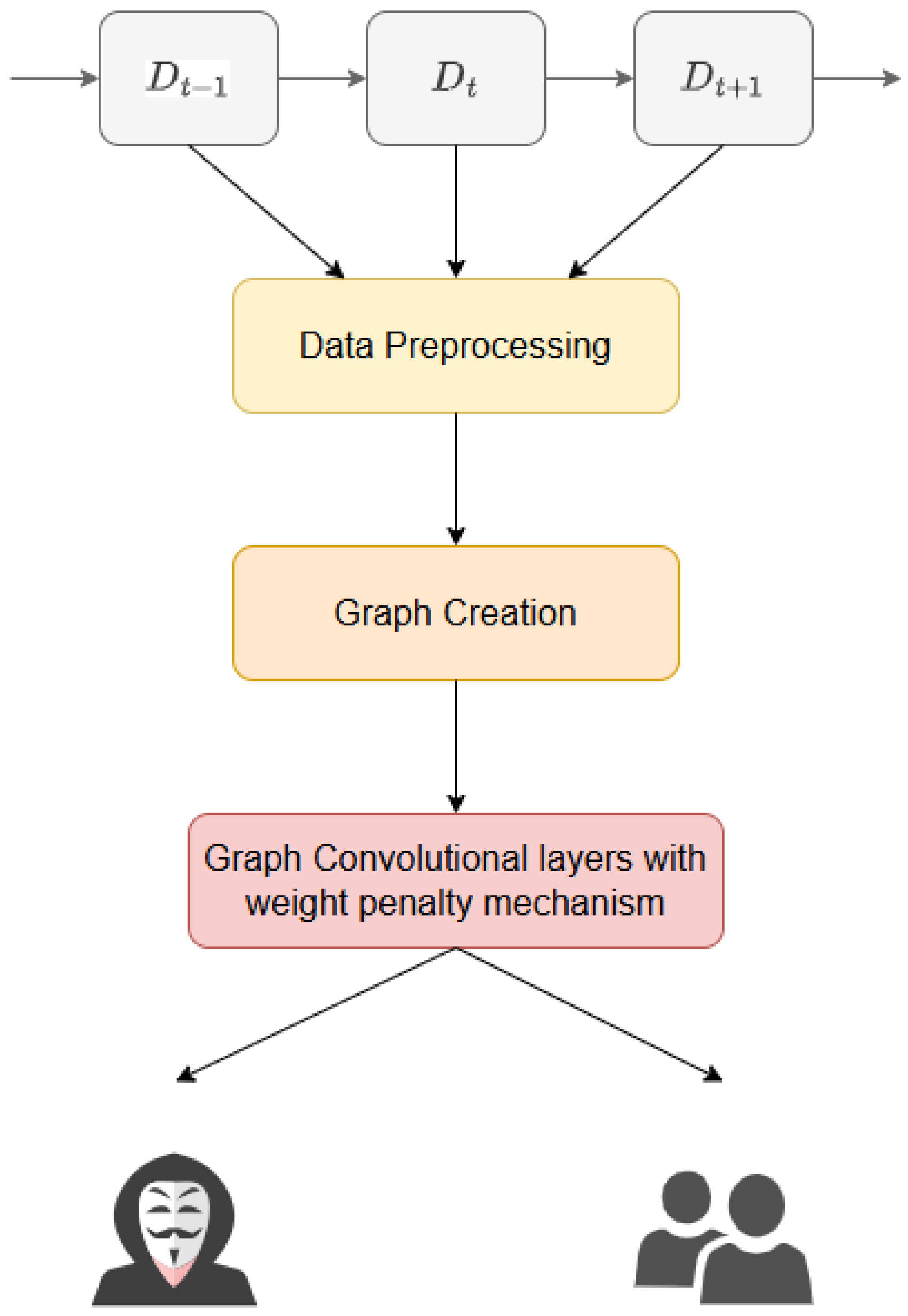
In this work, the proposed model framework is illustrated in Figure 6. Each dataset is treated as a distinct task that is introduced to the model in an incremental manner, reflecting a CL setting. The process begins with data preprocessing, where raw input data undergo necessary transformations to ensure compatibility with subsequent stages. Following this, the data are processed through the graph creation phase in which the dataset is converted into a structured graph representation, enabling effective learning of topological relationships.

Once the graph is constructed, it is fed into the core component of the model, a GCN integrated with a weight penalty mechanism to mitigate CF. This mechanism ensures that important parameters from previously learned tasks are preserved while accommodating new information.

The detailed workflow of the proposed model, including each of these sequential steps, is systematically described in the following subsections.

4.1. Data Preprocessing and Feature Engineering

The authors in [42] have explored the integration of edge features in GNN-based models. Some researchs are successfully implemented an algorithm capable of collecting edge-related information and performing edge classification. However, their approach overlooks crucial endpoint attributes, such as IP addresses and port numbers. This omission is significant as certain network attacks specifically target particular ports. For instance, brute-force attacks commonly focus on ports such as Port 22 and Port 21, which require authentication credentials, making them susceptible to password-cracking attempts. As a result, port information serves as a critical feature for NIDSs, enhancing their ability to detect and classify suspicious network flows effectively. On the other hand, some authors introduced an approach to processing network traffic data by representing SrcIP:SrcPort and DestIP:DestPort as nodes while utilizing other features as edge attributes. This approach systematically constructs unique identifiers through the integration of IP addresses and port information. By consolidating the distinct source and destination port columns into unified fields, it effectively reduces the dimensionality of the dataset, thereby streamlining data representation without compromising essential connection attributes.

Also, there are researches that proposed a method for processing network traffic data by representing Flow IDs as nodes and utilizing other features as edge attributes; they also use random forest for feature selection. This approach aims to generalize the dataset prior to graph construction, allowing for a more structured and scalable representation of network traffic. By defining edges based on selected attributes, this method enhances the ability to capture interactions between different flows. However, a significant limitation of this approach is that it only considers edges between Flow IDs that share the same Source IP. Both of the two approaches have the same limitation, that the constructed graph fails to incorporate critical relationships between flows originating from different sources or targeting different destinations. This omission reduces the overall completeness of the graph structure and may lead to suboptimal performance in intrusion detection tasks, particularly in scenarios where attack patterns involve multiple source and destination pairs. Without a more comprehensive edge definition, the approach risks missing crucial network dependencies, which are essential for accurately identifying complex threats such as DDoS attacks, scanning activities, and coordinated intrusion attempts.

In this study, we propose a novel approach to process network traffic data. We use the LabelEncoder function to encode the string value in the feature column. Additionally, we use the PCC as a simpler and more effective approach to carefully select features. Specifically, in the CIC-IDS-2017 dataset, “TCP Flags count”, which is a new feature, will be the sum of RST Flag Count, SYN Flag Count, URG Flag Count, PSH Flag Count, and ACK Flag Count. The “Flow ID” feature will be changed to the “SourceIP-SourcePort-DestinationIP-DestinationPort” format. After that, we decided to keep the following features: “Flow ID”, “Destination IP”, “Down/Up Ratio”, “Fwd-Bytes”, “Source IP”, “Bwd-Bytes”, “Protocol”, “Total Fwd Packets”, “Total Backward Packets”, “TCP-Flags”, and “Flow Duration”.

The same happens with UNSW-NB15, where the LabelEncoder function is used to encode the string value in the feature column. “Flow ID” feature will be created with the format of “SourceIP-SourcePort-DestinationIP-DestinationPort”.

The complete features of CIC-IDS2017 are listed: Flow ID, Source IP, Destination IP, Protocol, Total Forward Packets, Total Backward Packets, Down/Up Ratio, Fwd_Bytes, Bwd Bytes, TCP Flags, and Flow Duration.

The complete features of UNSW-NB15 are listed: Flow ID, srcip, dstip, proto, sbytes, dbytes, sload, dload, sttl, dttl, and dpkts.

4.2. Graph Creation

For graph creation, as shown in Figure 7, we construct a graph from flow-level data, where each flow is uniquely identified by a tuple of source IP, source port, destination IP, and destination port. In Figure 7, the dataset contains two distinct flows originating from the same source IP (192.168.0.1) to the same destination IP (192.168.0.2) but using different source and destination ports. Each flow entry is represented as a node in the graph, where the node label encapsulates the complete Flow ID (e.g., 192.168.0.1-80-192.168.0.2-5554). Edges between nodes are created based on shared attributes such as common source or destination IPs, representing potential communication or behavior patterns. Since both flows originate from the same source IP, an edge is created between the two nodes, indicating a structural relationship useful for GNNs to learn temporal or behavioral features across related network flows. This structured graph serves as an input to GNNs for tasks like anomaly detection or classification in IDSs.

This methodology ensures a more comprehensive representation of network interactions, effectively capturing the full scope of information available in the dataset, as illustrated in Figure 8. As an attack occurs, the structural relationships within the graph become increasingly dense, reflecting heightened network activity. This increased connectivity enhances the model’s predictive performance by preserving critical information, thereby mitigating the risk of information loss and improving the detection of anomalous network behaviors.

We construct the graph in Figure 8 through the following steps:

• Create a blank graph and then create nodes with the number equal to the number of flow IDs in the dataset. In this case, 16 nodes are created, from node A to node H’.
• Data in all features in dataset are encoded using LabelEncoder function.
• From the “Source IP” feature, if two flow IDs are matching, an edge is created between the two nodes represented by those two flow IDs.
• From the “Destination IP” feature, if two flow IDs are matching, an edge is created between the two nodes represented by those two flow IDs.

4.3. Graph Convolutional Layers with Weight Penalty Mechanism

In the research details illustrated in Figure 9 and Algorithm 1, our proposed model is based on the idea of mixing the representation effectiveness of the GCN model and the weight preservation idea of the regularization-based method in CL. This combination makes the model more resilient to CF and still keeps the high performance of GCN.

Algorithm 1: Training 2-Layer GCN with Elastic Weight Consolidation (EWC)

The model is then subsequently processed by a two-layer GCN to learn embeddings that integrate node features and graph topology. These embeddings are then aggregated into a single graph-level vector representation. This vector serves as input to two consecutive fully connected linear layers for higher-level feature abstraction, followed by a softmax activation function to produce probabilities for the final binary classification. Critically, the model is optimized using a composite loss function that combines the standard binary cross-entropy loss, addressing the current classification task, with a weight penalty regularization term. The component mitigates CF in CL settings by adding a quadratic penalty that discourages changes to parameters identified as important (typically via the Fisher Information Matrix) for tasks learned previously, thus balancing new learning with knowledge retention.

$$L_{\mathrm{task}}=-{\displaystyle \frac{1}{N}}\sum _{i=1}^N\left(y_{i}log\left(P\left(y_i\right)\right)+(1-y_i)log(1-P\left(y_i\right))\right)$$

(8)

where,

$L_{\mathrm{task}}$

: Loss of the current task.

N 

: number of labels.

$y_i$

: the truth value between “Attack” or “Benign”.

$P\left(y_i\right)$

: Softmax probability for the $i_{th}$ task.

$$L_{\mathrm{ewc}}=L_{\mathrm{task}}+\sum _i{\displaystyle \frac{\lambda }{2}}{({\theta }_i-{\theta }_i^A)}^2\mathcal{F}$$

(9)

$$\mathcal{F}=\mathbb{E}\left[-{\displaystyle \frac{{\partial }^{2}log\left(p\left(\theta \right|A)\right)}{{\partial }^2\theta }}{|}_{\theta ={\theta }_A^{*}}\right]$$

(10)

where,

$L_{\mathrm{task}}$

: Loss of the current task.

$\lambda$

: importance of the previous task.

${\theta }_i$

: optimized parameters of the existing task.

${\theta }_i^A$

: optimized parameters of the previous task.

$p\left(\theta \right|A)$

: probability of ${\theta }_i$ after the previous task.

$\mathcal{F}$

: Fisher information matrix.

Formula (9) in our paper represents the loss function adopted for continual learning in our GNN-based IDS framework.

This formulation includes two components:

• The first term, $L_B$, is the binary cross-entropy loss. It measures the prediction error on the current task and helps the model learn the new data.
• The second term is the regularization component from Elastic Weight Consolidation (EWC). It penalizes changes to the parameters ${\theta }_i$ that are important for previous tasks. The Fisher Information Matrix $\mathcal{F}$ quantifies the importance of each parameter, and ${\theta }_i^A$ are the parameter values after training on the previous task.

Compared to the original EWC formulation introduced in our background section, our loss function keeps the core structure but integrates it with a binary classification loss $L_B$, which is more appropriate for the nature of intrusion detection problems. Moreover, in our implementation, the importance weight $\lambda$ is treated as a tunable hyperparameter, chosen based on validation performance. This empirical tuning approach is consistent with many works in the continual learning literature and allows flexibility to adapt the regularization strength depending on the task scenario.

This formulation enables our model to learn new tasks while effectively mitigating catastrophic forgetting, which is critical in practical continual learning settings for cybersecurity.

5. Experiment and Evaluation

This section details the datasets chosen for both training and testing purposes, describes the evaluation metrics utilized to assess experimental performance, and provides an overview of the experimental setup, including the configuration of task-incremental learning scenarios.

5.1. Evaluation Metrics

In this paper, to the best of our knowledge, the results of this study were evaluated using four key performance metrics: accuracy, precision, F-measure, and recall. Each metric yields values ranging from 0 to 1, where values approaching 1 signify superior performance, while those closer to 0 indicate lower effectiveness. The calculation methods for these metrics are detailed in

Table 2. Model performance metrics.

Metric	Definition
Recall	${\displaystyle \frac{TP}{TP+FN}}$
Precision	${\displaystyle \frac{TP}{TP+FP}}$
F1-score	${\displaystyle \frac{2\times \mathrm{Recall}\times \mathrm{Precision}}{\mathrm{Recall}+\mathrm{Precision}}}$
Accuracy	${\displaystyle \frac{TP+TN}{TP+FP+TN+FN}}$

.

where, $TP$ denotes True Positive, $FN$ denotes False Negative, $FP$ denotes False Positive, and $TN$ denotes True Negative.

5.2. Implementation Environment

We implement EL-GNN in two distinct scenarios:

• Implement the EL-GNN on two incremental task and prove the effectiveness of mitigating CF with processing CIC-IDS-2017 as Task A and processing UNSW-NB15 as Task B.
• Implement EL-GNN on a single task and prove the effectiveness single-task prediction quality.

The implementation of the EL-GNN on two incremental tasks is structured using distinct datasets: CIC-IDS-2017 (Task A) and UNSW-NB15 (Task B). Figure 10 shows the process begins with Task A, where raw data from the CIC-IDS-2017 dataset undergo feature selection using a correlation-based technique to retain the most informative features for intrusion detection. The selected dataset is then partitioned into training and testing subsets (Step 2), enabling the development of a GNN-based representation for both the training and test sets (Steps 3a and 3b). The training graph is used to train the initial EL-GNN model (Step 4) to preserve learned parameters critical to Task A (Step 5). The optimized model is then evaluated on the test graph of Task A to assess its classification performance (Steps 6 and 7).

As shown in

Table 3. Comparison of state-of-the-art continual learning models in terms of input, output, architecture, layer size, and activation function.

Model	Input	Output	Architecture	Nodes (One Layer)	Activation Function
SPIDER	Vector (with Task Context)	Class Label	Dynamic Sparse MLP + Replay Buffer	100–512	ReLU, GELU
PAPA	Graph (A, X)	Node Classification	Prototype-based GNN + Pseudo-Replay	128–256	ReLU
ECBRS	Vector (Streaming)	Class Label	Episodic Memory + Encoder–Decoder	64–128	Tanh, ReLU
GEM	Vector	Class Label	Gradient Episodic Memory with Shared MLP	100–256	ReLU

, we observe that most models rely on vectorized input representations, with the exception of PAPA, which directly utilizes graph-structured data—a notable distinction in the context of GNN-based applications. In terms of output, all models perform classification tasks, although PAPA is specifically tailored for node classification within graphs. Architecturally, the models vary significantly: SPIDER employs dynamic sparse MLPs with replay buffers, while PAPA leverages prototype-based GNNs coupled with pseudo-replay mechanisms. ECBRS introduces an encoder–decoder structure with episodic memory, and GEM utilizes gradient-based memory updates in shared MLP frameworks. The layer sizes also differ widely, ranging from compact 64-node configurations to more expansive 512-node layers, reflecting trade-offs between model complexity and scalability. Activation functions further highlight diversity in design, with ReLU being the most common choice, sometimes combined with GELU or Tanh for specific optimization behaviors. Overall, this comparison underscores the varying approaches and assumptions made in existing continual learning frameworks, many of which differ from our GNN-based IDS context both in data structure and task formulation.

After testing Task A, Figure 10 also shows that Task B leverages the UNSW-NB15 dataset, where features are similarly selected using correlation analysis before the dataset is split into training and test sets (Step 9). Graph representations are constructed from these subsets (Steps 10a and 10b), and the EL-GNN model, initially trained on Task A, is further trained on the training graph of Task B (Step 11). During this phase, CL is enforced through EWC (Step 12), enabling the model to adapt to new data while mitigating CF of previously acquired knowledge. After this optimization, the model is tested not only on the test graph of Task B (Step 13) but also reevaluated on the test graph of Task A (Step 14) to quantify knowledge retention. Finally, classification results are produced based on the optimized model’s performance across both tasks (Step 15).

The implementation of the EL-GNN on a single existing task, detailing the internal steps before it is incorporated into a CL setup. Figure 11 shows the process begins with the input of an existing intrusion detection dataset (Step 1), which is subjected to a feature selection process based on a correlation analysis technique (Step 2). The selected features are then split into training and test datasets (Steps 2a and 2b), preparing the data for graph construction. These subsets are each transformed into GNN-based representations—the training dataset into a training graph (Step 3a) and the test dataset into a test graph (Step 3b)—enabling the model to exploit structural relationships among data points. The training graph is used to train the EL-GNN model (Step 4), which captures the underlying patterns in the data. Following this, the model is optimized (Step 7) to enhance generalization and mitigate overfitting or forgetting in subsequent tasks. The optimized model is then evaluated on the test graph (Step 6), and its performance is used to produce the final classification outcomes (Step 8). This workflow serves as the foundational unit in a CL pipeline, allowing for modular training and evaluation of the EL-GNN on individual tasks prior to sequential integration across multiple datasets.

We conducted the experiment in the following environment:

• GPU: TESLA K80.
• CPU: Intel(R) Core i7-8700.
• RAM: 48 GB.

For the model’s parameter, the learning rate, which determines the step size in the gradient descent process, plays a critical role in influencing the model’s ability to converge to a global optimum. To identify suitable parameter values, a series of controlled experiments were conducted wherein individual parameters were varied, while others were held constant. The experimental results demonstrated that the model attained its optimal performance under the configuration where the number of hidden units was set to 500 and the learning rate was maintained at 0.001. The training procedure was conducted over a total of 3000 epochs, during which the model parameters were optimized using the Adam optimization algorithm. Throughout the training process, the cross-entropy loss function was employed as the objective metric to guide the minimization of classification errors. This combination of hyperparameter settings and optimization strategy contributed significantly to the model’s ability to effectively learn from the data and achieve high accuracy.

5.3. Evaluation

In our work, the datasets we selected CIC-IDS2017 and UNSW-NB15 are among the most widely recognized and widely used in the intrusion detection research community. These datasets represent diverse types of attacks, network environments, and traffic characteristics. By using them as two distinct tasks, we ensure our approach is evaluated under practical and high-impact scenarios. In future work, we plan to incorporate more datasets or real-world streaming data to extend our experimental setup and further explore the robustness of our method in larger-scale continual learning scenarios.

Our analysis emphasized the stability of the model, as evidenced by its convergence behavior. This stability is illustrated by the training progress shown in Figure 10 and Figure 11. Utilizing the previously specified parameters, the proposed model approaches convergence near the 600th epoch and maintains consistent performance thereafter.

Subsequently, the accuracy attained by the model during the testing phase highlights its capability to reliably detect malicious flows within network environments. This high level of detection effectiveness indicates that the proposed model possesses sufficient robustness for practical deployment in organizational and enterprise network systems. For evaluation, twenty percent of each dataset was allocated for testing, comprising 84,831 flows from the CIC-IDS2017 dataset and 9997 flows from the UNSW-NB15 dataset, respectively.

The model’s prediction outcomes are illustrated in the confusion matrices shown in Figure 12 and Figure 13. Analysis of these results reveals that the total proportion of incorrect predictions—including both false positives and false negatives—is below 1%. This low error rate demonstrates that the model consistently attains a high detection accuracy for both malicious and benign network flows.

Figure 14 and Figure 15 depict the model’s performance in detecting malicious flows across two test datasets through Receiver Operating Characteristic (ROC) curves. Given the class imbalance present within the datasets, the evaluation prioritized the weighted F1-score rather than relying exclusively on accuracy. The weighted F1-score was calculated by aggregating the F1 scores of individual flow categories, each weighted according to their respective representation within the test dataset, thereby providing a more balanced and informative assessment of the model’s detection capabilities.

As illustrated in Figure 16 and Figure 17, our proposed model achieves remarkable accuracy levels of 99.76% and 98.65% on the CIC-IDS2017 and UNSW-NB15 datasets, respectively.

These high accuracy rates indicate that the model consistently performs well in correctly identifying both malicious and benign network flows. Such consistent detection capability underscores the model’s robustness, reliability, and overall effectiveness across a variety of intrusion detection scenarios and network environments.

5.4. Comparison with Other Graph Models

To thoroughly evaluate the effectiveness of the proposed model, we conducted an extensive comparative analysis by measuring its testing accuracy against several leading GNN-based models that are currently recognized as highly effective within the domain of intrusion detection. Our evaluation specifically focused on benchmarking against well-established models, including E-GraphSAGE, E-ResGAT, and conventional GCNs, all of which have demonstrated strong performance in related tasks. For this comparative study, we carefully implemented the E-GraphSAGE and GCN models according to the architectures and methodologies presented in their original research papers. We then applied these models to the task of classifying malicious network flows using two widely adopted benchmark datasets: CIC-IDS2017 and UNSW-NB15. It is important to note that the E-GraphSAGE model distinguishes itself by extracting edge features directly from network flow data and leveraging these features for edge-level classification tasks. In contrast, the traditional GCN model utilizes flow data as node features, embedding the information within the nodes themselves rather than the edges. This fundamental difference in how flow data are incorporated into the graph structure provides a meaningful basis for comparing the strengths and limitations of each approach and helps highlight the unique contributions of our proposed model within this context.

The effectiveness of the proposed EL-GNN model was rigorously evaluated using two benchmark intrusion detection datasets: CIC-IDS-2017 and UNSW-NB15, under both static and CL scenarios. As shown in Figure 18 and Figure 19 in the absence of CF, the EL-GNN achieves competitive test accuracies of 96.72% and 98.44% on CIC-IDS-2017 and UNSW-NB15, respectively. While these results are slightly lower than those of state-of-the-art models such as the FN-GNN, which report accuracies above 96% while training with the CIC-IDS-2017 dataset and 96.9% while training with the UNSW-NB15 dataset, this still confirms that the EL-GNN performs comparably in conventional settings and establishes a strong baseline for more dynamic learning conditions.

As in the scope of this research, our proposed method is not necessarily to surpass the performance of single-task models. In continual learning, especially under a task-incremental scenario, the key challenge is to mitigate catastrophic forgetting—the tendency of a model to lose performance on old tasks when trained on new ones. As a result, our model may not outperform state-of-the-art single-task models, which are trained with full access to task-specific data and are optimized solely for one task without needing to retain prior knowledge.

Importantly, during continual training, we do not revisit old data. As a result, the model naturally biases toward the new task due to the dominance of the new data in the optimization process. To counteract this bias and rebalance the learning process, we introduce the hyperparameter $\lambda$ in the EWC term. This parameter increases the influence of the previous task’s knowledge and prevents it from being overwritten.

The true strength of the EL-GNN becomes evident in CL scenarios, shown in Figure 20, where CF significantly hampers the performance of conventional GNN models. When sequential learning is introduced, other models experience substantial drops in accuracy: for example, the FN-GNN drops from 94.9% to 49.9% and E-GraphSAGE from 95.2% to 55.2%. This reflects a remarkable resilience to forgetting, attributed to the integration of regularization-based methods, which effectively preserve crucial model parameters learned from prior tasks.

These results, especially

Table 4. Comparison of model test Accuracy (%) with different scenarios.

Model	CIC-IDS-2017	UNSW-NB15	Incremental Task
FN-GNN	96.90%	98.52%	49.9%
E-GraphSAGE	95.67%	97.54%	55.2%
GCN	96.53%	96.45%	63.9%
E-ResGAT	94.92%	97.92%	44.6%
EL-GNN	96.72%	98.44%	85.7%

, demonstrate that while the EL-GNN may not always lead in static accuracy benchmarks, it significantly outperforms existing models in dynamic environments where CL is necessary. Therefore, the EL-GNN is particularly well suited for real-world network security applications, where models must adapt to evolving threats without compromising previously acquired knowledge. Its consistent performance across datasets highlights its potential as a reliable and scalable solution for GNN-based intrusion detection in ever-changing cybersecurity.

When we evaluate the model using the F1-score for an imbalanced dataset, we come up with the results in Figure 21 and Figure 22.

As shown in Figure 21, Figure 22 and

Table 5. Comparison of model F1-score with different scenarios.

Model	CIC-IDS-2017	UNSW-NB15
FN-GNN	0.9572	0.9728
E-GraphSAGE	0.9447	0.9374
GCN	0.9156	0.9567
E-ResGAT	0.9245	0.9654
EL-GNN	0.9572	0.9697

, across both datasets, the proposed EL-GNN model consistently achieves the highest F1-scores: 0.9682 and 0.9728 on CIC-IDS-2017 and UNSW-NB15, respectively. This demonstrates model’s strong generalization ability and robust performance across different network intrusion scenarios. Notably, the EL-GNN outperforms competitive baselines such as the FN-GNN and E-ResGAT, which are known for their feature refinement and residual structures, respectively. While models like the GCN and E-GraphSAGE perform reasonably well, their lower F1-scores indicate less effectiveness in capturing complex attack patterns. These results highlight EL-GNN’s capability to extract discriminative representations while preserving performance across datasets, validating its suitability for real-world intrusion detection tasks.

5.5. Comparison with Other CL Models

As there is no formula for Lambda, because each dataset has different lambda settings suitable for that dataset, we have implemented the model in incremental task scenarios with a range of lambda from 50 to 200 with a step of 25. The result is shown in the Figure 23.

As shown in Figure 23, after carefully choosing Lambda 100 and 150 as the two most effective parameters, we proposed the hyperparameters as seen in

Table 6. Hyperparameter comparison between SPIDER, PAPA, ECBRS, GEM, and EL-GNN.

Model	Learning Rate	Batch Size	Optimizer	Memory Size	Regularization
SPIDER	0.0005	128	AdamW	500 samples	Weight Decay = ${10}^{-4}$
PAPA	0.001	64	Adam	200 pseudo-prototypes	Dropout = 0.3
ECBRS	0.01	32	SGD + Momentum	Episodic buffer = 100	Weight Decay = $5\times {10}^{-4}$
GEM	0.001	64	Adam	Episodic memory = 256	Dropout = 0.2
EL-GNN	0.001	32 (with CIC-IDS-2017)	Adam	Not required	Dropout = 0.5, EWC $\lambda =100$
EL-GNN	0.001	64 (with UNSW-NB15)	Adam	Not required	Dropout = 0.5, EWC $\lambda =150$

.

Our work focuses on tackling continual learning challenges in the context of GNN-based IDSs, a relatively underexplored area. To the best of our knowledge, there are currently no existing methods that directly address continual learning for GNNs in IDS settings. As a result, we selected representative and widely accepted continual learning baselines—such as PAPA, SPIDER, EWC, MAS, and ECBRS—which, while originally designed for generic neural networks, serve as foundational methods for evaluating catastrophic forgetting and knowledge retention. Additionally, we included comparisons with existing GNN-based IDS models and continual learning approaches in the IDS literature, which are the most relevant available works to date. These choices aim to position our work within both the GNN-based IDS and continual learning research communities.

The proposed EL-GNN model demonstrates notable effectiveness in addressing the challenges of CL for IDSs, significantly outperforming several state-of-the-art methods. As shown, Figure 24, Figure 25 and

Table 7. Comparison of our model to state-of-the-art model with different evaluation metrics.

Model	F1-Score	Accuracy
PAPA	0.9347	85.7%
SPIDER	0.9235	83%
ECBRS	0.9356	82.3%
EWC	0.8945	84.2%
MAS	0.8467	82.1%
EL-GNN	0.9578	84.5%

further validate the robustness and generalization of the proposed model. The EL-GNN achieves 85.7% accuracy, again outperforming PAPA (83.0%), SPIDER (82.3%), ECBRS (84.2%), EWC (82.1%), and MAS (84.5%). This consistent superiority across datasets highlights the model’s ability to maintain high detection performance across varying network environments and attack patterns. Notably, the scenarios where the CIC-IDS-2017 and UNSW-NB15 datasets form two incremental tasks present a more complex and realistic traffic scenario, indicating that the EL-GNN is well suited for real-world deployments where CL and adaptation are essential. In contrast, traditional methods like EWC either suffer from reduced performance due to insufficient retention of previously learned knowledge or limited flexibility in learning new patterns. The EL-GNN, on the other hand, strikes a balance between stability and plasticity through its elastic consolidation mechanism, enabling it to preserve critical knowledge while maintaining adaptability in evolving cyber threat landscapes.

The experimental results clearly indicate that the EL-GNN achieves the best overall performance among the compared CL methods. Its consistent accuracy gains across both datasets demonstrate its effectiveness in overcoming the limitations of CF while sustaining high detection rates. The synergy between elastic weight consolidation and GNN-based representation learning proves to be a powerful paradigm for CL in the context of network intrusion detection. This makes the EL-GNN a compelling and practical solution for deployment in modern, dynamic cybersecurity infrastructures where ongoing learning from streaming data is crucial.

6. Conclusions

In this study, we proposed the EL-GNN model, a comprehensive framework encompassing feature and data preprocessing, graph construction, and a novel Graph Convolutional Network (GCN) architecture integrated with a weight penalty mechanism. We introduced an innovative method to represent network flow data as graph structures, where nodes correspond to unique Flow IDs and edges are established based on shared source and destination IP addresses. The selection of these edges is guided by correlation-based algorithms to accurately capture the relationships between flows, effectively modeling network communication patterns. Our modified GCN architecture incorporates a weight penalty mechanism that synergistically combines traditional GCN techniques with regularization-based continual learning strategies. This integration effectively mitigates the problem of catastrophic forgetting (CF) commonly encountered in prior GNN-based models, thereby enhancing the model’s stability and generalization capabilities.

The proposed EL-GNN demonstrated high stability during training and achieved impressive accuracy scores of 95.9% and 96.4% on the CIC-IDS2017 and UNSW-NB15 benchmark datasets, respectively. Furthermore, in incremental-task training scenarios, the model attained a promising accuracy of 85.7%, highlighting its effectiveness in continual learning contexts. The experimental results confirmed the robustness of the EL-GNN in accurately classifying both normal and malicious network flows, surpassing the performance of recent state-of-the-art approaches in the domain.

Despite these achievements, we acknowledge that the dynamic and ever-evolving nature of network threats necessitates continual adaptation and improvement of intrusion detection systems. To address this, future work will focus on updating and fine-tuning the EL-GNN model with emerging datasets and evolving threat patterns, ensuring sustained effectiveness in detecting increasingly complex and sophisticated attack scenarios in real-world deployments.