Partial Ambiguity Resolution Strategy for Single-Frequency GNSS RTK/INS Tightly Coupled Integration in Urban Environments

Abstract

Single-frequency global navigation satellite system/inertial navigation system (GNSS/INS) integration has wide application prospects in urban environments; however, correct integer ambiguity is the major challenge because of GNSS-blocked environments. In this paper, a sequential strategy of partial ambiguity resolution (PAR) of GNSS/INS for tightly coupled integration based on the robust posteriori residual, elevation angle, and azimuth in the body frame using INS aids is presented. First, the satellite is eliminated if the maximum absolute value of the robust posteriori residuals exceeds the set threshold. Otherwise, the satellites with a minimum elevation angle of less than or equal to 35° are successively eliminated. If satellites have elevation angles greater than 35°, these satellites are divided into different quadrants based on their azimuths calculated in body frame. The satellite with the maximum azimuth in each quadrant is selected as the candidate satellite, the candidate satellites are eliminated one by one, and the remaining satellites are used to calculate the position dilution of the precision (PDOP). Finally, the candidate satellite with the lowest PDOP is eliminated. Two sets of vehicle-borne data with a low-cost GNSS/INS integrated system are used to analyze the performance of the proposed algorithm. These experiments demonstrate that the proposed algorithm has the highest ambiguity fixing rates among all the designed PAR methods, and the fixing rates for these two sets of data are 99.40% and 98.74%, respectively. Additionally, among all the methods compared in this paper, the proposed algorithm demonstrates the best positioning performance in GNSS-blocked environments.

1. Introduction

The integrated navigation of multi-system global navigation satellite system/inertial navigation system (GNSS/INS) has wide application prospects in intelligent driving, intelligent transportation, and vehicle navigation [1]. The real-time kinematic (RTK) method is an effective technique for obtaining centimeter-level positioning in kinematic environments, and the integration of GNSS RTK and INS has been widely researched. The fast, reliable, and correct confirmation of the integer ambiguity is key for the high-accuracy positioning of GNSS RTK/INS integration navigation. However, in GNSS-blocked environments, such as urban canyons, viaducts, and tree-lined roads, multipath (MP) effects and non-line-of-sight (NLOS) conditions interfere with GNSS observations [2,3,4]. The ambiguity fixing performance is affected by low-quality observations [5]. Therefore, it is important to develop a method to deal with low-quality observations to obtain reliable and correct integer ambiguities in complex urban environments.

In GNSS-blocked environments, there may be more contaminated observations, and it is difficult and unnecessary to fix the full ambiguities [6]. The partial ambiguity resolution (PAR) strategy has been proposed, which aims to resolve a corrected subset of ambiguities instead of the full ambiguity resolution (FAR) [7,8,9]. Generally, the methods of the ambiguity subset selection for single-frequency users can be divided into two categories: methods based on observation characteristics and methods based on the metric indication of ambiguity quality [6]. The common subset selection method based on observation characteristics uses the elevation angle and signal-to-noise ratio (SNR) [10,11,12]. However, the observation may be contaminated by NLOS and MP effects when the satellite has a high elevation angle and SNR in GNSS-blocked urban environments [13]. Variance is an important metric for expressing the accuracy of estimated parameters [14,15,16], and the ambiguity dilution of precision (ADOP) reflects an intrinsic measure for the average precision of the ambiguities [17,18]. These metric indications can be used to determine the ambiguity subset. However, these methods ignore the ambiguity biases that are contaminated by GNSS-blocked environments, which degrades the performance of PAR based on these metric indications [9].

To improve the performance of ambiguity fixing, the method of combining different strategies has been researched. Parkins proposed a PAR method based on the ADOP and average SNR [11]. The elevation angle and ADOP have been combined to select the ambiguity subset [19]. To reduce the MP impact, the PAR method based on elevation and the SNR was proposed for high-accuracy positioning in canyon environments [12]. To improve the AR performance, Li et al. [15] combined the elevation angle and decorrelation variances to select the ambiguity subset. In kinematic urban areas, the GNSS observations are susceptible to MP and NLOS interference, and the performance of the ambiguity fixing of the above methods may deteriorate [20]. Usually, the residual can reflect the observation quality, and the method of ambiguity subset selection combined with the residual has been researched. The abnormal observations will lead to estimated parameter bias, and the effect of abnormal observation can be decreased using the robust estimation method [21]. Li et al. [6] proposed a sequential ambiguity selection strategy based on the posterior residual, elevation angle, and decorrelation variance to handle abnormal observation, and the quality control algorithm based on robust estimation was used to reduce the impact of gross errors. To improve the position reliability of the SF GNSS in urban environments, Chai et al. [22] proposed a PAR method based on the robust posteriori residual and elevation angle, and the fixing rate of the ambiguity was improved. However, it is challenging to correctly detect abnormal observations when there are multiple gross errors [2,23]. The environmental feature can be used to select high-quality satellites. The 3D map can be used to classify line-of-sight and NLOS signals. However, this method needs the previously known 3D city model [24]. Yin et al. [25] proposed an algorithm for satellite selection based on sky-pointing images to detect the sky and non-sky areas, and these satellites in the sky area are selected for positioning. An additional visual sensor is needed for the method of satellite selection.

In urban areas, environmental features of a large number of narrow and long scenes exist, such as roads bordered by tall buildings and dense trees. In such scenes, the forward and backward directions of the roads are open, and the two sides are seriously blocked environments. The satellites located in the forward and backward directions of roads may have a higher quality than those located on the two sides of the roads. The azimuth of the satellite in the body plane frame can be used to locate where it is. Therefore, the environmental feature is researched to select high-quality satellites in this research. There are continuous and complex GNSS-blocked environments in urban areas, and the single strategy used to select the ambiguity subset is unreliable, especially for an SF GNSS. A sequence algorithm for PAR based on the robust posteriori residual, elevation angle, azimuth, and position dilution of precision (PDOP) for SF GNSS RTK/INS tightly coupled (TC) integration is developed in this study. The TC integration model of the SF GNSS RTK/INS and the sequence strategy for PAR are discussed in Section 2. In Section 3, the performance of the proposed algorithm using vehicle-borne data is analyzed. Section 4 presents the conclusions.

2. Materials and Methods

2.1. Tightly Coupled Integration of SF GNSS RTK/INS

2.1.1. System Model of Tightly Coupled Integration

The extended Kalman filter (EKF) is used to solve the TC integration of the SF GNSS RTK/INS. The system model of SF GNSS/INS TC integration is obtained using the INS error model, and the phi-angle error model of the local navigation frame can be expressed as follows [26]:

$$\begin{array}{l}\stackrel{•}{{\varphi }^n}=-\left({\omega }_{ie}^n+{\omega }_{en}^n\right)\times {\varphi }^n+\delta {\omega }_{in}^n-C_b^n\delta {\omega }_{ib}^b\\ \delta \stackrel{•}{v^n}=f^n\times {\varphi }^n-\left(2{\omega }_{ie}^n+{\omega }_{en}^n\right)\times \delta v^n-\left(2\delta {\omega }_{ie}^n+\delta {\omega }_{en}^n\right)\times v^n+C_b^n\delta f^b+\delta g^n\\ \delta \stackrel{•}{r^n}=-{\omega }_{en}^n\times \delta r^n+\delta v^n\end{array}$$

(1)

where the superscripts $n$ and $b$ are the local navigation frame ($n$-frame) and the body frame ($b$-frame); the subscripts $i$ and $e$ denote the inertial frame ($i$-frame) and the earth-centered and earth-fixed frame ($e$-frame); and ${\varphi }^n$, $\delta v^n$, and $\delta r^n$ are the attitude, velocity, and position error vectors, respectively. Additionally, ${\omega }_{ie}^n$ is the Earth’s rotation velocity, and ${\omega }_{en}^n$ is the angular velocity of the $e$-frame with respect to the $i$-frame; $f^n$ is the specific force in the $n$-frame; and $C_b^n$ is the direction cosine matrix (DCM) from the $b$-frame to the $n$-frame. Furthermore, $\delta f^b$ and $\delta {\omega }_{ib}^b$ are the accelerometer and gyroscope output errors in the $b$-frame, respectively; $\delta g^n$ is the gravity error vector.

In this research, the state vectors include the misalignment angle, velocity error, position error, accelerometer bias error, and gyroscope bias error. The error state equation can be expressed as follows:

$${\stackrel{•}{X}}_k=F_k{X}_k+G_k{w}_k$$

(2)

where $X_k=\left[\begin{array}{ccccc}{\varphi }^n& \delta v^n& \delta r^n& \delta b_a& \delta b_g\end{array}\right]$, and $\delta b_a$ and $\delta b_g$ are the accelerometer bias error and gyroscope bias error; ${\omega }_k$ is the system noise vector; and $F_k$ and $G_k$ are the coefficient matrices of the error state vectors and drive matrix of the noise.

2.1.2. Observation Model of Tightly Coupled Integration

In this paper, the pseudo-range and carrier phase observations of the first frequency are used for double-difference (DD) SF GNSS positioning. The global positioning system (GPS), BeiDou Navigation Satellite System (BDS), and Galileo satellites are used for difference positioning, and the individual GNSS is applied to construct the DD observation equation [27]. The highest elevation angle of each satellite system is used as the reference satellite. The ionospheric delay and tropospheric delay can be ignored after the double difference for a short baseline, and the DD observation equations of the pseudo-range and carrier phase are simplified as follows:

$$\Delta \nabla P_{mn}^{\ast ,sr}=\Delta \nabla {\rho }_{mn}^{\ast ,sr}+\Delta \nabla {\epsilon }_{mn,P}^{\ast ,sr}$$

(3)

$$\lambda \Delta \nabla {\phi }_{mn}^{\ast ,sr}=\Delta \nabla {\rho }_{mn}^{\ast ,sr}+\lambda \Delta \nabla N_{mn}^{\ast ,sr}+\Delta \nabla {\epsilon }_{mn,\phi }^{\ast ,sr}$$

(4)

where $\Delta \nabla$ is the DD operator; the superscript * denotes different satellite systems; the superscripts $s$ and $r$ denote the satellite numbers; and the subscripts $m$ and $n$ represent the observation stations. Additionally, $P$ and $\phi$ are the pseudo-range and carrier phase observations, respectively; $\rho$ is the geometric distance between the satellite and receiver; $N$ is the ambiguity; $\lambda$ is the wavelength; and ${\epsilon }_{mn,P}^{sr}$ and ${\epsilon }_{mn,\phi }^{sr}$ are the noise of the pseudo-range and carrier phase observations, respectively.

In this research, the decentralized model is used for the TC integration of the GNSS RTK/INS. First, the ambiguities are resolved by linearizing Equations (3) and (4),

$$\left[\begin{array}{c}\Delta \nabla P-\Delta \nabla {\rho }_{INS}\\ \Delta \nabla \phi -\Delta \nabla {\rho }_{INS}\end{array}\right]=\left[\begin{array}{cc}{H}_k& 0_k\\ H_k& I_k\end{array}\right]\left[\begin{array}{c}{X}_k\\ \nabla \Delta N_k\end{array}\right]+\left[\begin{array}{c}\Delta \nabla {\epsilon }_P\\ \Delta \nabla {\epsilon }_{\phi }\end{array}\right]$$

(5)

where $H_k$ is the coefficient matrix of the observation equation; $I_k$ is the unit matrix. ${\rho }_{INS}=‖r_{INS}^e-r_s^e‖$, where $‖•‖$ is the modulo operation, $r_s^e$ is the satellite coordinates, and $r_{INS}^e$ is the receiver coordinates calculated by the INS.

Equation (5) is used to solve the float ambiguities and their variance–covariance matrix. The least-squares ambiguity decorrelation adjustment (LAMBDA) method is used to search the integer ambiguities. The ratio value, the success rate of ambiguity fixing, and the unit weight of the standard error are used to confirm the integer ambiguities [22]. When these ambiguities are fixed, the integer ambiguities can be used as the high-accuracy observation, and the observation model of the SF GNSS RTK/INS tightly coupled integration is as follows:

$$Z_k=\left[\Delta \nabla \phi -\Delta \nabla {\rho }_{INS}-\lambda \Delta \nabla \stackrel{⌣}{N}\right]=H_k{X}_k+{\eta }_k$$

(6)

where $Z_k$ is the observation vector; $\Delta \nabla \stackrel{⌣}{N}$ is the integer ambiguity; and ${\eta }_k$ is the observation noise. The EKF is used to solve Equation (6) for the parameter estimation, and the robust estimation algorithm based on the Institute of Geodesy and Geophysics III (IGG-III) algorithm is used to reduce the impact of observation errors.

$$X_k={\Gamma }_k^{-}{H}_k^T{\left(H_k{\Gamma }_k^{-}{H}_k^T+\gamma R_k\right)}^{-1}\left(Z_k-H_k{X}_{k-1}\right)$$

(7)

where ${\Gamma }_k^{-}$ is the predicted variance matrix; $R_k$ is the matrix of observation noise; and $\gamma$ is the weight factor, which can be obtained as follows [28]:

$${\gamma }_i=\left\{\begin{array}{cc}1& \left|{\overline{v}}_i\right|<k_0\\ {\displaystyle \frac{k_0}{\left|{\overline{v}}_i\right|}}•{\displaystyle \frac{{\left(k_1-\left|{\overline{v}}_i\right|\right)}^2}{{\left(k_1-k_0\right)}^2}}& k_0\le \left|{\overline{v}}_i\right|<k_1\\ 0& k_1\le \left|{\overline{v}}_i\right|\end{array}\right.$$

(8)

where ${\overline{v}}_i$ is the normalized residual; $k_0$ is the quantile parameter; and $k_1$ is the elimination point.

If the full ambiguities cannot be fixed, the sequence strategy of the PAR strategy is performed. The proposed PAR algorithm is described in Section 2.2.

2.2. The Sequence Strategy of the PAR for the SF GNSS RTK/INS Tightly Coupled Integration

The reliable and correct integer ambiguities are key to calculating the high-accuracy position. In urban environments, GNSS signals are susceptible to interference, which affects the fixing performance of ambiguity. In this section, a strategy based on the robust posteriori residual, elevation angle, and azimuth in the body plane frame for PAR is proposed.

2.2.1. The Ambiguity Subset Selection Based on the Robust Posteriori Residual

The filtered residual can reflect the quality of the observation, and the DD carrier phase residuals can be used to measure the quality of the ambiguity estimates. The gross error of an individual observation affects the other observations, and the robust estimation based on the IGG-III algorithm is used to calculate the posteriori residual. The scheme of ambiguity subset selection based on the robust posteriori residual is as follows.

If these integer ambiguities do not pass confirmation, the optimal solution of the integer ambiguities $\Delta \nabla \widehat{N}$ that is searched using the LAMBDA method is substituted into Equation (4) to calculate the residuals of the DD carrier phase observations.

$$V=HX-L$$

(9)

where $L=\left[\lambda \Delta \nabla \phi -\Delta \nabla {\rho }_{INS}+\lambda \Delta \nabla \widehat{N}\right]$; $V$ is the residual.

The least-squares (LS) method is used to calculate Equation (9). However, the LS method has the characteristic of equalization error, and the single gross error of the observation will cause the estimated parameters to crash, thus affecting the residual result of the other observations [22]. Therefore, the robust estimation algorithm is used to adjust the weight of the normalized filtered residual.

$$\widehat{X}={\left(H^T\widehat{\Sigma }H\right)}^{-1}\left(H^T\widehat{\Sigma }L\right)$$

(10)

where $\widehat{X}$ is the posteriori position parameter; $\widehat{\Sigma }=\gamma \sum$ is the equivalent weight; and $\Sigma$ is the weight matrix of observations, which can be calculated using the stochastic model based on the elevation angle. Based on the law of error propagation, the weight value of the DD observation model can be expressed as follows [3]:

$${\Sigma }^{-1}=\left[\begin{array}{cccc}{q}_1^2& p_{1,2}^2& \dots & p_{1,k-1}^2\\ p_{1,2}^2& q_2^2& \dots & p_{2,k-1}^2\\ ⋮& ⋮& \ddots & ⋮\\ p_{1,k-1}^2& p_{2,k-1}^2& \dots & q_{k-1}^2\end{array}\right]$$

(11)

where $q^2={\left({\sigma }_m^s\right)}^2+{\left({\sigma }_m^r\right)}^2+{\left({\sigma }_n^s\right)}^2+{\left({\sigma }_n^r\right)}^2$, $p^2={\left({\sigma }_m^r\right)}^2+{\left({\sigma }_n^r\right)}^2$, and $\sigma ={\displaystyle \frac{{\sigma }_{\sum }}{\sin \theta }}$; $\theta$ is the elevation angle and ${\sigma }_{\sum }$ is the accuracy of observation.

The robust posteriori residual ${\widehat{v}}_i$ can be obtained via the robust iteration estimation of Equation (10). These satellites are sorted based on the absolute values of ${\widehat{v}}_i$, and these satellites are eliminated one by one when the maximum absolute value exceeds the set threshold. If the remaining ambiguities cannot be fixed, the subset selection of ambiguities is based on the elevation angle and azimuth in the body plane frame.

2.2.2. The Ambiguity Subset Selection Based on the Elevation Angle and Azimuth in the Body Plane Frame

In some environments, the higher the elevation angle, the better the quality of the observation, and the elevation angle is used for ambiguity selection. In this paper, 35° is selected as the boundary to distinguish between high and low elevation angles [29]. The satellites are sorted according to their elevation angles, and satellites with elevation angles of less than or equal to 35° are successively eliminated. Otherwise, the ambiguity subset is selected based on the satellite azimuth in the body plane frame.

In urban areas, narrow and long scenes exist. There are obstructions on both sides of the road, and the areas in front of and behind the road are open (Figure 1). Therefore, in this paper, we propose a satellite selection method based on the azimuth in the body plane frame, and the PDOP is used to avoid poor geometry.

The high-accuracy position predicted by the INS is converted to the center of the GNSS antenna, and the converted position is used as the vehicle’s position. The distance vector from the satellite to the GNSS antenna can be obtained as follows:

$${\rho }_{i,s}^e=\left(\nabla X_{i,s}^e,\nabla Y_{i,s}^e,\nabla Z_{i,s}^e\right)=\left(X_s^e,Y_s^e,Z_s^e\right)-\left(X_i^e,Y_i^e,Z_i^e\right)$$

(12)

where $\left(X_s^e,Y_s^e,Z_s^e\right)$ is the position of the satellite in the $e$-frame, and $\left(X_i^e,Y_i^e,Z_i^e\right)$ is the position of the GNSS antenna calculated using the INS. The distance vector ${\rho }_{i,s}^e$ in the $e$-frame is transformed to the $b$-frame using the DCM:

$${\rho }_{i,s}^b=\left(\nabla X_{i,s}^b,\nabla Y_{i,s}^b,\nabla Z_{i,s}^b\right)={\left(C_b^n\right)}^T{C}_e^n{\rho }_{i,s}^e$$

(13)

The plane on which the X- and Y-axes of the $b$-frame are located is defined as the body plane frame, and the body plane frame is divided into four quadrants in the clockwise direction (Figure 2). The satellites can be divided into different quadrants according to the signs of $\nabla X_{i,s}^b$ and $\nabla Y_{i,s}^b$.

The satellite azimuth in the body plane frame can be calculated as follows:

$$\gamma =\arctan \left(\left|{\displaystyle \raisebox{1ex}{$\nabla X_{i,s}^b$}\!\left/ \!\raisebox{-1ex}{$\nabla Y_{i,s}^b$}\right.}\right|\right)$$

(14)

where $\gamma$ is the satellite azimuth in the body plane frame, and $\arctan \left(•\right)$ is the arctan function.

The azimuth range of quadrants I–IV is converted into the range of 0–90°. The satellites in each quadrant are sorted based on azimuth $\gamma$, and the satellite in each quadrant with the maximum azimuth is selected as the candidate satellite to be eliminated. The candidate satellites are eliminated one by one, and the remaining satellites are used to calculate the PDOP. The satellites that participate in the positioning resolution should have a suitable geometry, and the candidate satellite corresponding to the minimum PDOP is eliminated. Figure 3 illustrates the workflow of satellite selection based on the azimuth in the body plane frame.

Based on the above conclusion, a PAR strategy is proposed to improve the ambiguity fixing performance. Figure 4 shows the workflow. First, the high-accuracy position calculated using the INS is used to construct the double-difference equation of the SF GNSS, and the float ambiguity and its variance–covariance matrix are calculated. The LAMBDA algorithm is used to search the integer ambiguity; the confirmation methods of integer ambiguity are the ratio value, success rate $P$, and unit weight of the standard error ${\sigma }_0$, and the corresponding thresholds are $T_{Ratio}$, $T_P$, and $T_{\sigma }$. If the integer ambiguity confirmation does not pass, the PAR strategy is performed. Then, these ambiguities are sorted based on the absolute values of the robust posteriori residual ${\left|V\right|}_{\max }$. If the absolute value of the maximum residual exceeds the set threshold $T_V$, the corresponding satellite is eliminated. Otherwise, the ambiguities are sorted based on the elevation angle. If the minimum elevation angle $El{e}_{\min }$ is less than or equal to 35°, the corresponding satellite is eliminated. Otherwise, the PAR based on the azimuth in the body plane frame is performed.

In this research, the basic thresholds of the ratio value $T_{Ratio}$, the success rate $T_P$, and the unit weight of the standard error $T_{\sigma }$ and the absolute values of the posteriori residual $T_V$ are 3.0, 99%, 0.006 m, and half a wavelength.

3. Experiment and Results

To verify the performance of the proposed algorithm, two sets of dynamic data were collected using a vehicle-borne system. The Bynav A1-3L consumer-grade system of the GNSS/INS integrated navigation was mounted on the vehicle as a rover station (Figure 5), and the equipment was sourced from Bynav, Hunan, China. The sample frequencies of the GNSS receiver and the inertial measure unit of the ADIS-16505 were 1 Hz and 100 Hz, respectively.

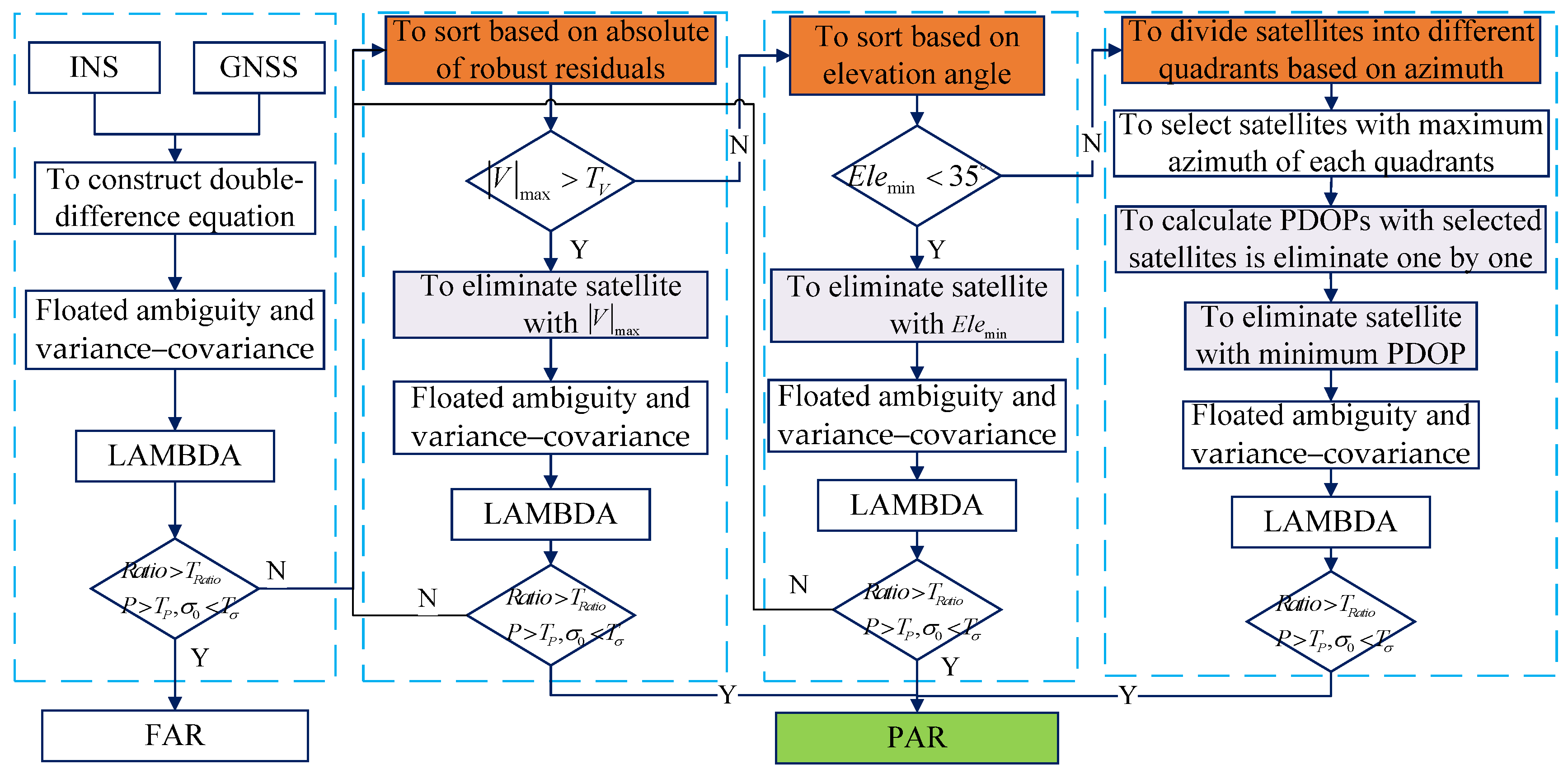
To evaluate the performance of the proposed PAR algorithm, five schemes of the SF GNSS RTK/INS for TC integration were designed, and self-development software was used to resolve these data. Scheme 1 is the FAR. Scheme 2 is the PAR based on the elevation angle (PARE). The satellites are sorted according to the elevation angle, and the satellites are eliminated one by one. Scheme 3 is the PAR based on the posteriori residual and elevation angle, and the posteriori residual is calculated without robust estimation (PARVNE). For scheme 3, the satellites are eliminated one by one if the absolute values of the posteriori residual are over the set threshold; otherwise, the satellites are successively eliminated based on the elevation angle. Scheme 4 is the PAR based on the robust posteriori residual and elevation angle (PARVYE), and the difference between scheme 3 and scheme 4 is that the posteriori residual is calculated using the robust estimation of the IGG-III. Scheme 5 is the proposed PAR based on the robust posteriori residual, elevation angle, and azimuth in the body plane frame (PARVYEO). The smoothing results of the GNSS RTK/INS for TC integration from Inertial Explorer 8.90 (IE) software were used as the reference.

3.1. Case One

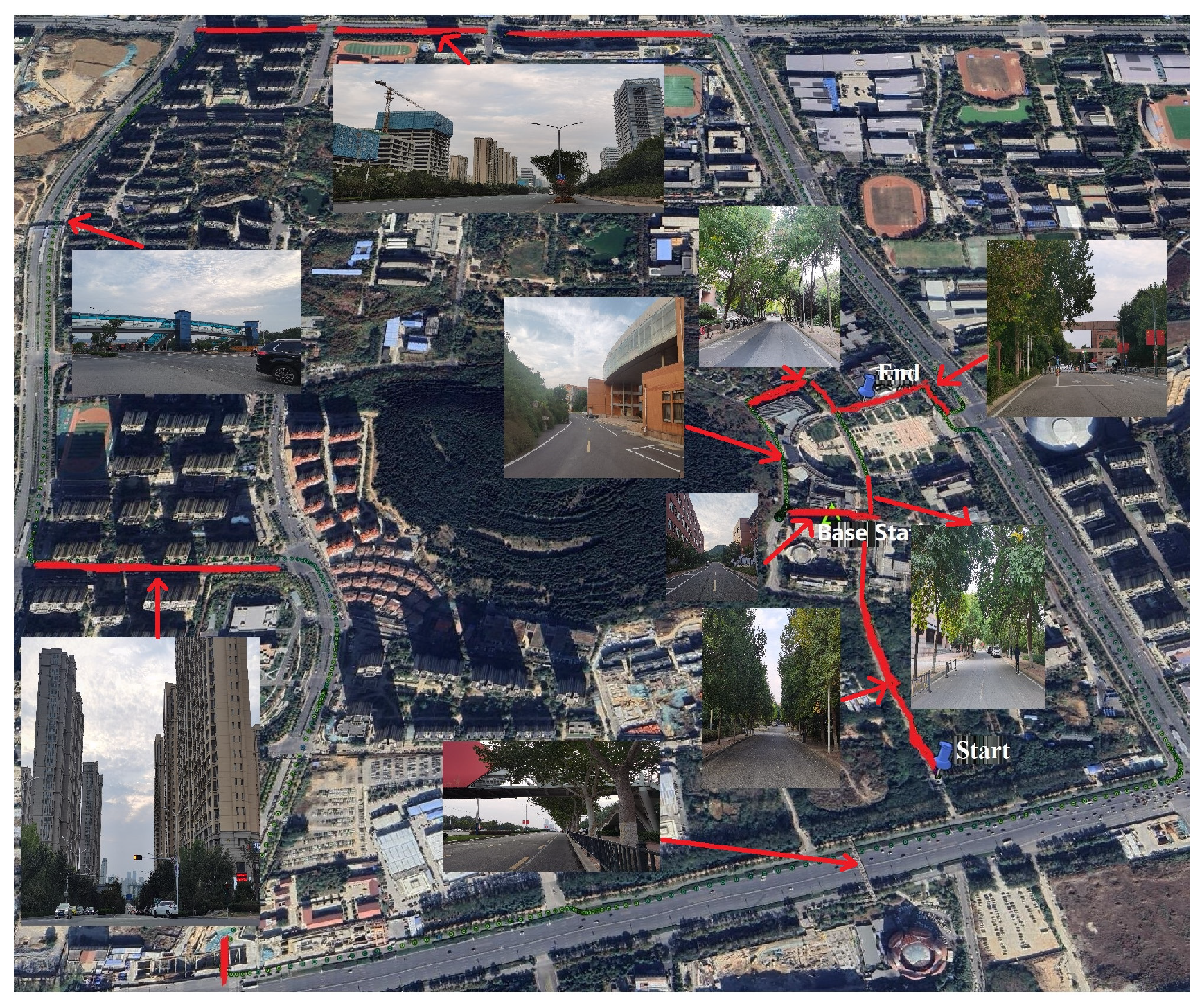
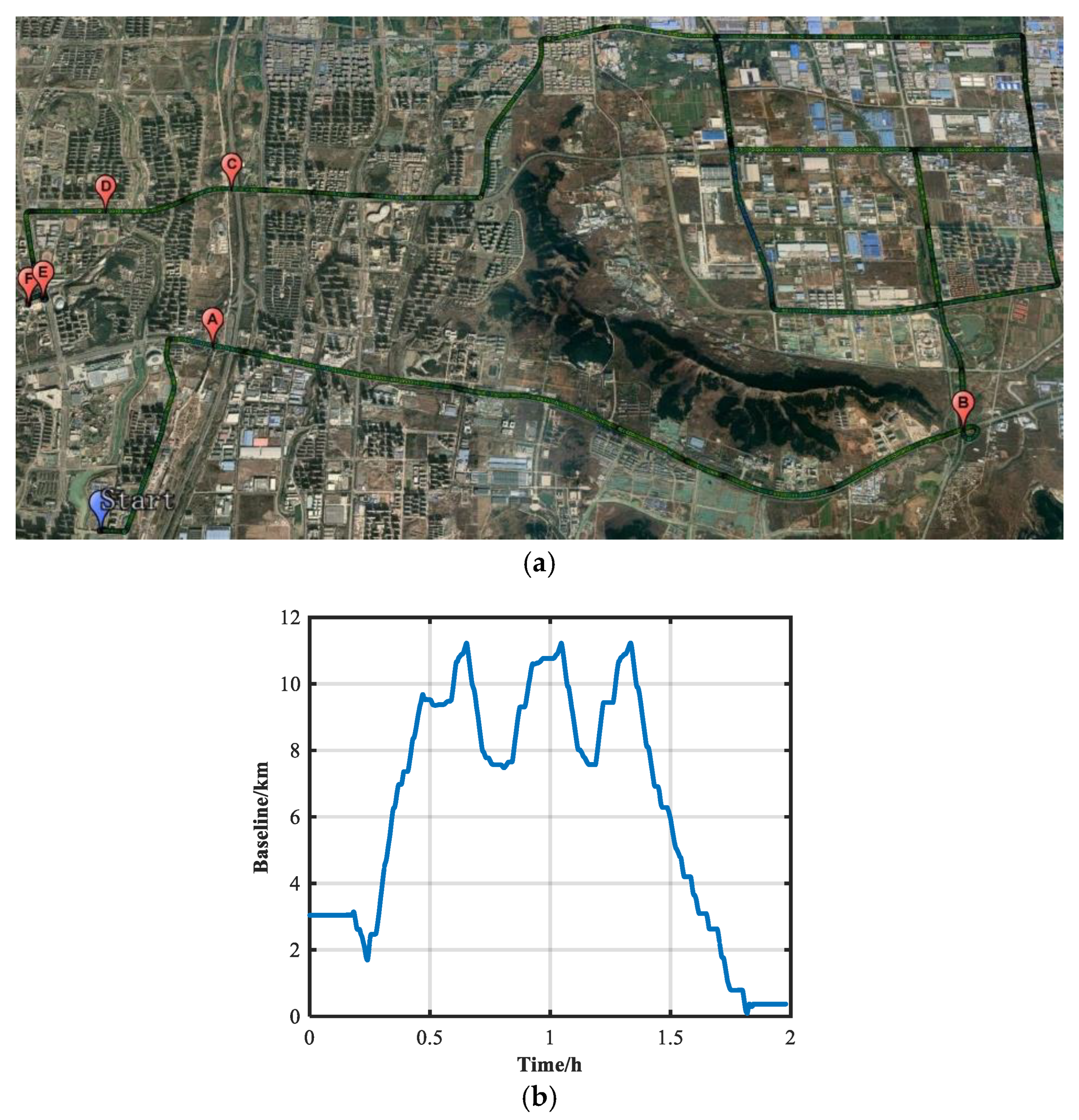
A CHCNAV receiver was set up on a roof as the base station, and the sample frequency was 1 Hz. The receivers on the base and rover stations could receive data from the GPS, BDS2, BDS3, and Galileo satellites. The data were collected in urban areas in Jinan, and GNSS-blocked environments such as tall buildings, dense trees, and viaducts were included in this experiment. Figure 6 shows the experimental areas and the length of the baseline. In Figure 6a, the areas marked A, B, C, D, E, and F are the selected GNSS-blocked environments, and the length of the baseline is over 10 km (Figure 6b).

Figure 7 shows the number of satellites and PDOP in the entire experimental area. In Figure 7a, the numbers of the GPS (G), BDS (C), and Galileo (E) satellites are greater than six, ten, and two, respectively; however, the number of satellites is much lower in the blocked environments, such as the environments marked in Figure 6a. In Figure 7b, the PDOP changes frequently during multiple periods, and the maximum value exceeds six.

The five designed schemes were used to solve this data to evaluate their performance.

Table 1. Average number of used satellites and PDOP for the designed schemes.

	PARE	PAREVN	PAREVY	PARVYEO
Number of satellites	27.13	27.52	27.47	27.59
PDOP	1.41	1.31	1.29	1.27

presents the average number of used satellites and the PDOP for the PARE, PAREVN, PAREVY, and PARVYEO schemes. The statistics of the FAR scheme are not presented because there are too few fixed solutions for this dynamic data. In Table 1, the proposed algorithm has the largest number of satellites (27.59), and there is 1.67% improvement in the number of satellites compared with the PARE algorithm. The proposed algorithm has the best geometry and the smallest PDOP (1.27), and the PDOP is improved by 9.93% compared to the PARE scheme.

In this study, the ratio of the fixed number of integer ambiguities to the total epoch number was used as the fixed rate of the integer ambiguity.

Table 2. Fixed rates and average numbers of the fixed ambiguities for the designed schemes.

	FAR	PARE	PARVNE	PARVYE	PARVYEO
Fixed rate	14.05%	98.92%	99.20%	99.24%	99.40%
Fixed number	/	24.24	24.58	24.46	24.61

presents the fixed rates of the integer ambiguities and the average numbers of fixed ambiguities for the FAR, PARE, PAREVN, PAREVY, and PARVYEO schemes. In Table 2, the fixed rate is only 14.05% for the FAR scheme. There are three possible reasons for the low fixed rate of the FAR scheme. First, the threshold of the SNR is set to 25 for data processing, and most of the epochs have low-quality satellites, which affects the fixed performance of the FAR scheme. Second, the predicted position by the INS is used to assist ambiguity resolution, and the error of the predicted position will be gradually accumulated when the INS works alone for a long time, and this large position error will affect the accuracy of the float AR. Third, the baseline is over 10 km at some moments, and the residual atmospheric error has a slight impact on the accuracy of the float AR. The fixed rate increases to 98.92% for the PARE scheme, and the fixed rate increases to 99.20% for PARVEN. When the robust estimation of IGG-III is used, the fixed rate is further improved. The fixed rate is 99.24% for PAREVY, and the fixed rate increases to 99.40% for PARVYEO. Among all of the AR schemes considered in this study, the proposed algorithm has the highest fixed rate. The statistics of the average number of fixed ambiguities for FAR are not presented because the epoch number of the fixed solution is too small. In Table 2, the average fixed number of integer ambiguities for PARVYEO is 24.61, and it is improved by 1.50%, 0.12%, and 0.61% compared to those of PARE, PAREVN, and PAREVY, respectively.

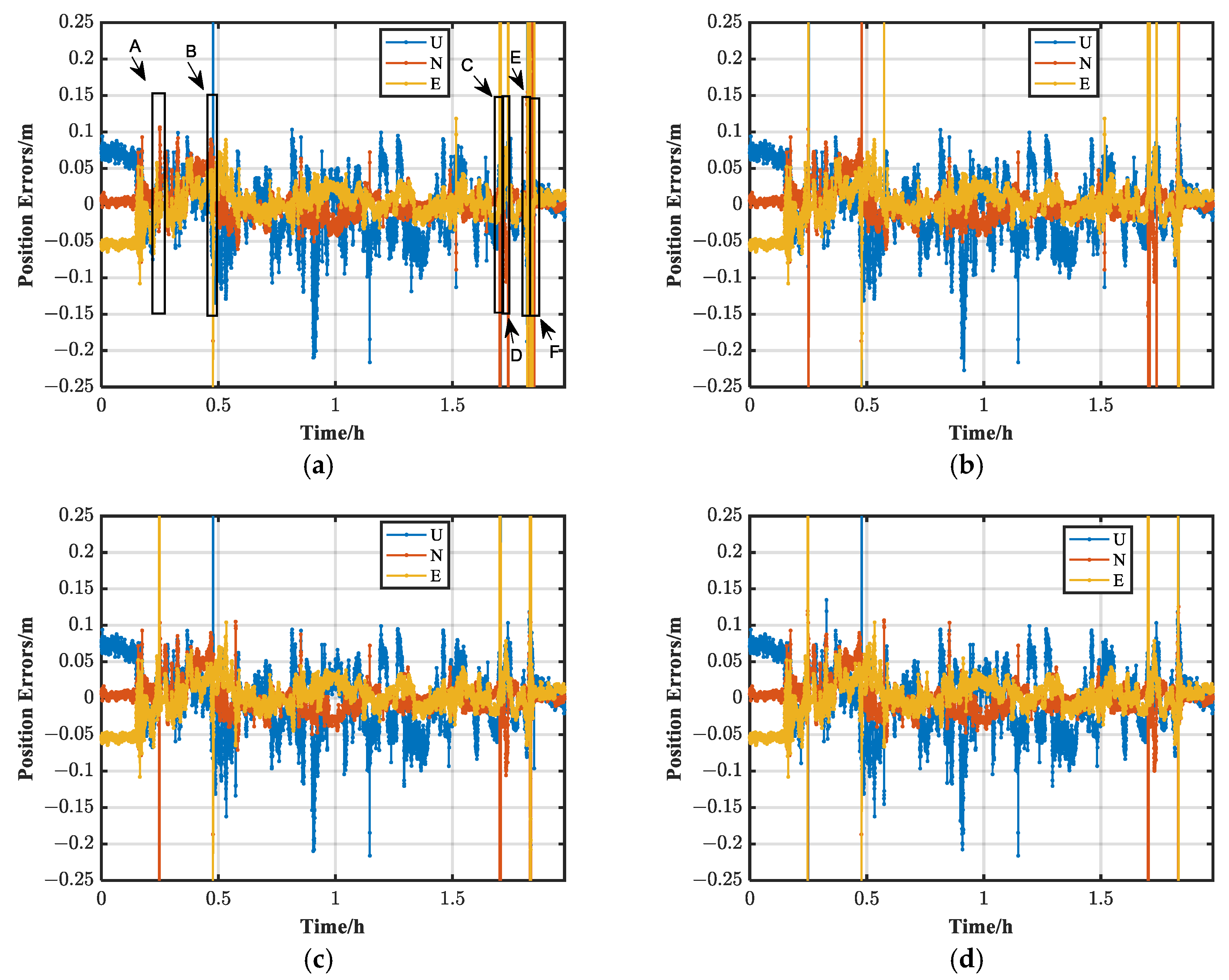
Figure 8 shows the position errors of the PARE, PAREVN, PAREVY, and PARVYEO schemes, and the areas marked A, B, C, D, E, and F in Figure 8a are the GNSS-blocked areas marked in Figure 6a. In this paper, only the results of the fixed ambiguity are counted. The positioning performance of FAR is not discussed because the fixed epoch is low. In Figure 8, the position errors of the PARE, PAREVN, PAREVY, and PARVYEO schemes are mostly at the centimeter level, and large errors exist at some timepoints. In Figure 8a, PARE does not have large errors in area A compared with the other PAR schemes. This is because area A is the scene of continuous viaducts, and the PARE scheme has more gap epochs than the other PAR schemes. In area A, the fixed rate is improved when PAREVN, PAREVY, and PARVYEO are used; however, the integer ambiguities are incorrectly fixed at some epochs. In areas B and C, the scenes are of a vertical transportation hub and viaduct, and all the PAR methods have large errors. In area D, which contains trees and buildings, there are large position biases for PARE and PAREVN, and the position results are significantly improved by PAREVY and PARVYEO. In area E, which contains the porch, dense trees, and tall buildings, the position results of PARE have continuous meter-level errors, and the other PAR schemes quickly converge to a centimeter-level positioning accuracy. In area F, which is the scene of a tall corridor, the position results of PARE have large errors, while the position results of the other PAR schemes are still at the centimeter level.

Table 3. The accuracy statistics of the position errors for the designed PAR schemes.

	PARE	PARVNE	PARVYE	PARVYEO
N (m)	0.94	0.27	0.34	0.22
E (m)	1.45	0.14	0.23	0.14
U (m)	0.90	0.45	0.38	0.40
3D (m)	1.95	0.54	0.56	0.48

is the RMS (Root Mean Square) statistics of the position errors for the designed PAR schemes shown in Figure 8. The positioning accuracies of these designed PAR schemes are on the decimeter level or meter level due to the influence of complex GNSS-blocked environments. In Table 3, the 3D RMS of the PARE scheme is 1.95 m, and the positioning accuracy is the lowest among all the designed PAR schemes. The RMSs of the PARVNE and PARVYE schemes are basically the same and outperform that of the PAR scheme. The RMS of the PARVYEO scheme is optimal, reaching 0.48 m. Compared with the PARE, PARVNE, and PARVYE schemes, the 3D RMS of the proposed scheme is improved by 75.49%, 12.09%, and 15.19%.

Figure 9 presents the cumulative probabilities of the 3D position error for the FAR, PARE, PAREVN, PAREVY, and PARVYEO schemes. In Figure 9, the cumulative probability of the 3D position error within 0.10 m is only 13.74% for the FAR scheme because of the low fixed rate of the integer ambiguities, and the cumulative probability is significantly increased to 95.34% by PARE. The cumulative probability of the 3D position error within 0.10 m reaches 96.43% for PAREVY, and the cumulative probability is the highest for the proposed PARVYEO algorithm (96.62%). The probability that the 3D position error is over 0.2 m is 0.88%, 0.75%, and 0.38% for the PARE, PARVNE, and PARVYE schemes, and it is only 0.31% for the proposed algorithm.

Table 4. The statistics of the computation time for the designed PAR schemes.

	PARE	PARVNE	PARVYE	PARVYEO
Computation times/s	146.575	148.920	151.626	152.549

shows the computation time of the designed PAR schemes, and the epoch numbers are 7124 for this data. In Table 4, the computation time is 146.575 s for the PARE scheme, and the computation time increases to 148.920 s and 151.626 s for the PARVNE and PARVYE schemes. Because the robust posterior residual, the elevation angle, and the azimuth in the body frame are used for the proposed scheme, the computation cost is the highest, reaching 152.549 s. Compared with the PARE scheme, the computation time is slightly increased by 4.08%. The average computation time of the proposed PAR scheme is 0.021 s for each epoch. Therefore, the proposed scheme still has great computational efficiency and can meet the requirements of real-time application in urban environments.

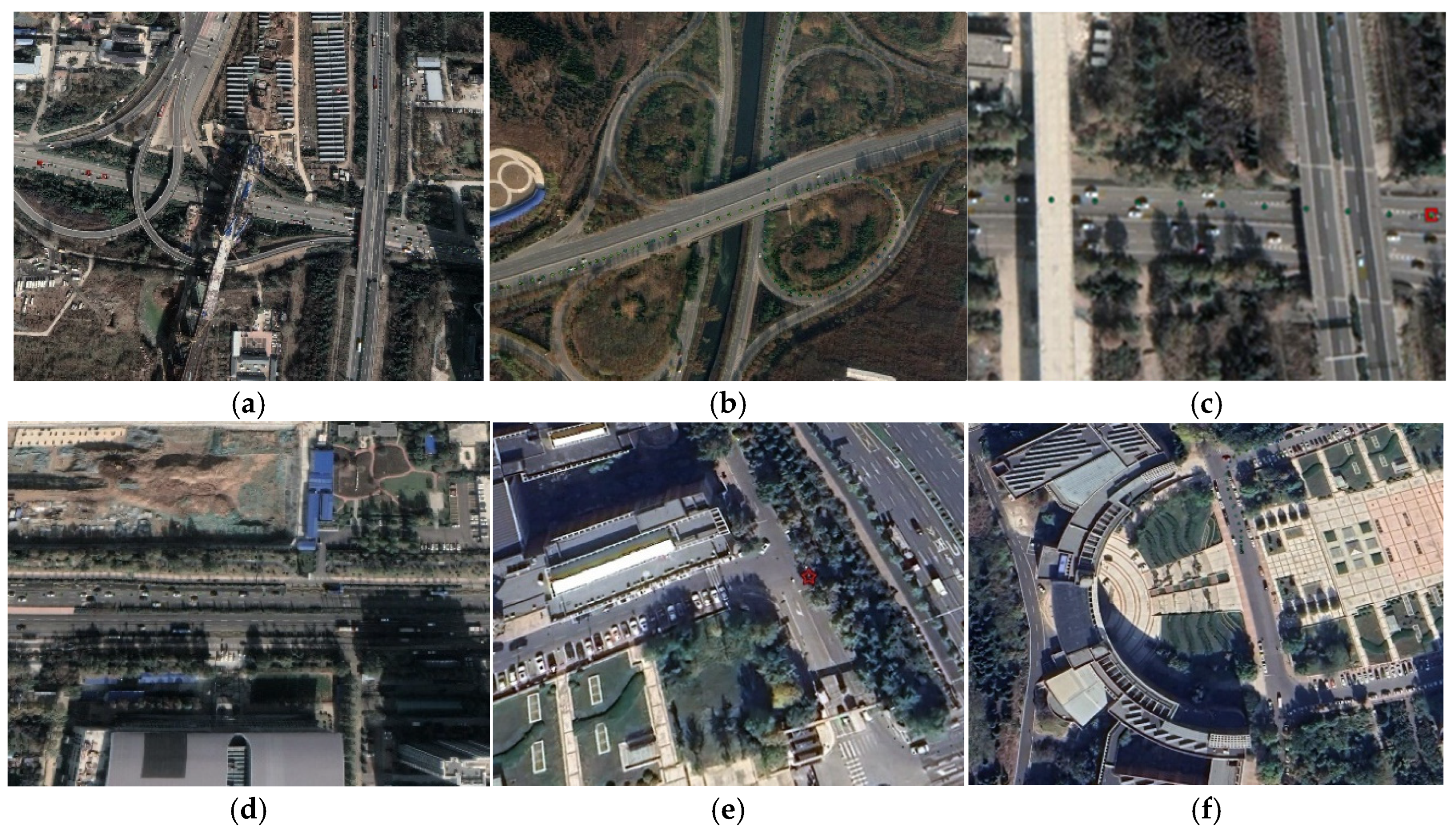
To evaluate the performance of the proposed algorithm in GNSS-blocked urban environments, the positioning performance of several PAR schemes in the six areas marked in Figure 6 is analyzed. Figure 10 shows the environments of the six marked areas. Figure 10a shows a mixed shielded environment, including a vertical transportation hub and two viaducts. Figure 10b shows a vertical transportation hub. Figure 10c shows the environment with two continuous viaducts. Figure 10d shows an environment with dense trees and tall buildings along the path. Figure 10e shows a continuous shielded environment containing a porch, a tree-lined road, and a tall building. Figure 10f shows an environment with tall buildings.

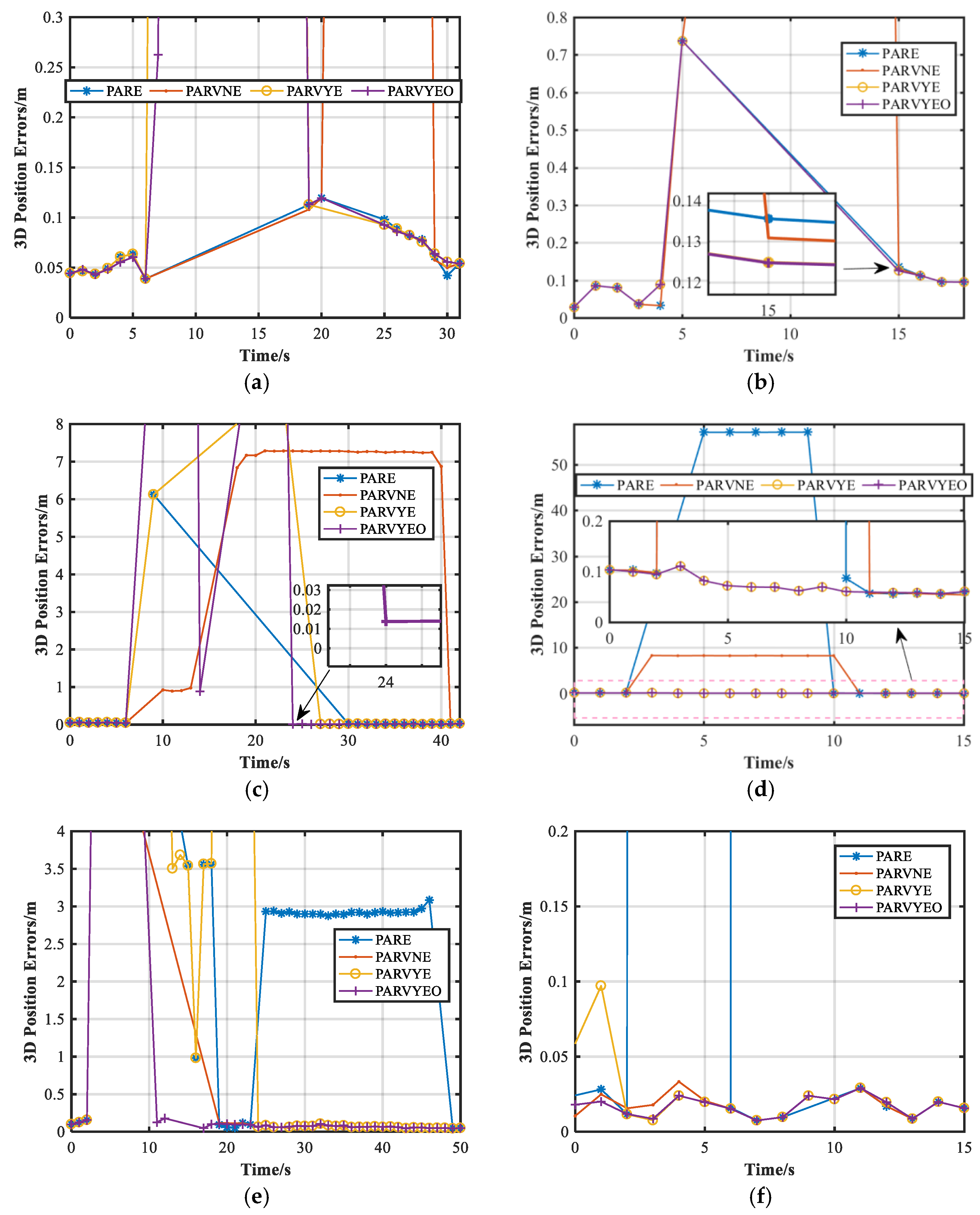
Figure 11 presents the position errors of the designed PAR schemes in the six marked areas. In Figure 11a, the ambiguities of several PAR schemes cannot be fixed for some time because of the serious GNSS blocking in this environment, and the epoch numbers of unfixed ambiguity for PARE, PARVNE, PARVYE, and PARVYEO are 16, 18, 16, and 10, respectively. The fixed rate of the proposed scheme in this GNSS-blocked environment is better than that of other PAR schemes. Although there are some epochs where ambiguities are incorrectly fixed for the PARVNE, PARVYE, and PARVYEO schemes, the position accuracy of the proposed scheme quickly converges to the centimeter level when the GNSS-blocked environment is passed. However, the centimeter-level positioning results can be obtained up until 29 s for the PARVNE scheme. In Figure 11b, the PARE, PARVNE, PARVYE, and PARVYEO schemes have decimeter-level positioning errors in the fifth second, which is because only four pairs of satellites are available in this epoch when the vehicle enters the vertical transportation hub. In this GNSS attenuation area, the epoch numbers of the unfixed ambiguities for the PARE, PARVNE, PARVYE, and PARVYEO schemes are 9, 8, 9, and 9, respectively. The PARVNE scheme has meter-level positioning errors when the vehicle exits the vertical transportation hub; however, the position accuracies of the PARVYE and PARVYEO schemes, which use the IGG-III, quickly converge to the centimeter level. In Figure 11c, the position errors of the designed PAR schemes are at the meter level when the vehicle enters the viaduct environment, and there are some epochs where the fixed solution of the integer ambiguity cannot be obtained. The epoch numbers of unfixed ambiguity for the PARE, PARVNE, PARVYE, and PARVYEO schemes are 22, 7, 16, and 11, respectively. In area C, the PARVNE scheme has the best fixed rate of integer ambiguity, followed by the proposed scheme. However, there are many epochs where the ambiguity is incorrectly fixed for the PARVNE scheme, and the centimeter-level positioning results can be obtained until the 41st second. The corrected integer ambiguity and centimeter-level solution can be obtained most quickly for the proposed algorithm when the vehicle passes the viaduct environment. In Figure 11d, the maximum position error of the PARE scheme reaches tens of meters, and the maximum position error is decreased to the meter level by the PARVNE scheme. The PARVYE and PARVYEO schemes can resist the influence of gross errors, and their position errors are at the centimeter level. In Figure 11e, the position errors of these PAR schemes reach the meter level due to the presence of the continuous complex environments shown in Figure 10e, and the epoch numbers of unfixed ambiguity for the PARE, PARVNE, PARVYE, and PARVYEO schemes are 6, 12, 5, and 5, respectively. The meter-level position error of the PARE scheme starts from the third second to the eighteenth second where there are porch and dense tree environments during this time. The meter-level position error also occurs for 22 s after the vehicle enters the tall building environment. For the PARVNE scheme, the centimeter-level position results can be obtained at the nineteenth second when the porch and dense tree environment are passed. For the PARVYE scheme, the meter-level position errors start at 3 s, and the centimeter-level position results can be obtained up until 25 s. However, the proposed algorithm can obtain the centimeter-level position results in the eleventh second. Therefore, the proposed algorithm has the fastest performance to converge to the centimeter-level position result among all the designed PAR schemes in this GNSS-blocked area. In Figure 11f, the position errors are tens of meters for the PARE scheme due to the obstruction of tall buildings, and the other PAR schemes can resist the influence of the gross error. In summary, the centimeter-level position results can be obtained most quickly by the proposed scheme compared to other PAR schemes in complex GNSS-blocked environments.

In these six areas of complex GNSS-blocked environments, the total epoch number is 177, and the epoch numbers of ambiguity fixing for the PARE, PARVNE, PARVYE, and PARVYEO schemes are 118, 131, 129, and 140. The fixed rates of the PARE, PARVNE, PARVYE, and PARVYEO schemes are 66.67%, 74.01%, 72.88%, and 79.10%, and the fixed rate of the proposed scheme is improved by 18.64%, 6.87%, and 8.53% compared to the PARE, PARVNE, and PARVYE schemes. The probability of the 3D position error within 0.10 m is 36.72%, 42.94%, and 55.32% for the PARE, PARVNE, and PARVYE schemes, which is improved to 60.45% by the proposed scheme.

Table 5. The statistics of the position errors for the designed PAR schemes in the six marked areas.

	PARE	PARVNE	PARVYE	PARVYEO
Median (m)	0.54	1.94	0.06	0.059
Mean (m)	5.55	1.85	2.27	1.02
RMS (m)	11.81	3.96	4.13	3.37

shows the statistics of the position errors for the PARE, PAREVN, PAREVY, and PARVYEO schemes in the above six areas. In Table 5, the proposed algorithm has the lowest average median and mean values of the 3D position errors, i.e., 0.059 m and 1.02 m, respectively. Compared with the PARE, PAREVN, and PAREVY schemes, the average value of the 3D median position errors of the proposed algorithm is improved by 89.05%, 96.98%, and 0.68%, respectively, and the average value of the 3D mean position error of the proposed algorithm is improved by 81.62%, 44.90%, and 55.13%, respectively. The RMSs of the PARE, PARVNE, PARVYE, and PARVYEO schemes are 11.81 m, 3.96 m, 4.13 m, and 3.37 m, respectively, and the proposed scheme has the highest positioning accuracy. Compared with other PAR schemes, the RMS of the 3D position error of the proposed scheme is improved by 71.56%, 14.88%, and 22.48%, respectively.

Therefore, the positioning performance of the proposed scheme is better than that of the other PAR schemes in complex GNSS-blocked areas, and the fixed rate of integer ambiguities is optimal among all the designed PAR schemes. The proposed algorithm also has the fastest performance to converge to the centimeter-level position result among all designed PAR schemes after the vehicle enters the GNSS-blocked environments.

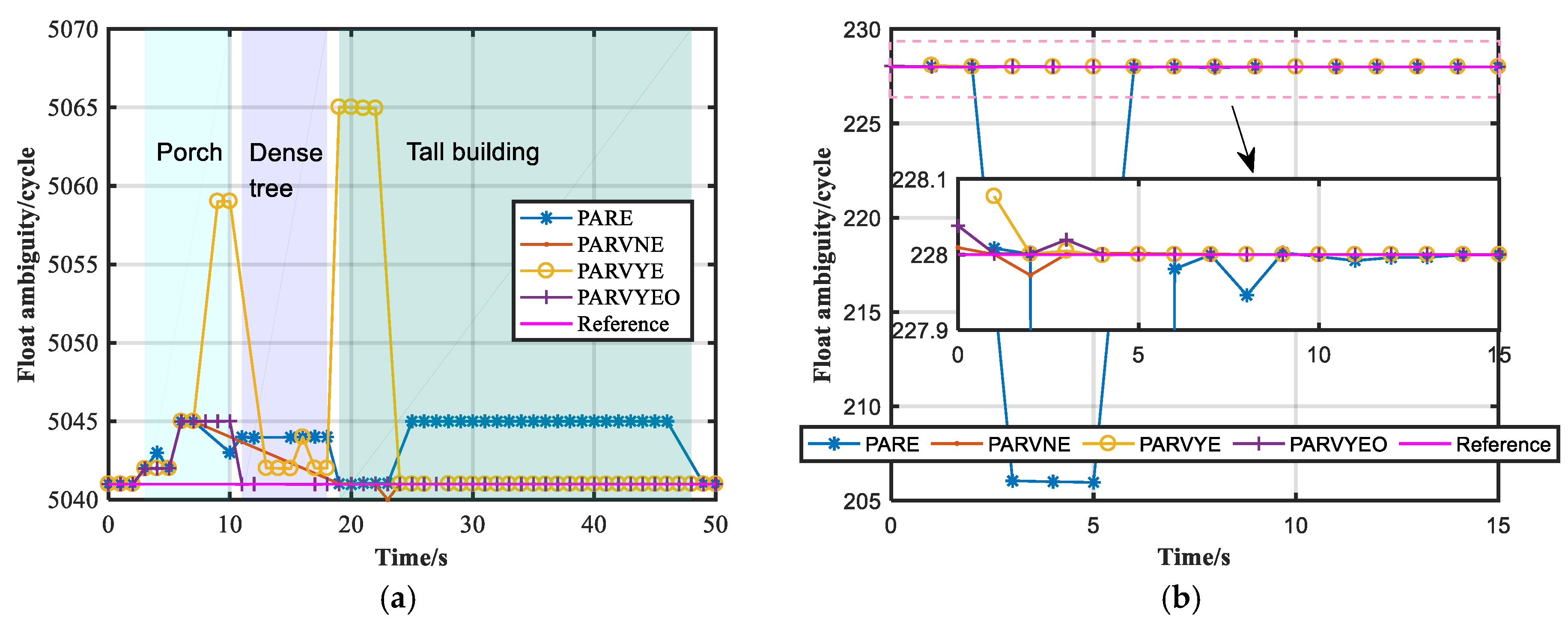
In all the epochs of areas E and F, the common satellite is present for these designed PAR schemes, and there are no continuous common satellites for the designed PAR schemes in areas A, B, C, and D. Therefore, area E and area F are used as an example to analyze the AR performance of these designed PAR schemes. Figure 12 shows the float ambiguity of the common satellite for these designed PAR schemes in areas E and F, and the pink line is the integer ambiguity reference. Figure 12a is the float ambiguity of common satellite G15 in area E. In Figure 12a, the shaded areas represent the area sheltered by the porch, dense trees, and tall buildings. The float ambiguity has a large bias for several PAR schemes after the vehicle enters the porch area in the third second, and the position results also have a large bias for every PAR scheme (Figure 11e). The PARE scheme is seriously affected by the gross errors, and the float ambiguity has a large bias in the GNSS-blocked areas of the porch and dense trees. In the tall building areas, the float ambiguity has a continuous bias that starts at 25 s, and the high-accuracy float ambiguity is obtained up until 49 s. For the PAREVN scheme, the data gap occurs after the seventh second, and the high-accuracy float ambiguity is solved at 19 s. The large bias of the PARVYE scheme starts at the third second, and the high-accuracy float ambiguity is solved at 24 s. For the proposed algorithm, when the vehicle passes the porch environment, the reliable float ambiguity is obtained at 11 s. The data gap occurs after the thirteenth second during passage through the environment of dense trees, and the high-accuracy float ambiguity is obtained when the vehicle passes the environment of dense trees at the eighteenth second for the proposed scheme. Therefore, the proposed algorithm can most quickly obtain the high-accuracy float ambiguity in the multiple GNSS-blocked environments. Figure 12b is the float ambiguity of common satellite G05 in area F, and the area is sheltered by tall buildings. In Figure 12b, the float ambiguity has a large bias that is about 22 cycles for the PARE scheme from the third second to the fifth second, and the continuous high-accuracy float ambiguity can be obtained for the PAVNE, PARVYE, and PARVYEO schemes. In the single GNSS-blocked environment of tall buildings, the proposed algorithm can obtain a stable and high-accuracy float ambiguity.

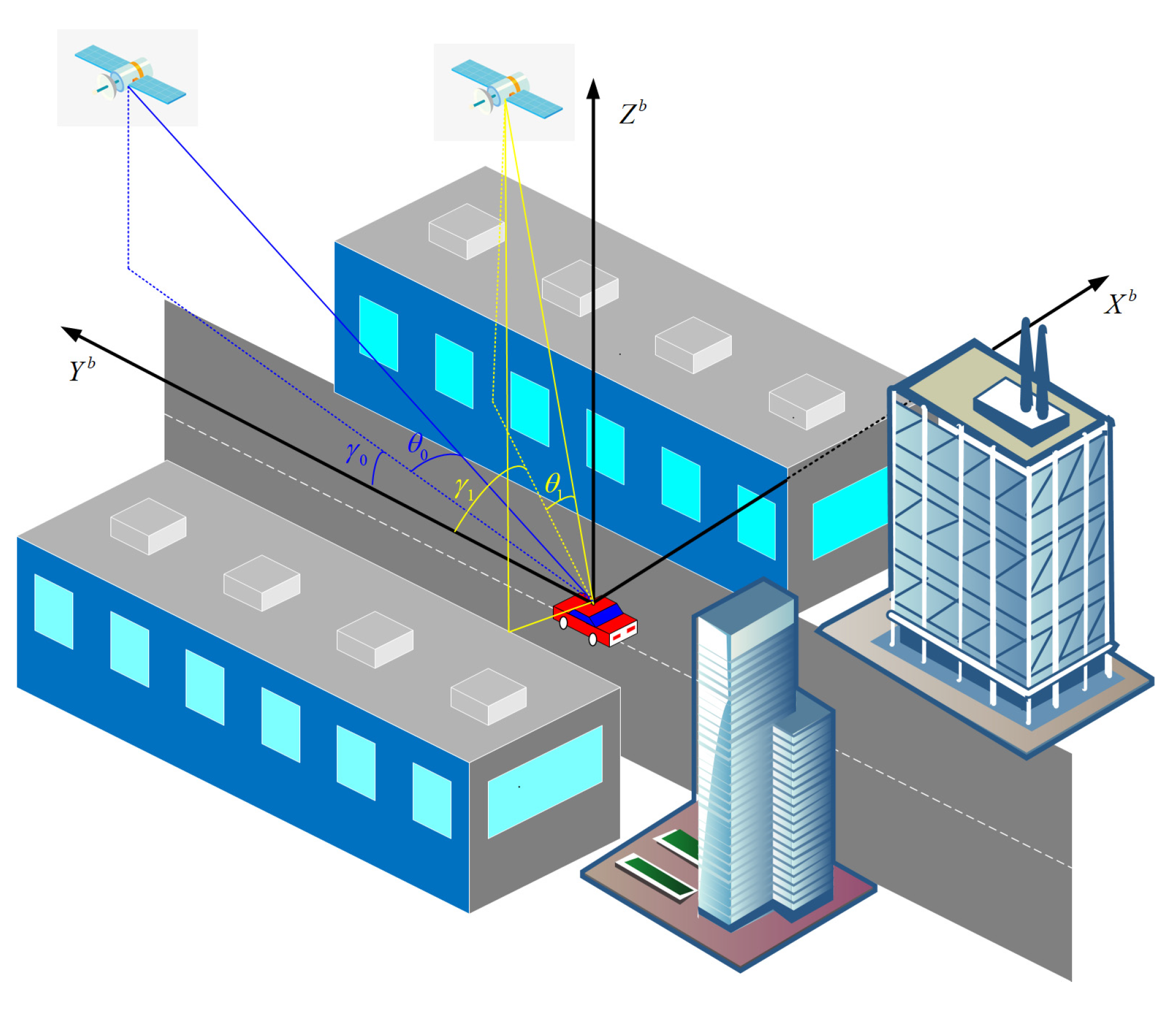
Figure 13 shows the sky plot of the satellites in the body frame for the seventeenth second shown in Figure 12a. At this time, the vehicle reaches the position of the red pentagram in Figure 10e, and only the proposed PAR algorithm can fix the ambiguities. In Figure 13, F, B, L, and R denote the forward, backward, left, and right directions of the road, respectively. 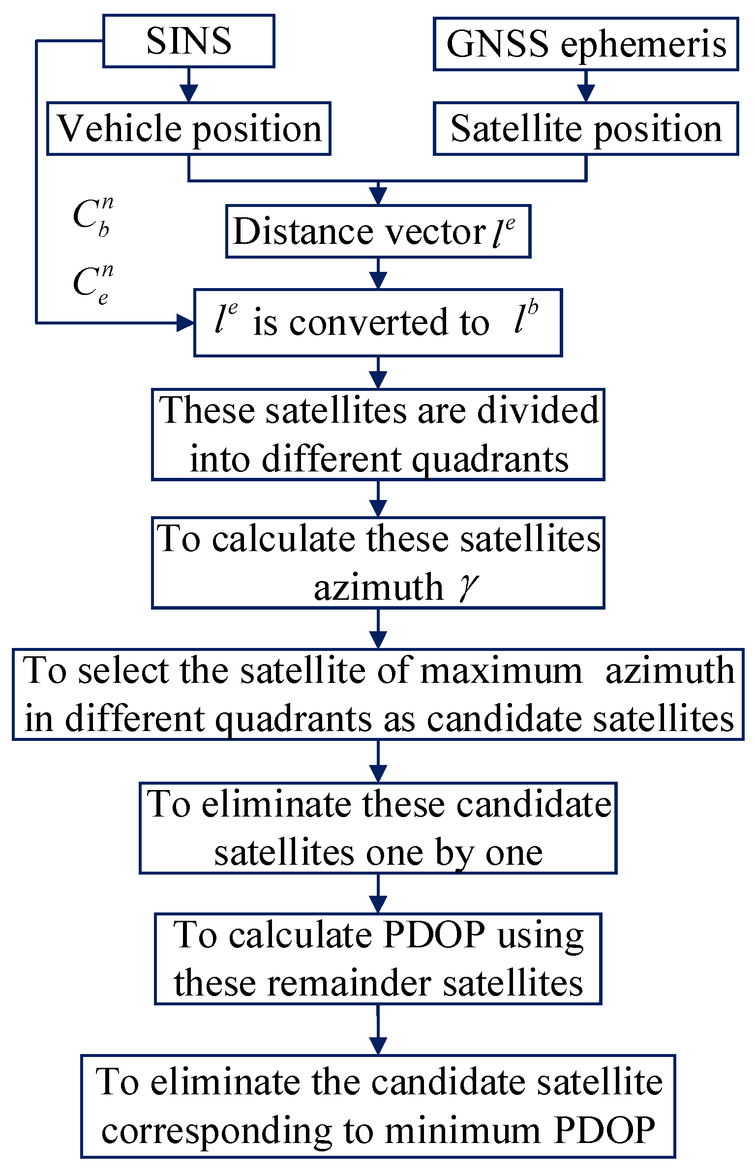In Figure 13a, there are fewer visual satellites on the two sides of the road, and as can be seen from Figure 10e, this is because tall buildings and dense trees are located on both sides of the road. Due to the more severe GNSS-blocked environment on the right side of the road, the quality of the visual satellite in this area is low. Visual satellites C01, C13, and C59 in the forward and backward parts of the road are of high quality, and their SNRs are all greater than 37. Therefore, the satellite selection strategy based on the azimuth in the body plane frame is possible. When the proposed algorithm is used to select the subset of satellites, C06, C16, C14, C60, and G11 are successively eliminated based on the elevation angle, and G05, C08, G29, C27, and E15 are eliminated one by one based on the azimuth in the body plane frame. The ambiguity of the remaining satellite (Figure 13b) can be fixed. In Figure 13b, the satellites in the forward and backward directions are used, and the low-quality satellites on both sides of the road are eliminated.

In summary, the proposed algorithm has the best ability to resist gross errors in GNSS-blocked environments, and the proposed algorithm can achieve centimeter-level positioning faster than the other PAR schemes.

3.2. Case Two

A dynamic dataset of short baseline values, which included multiple GNSS-blocked environments, was collected by the vehicle-borne system. The data was collected in urban areas in Jinan, and the GNSS-blocked environments include tall buildings, dense trees, and pedestrian overpasses in these experiment areas. Figure 14 shows the experimental areas and GNSS-blocked environments. In Figure 14, the red line represents the GNSS-blocked area, and the red arrow points to the location of GNSS-blocked environment. The receivers of the base and rover stations could receive data from the GPS, BDS2, and Galileo satellites, and the baseline is within 2 km.

Figure 15 shows the number of satellites and PDOP in the entire experimental area. The satellite number changes frequency due to multiple GNSS-blocked environments in this data, and the PDOP is poor when the satellite is blocked.

These five designed schemes were used to solve this data to evaluate the performance of the proposed schemes.

Table 6. Fixed rates of the integer ambiguities for the designed schemes.

	FAR	PARE	PARVNE	PARVYE	PARVYEO
Fixed rate	67.84%	96.17%	97.55%	97.99%	98.74%

is the fixed rate of the integer ambiguities for the five designed schemes. In Table 6, the fixed rate of the FAR scheme is 67.84% in the GNSS-blocked environments. The fixed rates are increased to 96.17%, 97.55%, and 97.55% by the PARE, PARVNE, and PARVYE schemes, respectively. The proposed scheme has the best fixed rate, reaching 98.74%.

Figure 16 shows the position errors of the designed schemes, and only the position results of fixed ambiguity are counted. In Figure 16, there are meter-level position errors for the five schemes due to multiple GNSS-blocked environments. In Figure 16a, there are meter-level position errors for some epochs, and data gaps also occur for some epochs because the ambiguities are unfixed. The epoch number of these fixed ambiguities is increased by the designed PAR schemes. Compared with the PARE, PARVNE, and PARVYE schemes, the epoch number of the meter-level position errors of the proposed scheme is significantly reduced, and the proposed scheme has a better ability to resist gross errors than the other designed PAR schemes.

Table 7. The accuracy statistics of the position errors for the designed schemes.

	FAR	PARE	PARVNE	PARVYE	PARVYEO
N (m)	0.72	0.76	0.64	0.67	0.63
E (m)	0.55	0.62	0.89	0.56	0.46
U (m)	1.15	1.51	0.78	1.36	0.74
3D (m)	1.46	1.80	1.35	1.61	1.07

shows the RMS statistics of the position errors for the designed schemes. In Table 7, the position accuracy is at the meter level for the designed schemes, and the RMS of the position errors for the proposed scheme is the optimal compared to the other designed schemes. The RMS of the position errors for the proposed scheme is 0.63 m, 0.46 m, and 0.74 m in the N, E, and U directions, respectively, and the RMS of the 3D position error reaches 1.07 m. Compared with the FAR, PARE, PARVNE, and PARVYE schemes, the RMS of the 3D position error of the proposed scheme is improved by 26.70%, 40.51%, 20.56%, and 33.47%.

Figure 17 shows the cumulative probability of the 3D position errors for the designed schemes. In Figure 17, the cumulative probability of the 3D position errors within 0.1 m is 32.35% for the FAR scheme, and the cumulative probabilities are increased to 47.86%, 45.04%, and 45.98% by the PARE, PARVNE, and PARVYE schemes. The highest cumulative probability is obtained by the proposed scheme, and the probability reaches 50.00%. The cumulative probability within 0.2 m reaches 64.01% for the FAR scheme, and the cumulative probability is increased to more than 80% for the designed PAR scheme. The proposed scheme has the highest cumulative probability, reaching 92.59%.

For this short-baseline data of multiple GNSS-blocked environments, the proposed scheme obtains the highest fixed rate of integer ambiguity and the best positioning accuracy compared to other designed schemes.

4. Conclusions

Reliable and correct integer ambiguity is key to obtaining high-accuracy positioning. In complex urban environments, SF GNSS observations are susceptible to interference, which leads to the unreliable AR. In this study, we developed a sequential PAR strategy based on the robust posteriori residual, elevation angle, and azimuth in the body plane frame. The performance of the proposed algorithm was analyzed using dynamic vehicle-borne data in complex urban environments. The fixing rates of the FAR scheme for these two data were only 14.05% and 67.84%, and the proposed PAR algorithm had the highest fixing rate (99.40% and 98.74%). For the first dynamic data, the cumulative probability of the 3-D position error within 0.10 m was only 12.74% for the FAR scheme, and the cumulative probability of the 3D position error within 0.10 m was the highest for the proposed algorithm (96.62%). The proposed algorithm had the best positioning performance for the six GNSS-blocked environments analyzed in this study. For the second dynamic data, the proposed PAR algorithm had the highest fixing rate, and the positioning accuracy of the 3D position error for the proposed scheme was improved by 26.70%, 40.51%, 20.56%, and 33.47% compared to the FAR, PARE, PARVNE, and PARVYE schemes.

References

1. Xi, R.J.; Xu, D.S.; Jiang, W.P.; He, Q.Y.; Zhou, X.H.; Chen, Q.S.; Fan, X.C. Elimination of GNSS carrier phase difraction error using an obstruction adaptive elevation masks determination method in a harsh observing environment. GPS Solut. 2023, 27, 139–154. [Google Scholar] [CrossRef]
2. Chai, D.S.; Ning, Y.P.; Wang, S.L.; Sang, W.G.; Xing, J.P.; Bi, J.X. A robust algorithm for multi-GNSS precise positioning and performance analysis in urban environments. Remote Sens. 2022, 14, 5155. [Google Scholar] [CrossRef]
3. Chai, D.S.; Chen, G.L.; Wang, S.L.; Lu, X.S. A New Single-Epoch Method for Resolving GNSS Ambiguity with Segmented Search in short baseline. Adv. Space Res. 2018, 62, 30–43. [Google Scholar] [CrossRef]
4. Xin, S.M.; Geng, J.H.; Zhang, G.H.; Ng, H.F.; Guo, J.; Hsu, L.T. 3D-mapping-aided PPP-RTK aiming at deep urban canyons. J. Geod. 2022, 96, 78–96. [Google Scholar] [CrossRef]
5. Li, H.Y.; Nie, G.G.; Wang, J.; Wu, S.G.; He, Y.F. A novel partial ambiguity method for multi-GNSS real-time kinematic positioning. J. Navig. 2021, 75, 1–14. [Google Scholar] [CrossRef]
6. Li, Z.; Xu, G.L.; Guo, J.; Zhao, Q.L. A sequential ambiguity selection strategy for partial ambiguity resolution during RTK positioning in urban areas. GPS Solut. 2022, 26, 92–107. [Google Scholar] [CrossRef]
7. Brack, A.; Gunther, C. Generalized integer aperture estimation for partial GNSS ambiguity fixing. J. Geod. 2014, 88, 479–490. [Google Scholar] [CrossRef]
8. Teunissen, P.J.G.; Joosten, P.; Tiberius, C.C.J.M. Geometry-Free ambiguity success rates in case of partial fixing. In Proceedings of the 1999 National Technical Meeting of the Institute of Navigation, San Diego, CA, USA, 25–27 January 1999; pp. 201–207. [Google Scholar]
9. Jiang, Y.; Ding, W.; Gao, Y.T.; Gao, Y. A new partial ambiguity resolution method based on modified solution separation and GNSS epoch-differencing. J. Geod. 2022, 96, 88–102. [Google Scholar] [CrossRef]
10. Teunissen, P.J.G.; Odolinski, R.; Odijk, D. Instantaneous BeiDou+GPS RTK positioning with high cut-off elevation angles. J. Geod. 2014, 88, 335–350. [Google Scholar] [CrossRef]
11. Parkins, A. Increasing GNSS RTK availability with a new single-epoch batch partial ambiguity resolution algorithm. GPS Solut. 2011, 15, 391–402. [Google Scholar] [CrossRef]
12. Dong, Y.; Zhang, Z.T.; Pang, L.L.; Dong, H.C.; Shi, Y.X. Partial ambiguity resolution considering the multipath effects in a canyon environment. Surv. Rev. 2024, 56, 300–315. [Google Scholar] [CrossRef]
13. Hsu, L.T. Analysis and modeling GPS NLOS effect in highly urbanized area. GPS Solut. 2018, 22, 7–18. [Google Scholar] [CrossRef]
14. Shi, J.B.; Gao, Y. A Fast Integer Ambiguity Resolution Method for PPP. In Proceedings of the 25th International Technical Meeting of the Satellite Division of The Institute of Navigation, Nashville, TN, USA, 17–21 September 2012; pp. 3728–3734. [Google Scholar]
15. Li, P.; Zhang, Z.H. Precise point positioning with ambiguity fixing. Sensors 2015, 15, 13627–13653. [Google Scholar] [CrossRef]
16. Wang, J.; Feng, Y. Reliability of partial ambiguity fixing with multiple GNSS constellations. J. Geod. 2013, 87, 1–14. [Google Scholar] [CrossRef]
17. Odijk, D.; Teunissen, P.J.G. ADOP in closed form for a hierarchy of multi-frequency single-baseline GNSS models. J. Geod. 2008, 82, 473–492. [Google Scholar] [CrossRef]
18. Zhang, C.L.; Chen, W.; Dong, D.N.; Kubo, N.; Wu, J.P. Application of optimal stopping theory in batch partial ambiguity resolution. GPS Solut. 2023, 27, 121–134. [Google Scholar] [CrossRef]
19. Liu, Y.; Gao, Z.Z.; Xu, Q.Z.; Li, Y.; Chen, L. Assessing partial ambiguity resolution and WZTD-constraint multi-frequency RTK in an urban environment using new BDS signals. GPS Solut. 2022, 26, 88. [Google Scholar] [CrossRef]
20. Man, X.S.; Dai, W.J.; Yu, W.K.; Jiang, Y.X.; Li, L.; Liu, Y. A TDCP-assisted partial ambiguity resolution method for GNSS Real-time kinematic positioning in challenging environment. GPS Solut. 2025, 29, 140–151. [Google Scholar] [CrossRef]
21. Liu, W.K.; Li, J.L.; Zeng, Q.; Guo, F.; Wu, R.P.; Zhang, X.H. An improved robust Kalman filtering strategy for GNSS kinematic positioning considering small cycle slips. Adv. Space Res. 2019, 63, 2724–2734. [Google Scholar] [CrossRef]
22. Chai, D.S.; Sang, W.G.; Chen, G.L.; Ning, Y.P.; Xing, J.P.; Yu, M.W.; Wang, S.L. A novel method of ambiguity resolution and cycle slip processing for single-frequency GNSS/INS tightly coupled integration system. Adv. Space Res. 2022, 69, 359–375. [Google Scholar] [CrossRef]
23. Wen, Y.; Dai, W.; Yu, W.; Pan, L. Mitigation of multiple outliers using consistency checking for GNSS standard point positioning in urban areas. Adv. Space Res. 2023, 73, 1721–1733. [Google Scholar] [CrossRef]
24. Gu, Y.; Hsu, L.T.; Kamijo, S. GNSS/Onboard inertial sensor integration with the aid of 3-D building map for lane-level vehicle self-localization in urban canyon. IEEE Trans. Veh. Technol. 2016, 65, 4274–4287. [Google Scholar] [CrossRef]
25. Yin, J.; Li, T.; Yu, W.X.; Zou, D.P. Sky-GVINS: A sky-segmentation aided GNSS-Visual-Inertial system for robust navigation in urban canyons. Geo-Spat. Inf. Sci. 2024, 27, 2257–2267. [Google Scholar] [CrossRef]
26. Han, H.Z.; Wang, J.; Wang, J.L.; Moraleda, A.H. Reliable partial ambiguity resolution for single-frequency GPS/BDS and INS integration. GPS Solut. 2017, 21, 251–264. [Google Scholar] [CrossRef]
27. Li, T.; Zhang, H.P.; Gao, Z.Z.; Niu, X.J.; El-sheimy, N. Tight fusion of a monocular camera, MEMS-IMU, and single-frequency multi-GNSS RTK for precise navigation in GNSS-challenged environments. Remote Sens. 2019, 11, 610–632. [Google Scholar] [CrossRef]
28. Yang, Y.X.; Song, L.; Xu, T.H. Robust estimator for correlated observations based on bifactor equivalent weights. J. Geod. 2002, 76, 353–358. [Google Scholar] [CrossRef]
29. Wang, S.L.; Deng, J.; Ou, J.K.; Nie, W.F. Three-step Algorithm for Rapid Ambiguity Resolution between Reference Stations within Network RTK. J. Navig. 2016, 69, 1310–1324. [Google Scholar]
Figure 1. Narrow and long scenes.
Electronics 14 02712 g001
Figure 2. Body plane frame.
Electronics 14 02712 g002
Figure 3. Workflow of the satellite selection based on the azimuth in the body plane frame.
Electronics 14 02712 g003
Figure 4. Workflow of the proposed PAR strategy.
Electronics 14 02712 g004
Figure 5. Integrated navigation system of the Bynav A1-3L.
Electronics 14 02712 g005
Figure 6. Experiment areas and baseline length: (a) experiment areas; (b) baseline length.
Electronics 14 02712 g006
Figure 7. Number of satellites and PDOP of the data of case one: (a) number of satellites; (b) PDOP.
Electronics 14 02712 g007
Figure 8. Position errors of the designed PAR schemes; (a) PARE scheme; (b) PARVNE scheme; (c) PARVYE scheme; and (d) PARVYEO scheme.
Electronics 14 02712 g008
Figure 9. Cumulative probability of the position errors of the designed schemes.
Electronics 14 02712 g009
Figure 10. GNSS-blocked environments of the six marked areas: (a) area A; (b) area B; (c) area C; (d) area D; (e) area E; and (f) area F.
Electronics 14 02712 g010
Figure 11. Position errors of the six marked areas for the PARE, PARVNE, PARVYE, and PARVYEO schemes: (a) area A; (b) area B; (c) area C; (d) area D; (e) area E; and (f) area F.
Electronics 14 02712 g011
Figure 12. Float ambiguity of the common satellite for the designed PAR schemes in areas E and F: (a) float ambiguity of the common satellite G15 in area E; (b) float ambiguity of the common satellite G05 in area F.
Electronics 14 02712 g012
Figure 13. The sky plot of the satellites in the body frame: (a) sky plot of visible satellites; (b) sky plot of satellites for fixed ambiguity.
Electronics 14 02712 g013
Figure 14. Experiment areas and GNSS-blocked environments.
Electronics 14 02712 g014
Figure 15. Number of satellites and PDOP of the data of case two: (a) number of satellites; (b) PDOP.
Electronics 14 02712 g015
Figure 16. Position errors of these designed schemes: (a) FAR scheme; (b) PARE scheme; (c) PAREVN scheme; (d) PAREVY scheme; and (e) PARVYEO scheme.
Electronics 14 02712 g016
Figure 17. Cumulative probability of the 3D position errors for the FAR, PARE, PARVNE, PARVYE, and PARVYEO schemes.
Electronics 14 02712 g017