Abstract
To address the dual challenges of achieving high classification accuracy and real-time performance when detecting abnormal traffic in cloud environments, this study introduces an improved lightweight real-time detection model, IM-MobileNetV3. By standardizing features, dividing time windows, mapping spatially, and reshaping images, the model converts traffic features into 224 × 224 × 3RGB images, enabling multi-angle representation of traffic features and adapting to the model’s input requirements. Additionally, the MobileNet-Small model is improved by introducing the ECA module to replace the original SE module, avoiding the information loss that is often caused by channel dimension reduction, and the initial convolutional layer, bottleneck layer, and tail structure are optimized to enhance the feature extraction capability. The experimental results show that, on the CIC-IDS2018 dataset, IM-MobileNetV3 achieves an accuracy rate of 96.9%, reduces the number of parameters by 33% compared to the original model, and has a single-sample inference time of only 2.8 ms, significantly outperforming mainstream models.
1. Introduction
As cloud computing continues to develop, the intelligent transformation of network infrastructure accelerates. Network traffic exhibits complex characteristics such as high-dimensional heterogeneity, dynamic evolution, and nonlinear correlations, presenting increasingly severe security threats to cloud platforms, including common Distributed Denial of Service (DDoS) attacks and malicious web-crawlers. According to the “2023 Global DDoS Attack Status and Trend Analysis Report” [1], in 2023 the frequency of global DDoS attacks increased by 42%, with the proportion of ultra-large-scale attacks exceeding 1 Tbps, rising by 19%. Such attacks often occur within seconds. According to the DDoS report [2] released by Cloudflare, it defended against over 21.3 million DDoS attacks in 2024, with 420 ultra-large-scale attacks recorded in the fourth quarter alone. These attacks place increasing demands on the real-time performance and accuracy of traditional defense systems.
The current methods for detecting abnormal traffic can be categorized into two main types: the traditional machine learning-based approach (e.g., SVM [3] and random forest [4]), which requires manual feature engineering to extract the statistical characteristics of traffic, and cannot accurately represent all feature information; and the deep learning-based approach (e.g., ResNet [5], LSTM [6], and CNN [7]), which can capture deeper features of traffic. However, these models face challenges due to their large number of parameters, high computational complexity, and significant inference latency, making them unsuitable for the millisecond-level real-time requirements of cloud computing. Some researchers have proposed using the lightweight MobileNetV3 [8] for image classification, as it can improve accuracy while reducing inference latency. However, since MobileNetV3 is designed to be applied to natural images, it may not be suitable for traffic detection tasks.
In response to the above problems, this study improves the lightweight network architecture MobileNetV3-Small. In the second section of the paper, a comprehensive review of the current research status in the related field is conducted, alongside a detailed analysis of the deficiencies of previous achievements in the application of traffic detection, which provide clarification on the entry point of this study. In the third section, the research methods are expounded; the IM-MobileNetV3 model designed in this study is introduced and its advantages explained. Relevant experiments are conducted in the fourth section for proof. Finally, the fifth section provides a summary and outlook, along with suggestions for future expansion. Theoretically, it overcomes the adaptability bottleneck of the existing methods in the complex traffic scenarios that arise in the cloud environment and provides a deployable high-precision, real-time detection solution for the cloud platform. Some of the study’s core innovations are listed below:
- (1)
- A four-stage flow-image transformation mechanism is designed to enhance spatiotemporal pattern analysis ability through mirror filling and multi-channel gradient feature enhancement;
- (2)
- The Efficient Channel Attention (ECA) attention mechanism is adopted to optimize the feature weight allocation, and one-dimensional convolution is used instead of Multilayer Perceptron (MLP) to improve the efficiency;
- (3)
- The model hierarchy is reconstructed, the initial receptive field is expanded, redundant channels are compressed, and global average pooling (GAP) and global maximum pooling (GMP) dual-channel pooling are introduced to improve the tail feature extraction ability; and
- (4)
- The transfer learning strategy and prior knowledge of ImageNet are combined to accelerate the convergence of the model.
2. Related Works
In the face of complex traffic scenarios in a cloud environment, existing research faces core challenges such as insufficient feature representation ability, limited real-time performance, and poor model generalization.
Traditional machine learning methods, which manually mine the statistical characteristics of traffic, such as packet size, time intervals, protocol types, spatiotemporal correlations, and local feature distributions, are relatively weak. For instance, in [9], Dynamic Principal Component Analysis (DPCA) was used to extract traffic features and the covariance matrix was utilized to linearly expand feature data into vectors, making it difficult to detect short-term traffic mutations and other nonlinear attacks. Huang et al. [10] proposed a detection method based on Hidden Markov Models (HMMs), which calculates the statistical features of traffic, but fails to effectively analyze spatiotemporal correlations and local feature distributions. Ramprasath et al. [11] developed an anomaly detection model based on random forests (RFs) for cloud environments. Although the model’s structure is relatively simple, it divides decision trees by single features as thresholds, making it difficult to capture the synergistic effects and nonlinear relationships of multiple features. In [12], the authors used a combination of naive Bayes, decision trees, k-nearest neighbors, and RF for incremental learning, achieving 99% detection accuracy under specific protocols (TCP, DNS, ICMP). However, the dataset coverage is limited and manual feature extraction is still necessary.
Deep learning methods automatically generate deep features of traffic based on an end-to-end learning mechanism, which typically offers high detection accuracy. However, in cloud environments, these methods often exhibit low efficiency and weak generalization capabilities. Some models also suffer from poor feature expression and outdated traffic datasets. Girish et al. [13] developed a bidirectional LSTM model for anomaly detection in cloud environments, using virtual machines to collect traffic data. The detection accuracy for this dataset reached 93.98%, but the time complexity increased exponentially with sequence length due to sequence modeling. Moreover, no horizontal comparison experiments were conducted to verify the model’s superiority. The authors of [14] proposed a Residual Network transfer learning method that leveraged an eight-layer convolutional structure to enhance feature extraction, but the large number of parameters increased the inference latency for traffic. Furthermore, when converting one-dimensional traffic data into two-dimensional grayscale images, the method did not account for the temporal dimension inherent in the original one-dimensional traffic data, which affected the results of anomaly detection. MFFusion model [15] combined multi-source features with complex neural networks for traffic anomaly detection, improving detection accuracy. However, the computational load was significant due to the use of multiple layers of neural networks, leading to relatively poor real-time performance. In [16], a generative adversarial network approach was used to enhance traffic features from small sample data. This method is limited by specific data augmentation techniques and is not suitable for heterogeneous networks, for which it has insufficient generalization capabilities. The online SARIMA-LSTM hybrid model designed by Hao et al. [17] can effectively capture the cyclical characteristics of network traffic, but it is unable to effectively analyze other nonlinear features within the traffic. The NADLA semi-supervised detection model developed by [18] based on the NSL-KDD dataset achieved an average accuracy of 92.79%, but the dataset is outdated and no longer reflects the current state of modern traffic data.
MobileNetV3 leverages deep separable convolution and Neural Architecture Search (NAS) for collaborative optimization, achieving Pareto optimality in both accuracy and efficiency. For instance, [19] used MobileNetV3 to achieve precise identification of grape leaf disease; [20] proposed an improved MobileNetV3-small model that achieved 95.4% accuracy in coal gangue classification, with an inference speed 2.3 times faster than the original MobileNetV3-small model; and [21] integrated transfer learning into MobileNetV3 to efficiently classify waste images. The success of MobileNetV3 provides valuable insights for traffic detection models. However, the original MobileNetV3, designed to work with natural images, may face adaptation challenges when applied to traffic data.
To this end, this study proposes an improved IM-MobileNetV3 model. By designing a four-stage traffic image transformation mechanism and adding the ECA module, the model can maintain its light weight while enhancing its ability to recognize complex cloud traffic patterns, providing a feasible solution for high-precision real-time detection.
3. Proposed Work
3.1. Four-Stage Flow Data Imaging
In order to detect abnormal traffic using IM-MobileNetV3, it is necessary to convert the original traffic data into corresponding image expression to meet the requirements of model input. The whole process is divided into four stages: feature standardization, time window division, spatial mapping, and image remodeling.
- Feature standardization
This study utilized 78 numerical features from the CIC-IDS2018 dataset for relevant experiments, excluding the label column. Given that different features may have significantly different units and values, these differences could affect the model’s learning outcomes and target results. To mitigate this, we employed the MinMaxScaler to standardize the data. The MinMaxScaler is applicable to any input, processing each column of data individually by scaling the values to a specified range while preserving the original distribution shape, which helps enhance the classifier’s accuracy. The formula is as follows:
For each column of data, is the maximum value of a column, is the minimum value of a column, is the final result, and are the specified interval values, respectively. In this model, . At this time, the data are adapted to the mapping requirements of the subsequent IM-MobileNetV3 model input.
- 2.
- Time window division
Creation of time window: the continuous data points are grouped to form a window of fixed length (time_window_size).
Define the sliding window size as 224 time points and the step size as 112 time points. The 50% overlapping window design can capture more fine-grained time dependencies and improve the probability of short-term traffic sudden change detection. For data with less than at the end, mirror filling is used to make up for the length.
- 3.
- Spatial mapping
Arrange the standardized data within a time window into a two-dimensional matrix. The matrix is filled with data according to time steps (rows) and features (columns), resulting in a 224 × 78 matrix. This method effectively captures the spatiotemporal correlation of image data, facilitating the discovery of more abnormal patterns [22]. Figure 1 illustrates an example of the matrix generated when the window size is 3 and the number of data features is 4.
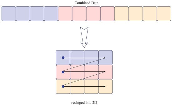
Figure 1.
Schematic diagram of the initial matrix generation.
- 4.
- Image remodeling
By filling the extension with the mirror, retaining the original data, and generating a three-channel RGB image through the gradient channel and nonlinear disturbance, we not only adapt the model’s input but also enhance its capacity for nonlinear feature capture.
(1) Mirror fill extension
The 224 × 78 matrix is expanded to a 224 × 224 matrix through mirror reflection, which involves mirroring the original sequence to the right of the original matrix until it fills the target 224 columns. This method preserves the original data, achieving a lossless dimensionality increase and avoiding the loss of nonlinear relationships that can occur with other methods, such as linear interpolation. Additionally, mirror reflection prevents edge artifacts, making it suitable for time series or spatial data. The expansion process is illustrated in Figure 2.
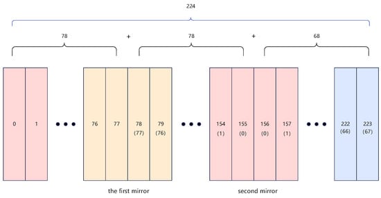
Figure 2.
Mirror reflection expansion.
(2) Three-channel generation
Channel 1 (Original Timing Channel): directly retain the data after mirror expansion of the original data as the basic channel, which can reflect the time-domain characteristics.
Channel 2 (longitudinal gradient channel-time difference): calculate the first-order difference of adjacent time points along the time axis (row direction), and apply MinMaxScaler to normalize the results to [−1, 1]
The mutation features in the time dimension are captured through this channel.
Channel 3 (horizontal gradient channel-feature difference): calculate the first-order difference of adjacent features along the feature axis (column direction) and apply MinMaxScaler to normalize the results to [−1, 1]
The coupling relationship between features is captured through this channel to effectively identify nonlinear attacks across features.
(3) Optimize processing
Add random noise: the add_noise parameter allows random noise to be added enhance the model’s robustness to perturbations.
Parallel processing: use ThreadPoolExecutor to perform parallel batch image transformation (transform, transform_with_labels) to improve the processing speed.
This transformation method is advantageous due to its high calculation efficiency and good data fidelity. At the same time, it provides multi-perspective expression of traffic data through three channels: basic time domain features, dynamic evolution features and cross-dimensional correlation features; effectively captures a variety of complex nonlinear attack modes; and is highly compatible with the MobileNetV3 model.
The corresponding pseudocode is shown in Algorithm 1.
| Algorithm 1. Four stages of flow data to image | |
| import: | D // Original flow data |
| output: | image_matrices // The three-channel image set |
| 1 | ND= MinMaxScaler (feature_range= (−1, 1)).fit_transform (D) // Stage 1: Feature standardization |
| 2 | window_size = 224, stride = 112, windows = [] // Stage 2: Time window division |
| for i in range(0, len(ND), stride): | |
| if len(window= ND[i:i+window_size]) < window_size: | |
| window = mirror_padding (window, target_length=window_size) // Mirror padding | |
| windows.append(window) | |
| 3 | image_matrices = [] // Stage 3:Spatial mapping |
| for window in windows: | |
| matrix = reshape (window, (window_size, 78)) // Converts to a 224 by 78 matrix | |
| 4 | mirrored_matrix = mirror_padding(matrix, axis=1, target_length=224) // Stage 4: Image remodeling |
| Channel 1 = mirrored_matrix, channel2 = time_axis_diff (channel 1), channel3 = feature_axis_diff (channel 1) // Generates three channels | |
| Image = stack([channel1, channel2, channel3], axis=2) // Merge three channels | |
| If add_noise: // Add random noise | |
| image += random_noise(image.shape) | |
| image_matrices.append(image) | |
| 5 | return image_matrices |
Through the aforementioned approach, the original traffic data are effectively transformed into corresponding visual representations. Figure 3 illustrates typical image samples of various attack types extracted from the CICIDS-2018 dataset. By analyzing the detailed visual features in these images, the MobileNetV3 model can more accurately identify and differentiate different types of network attacks, playing a crucial role in practical security defenses.
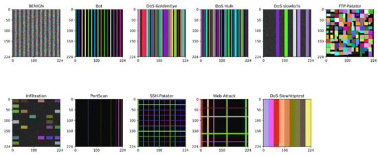
Figure 3.
Typical image samples of attack types in the CICIDS-2018 dataset.
3.2. Flow Anomaly Detection Framework
After the data transformation is completed, the preprocessed image is input into the improved IM-MobileNetV3 model for comprehensive training and verification.
3.2.1. Original MobileNetV3
MobileNetV3 [8] has excellent computing efficiency and high precision. Considering the strict real-time requirements of this scenario, the study adopts MobileNetV3-Small, a version of the model with a lighter weight, more compact structure, and lower computing delay, as the basic architecture, as shown in Figure 4.
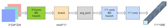
Figure 4.
MobileNetV3-Small architecture diagram.
In the model framework illustrated in Figure 4, the first part extracts spatial features using an initial standard convolution layer. This layer is a 3 × 3 convolution with a stride of 2 and 16 output channels, followed by a Hard–Swish activation function and batch normalization (BN). Efficient feature extraction and representation are achieved through a modular bottleneck block (bneck) design. Each bneck consists of multiple sub-components, including an expansion convolution, a depthwise separable convolution, a linear bottleneck, and an optional Squeeze-and-excitation module (SE module). In the final stage, GAP and two 1 × 1 point-wise convolutions are used to output the classification results. This structure design enables MobileNetV3 to be compact, low-computational, and high-precision. The specific parameter settings for each layer are detailed in Table 1.

Table 1.
MobileNetV3-Small’s parameters.
3.2.2. ECA Mechanism
The original MobileNetV3-Small utilized an SE [23] attention mechanism. Despite the numerous improvements that have been made to the model [24,25,26,27], such as enhancing its accuracy by capturing more complex channel dependencies or integrating spatial attention, these alterations often increase the model’s complexity and computational load. The Efficient Channel Attention Network (ECA-Net) [28] replaces the MLP module with a one-dimensional convolution (kernel size k), which avoids channel dimensionality reduction while significantly reducing computational costs. This addresses the limitations of SE blocks, ensuring a direct correspondence between channels and their weights, and effectively enabling cross-channel interaction [29,30]. The model diagram is shown in Figure 5.
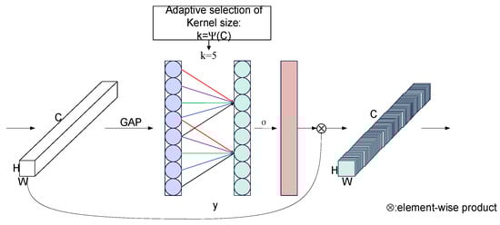
Figure 5.
ECA model diagram.
After performing GAP on the input feature map, a pooled feature vector y is obtained. This vector undergoes a one-dimensional convolution with a kernel size of k, where k is adaptively determined based on the channel dimension C. The convolution result is then normalized to the [0, 1] range using a Sigmoid function to obtain the channel weights. Multiplying these channel weights by the original input feature map completes the feature re-scaling.
The channel weight is calculated as follows:
Among them, is the Sigmoid function; C1D represents the fast 1D convolution; k is the kernel size and is the only unknown; and y is the aggregated feature vector obtained by GAP.
k is adaptively determined through the channel dimension C. A simple idea is to use to represent the channel dimension C, but the information of this linear function is very limited, and C is usually a power of 2. Therefore, it can be represented by the following nonlinear function:
Among them, are constants. When the channel dimension C is given, the kernel size k can be adaptively determined by the following formula:
Here, represents the closest odd number t. For all the experiments, we set and . This mapping ensures that the interaction range of low-dimensional features is smaller and that of high-dimensional features is larger.
3.2.3. Transfer Learning
As shown in Figure 6, transfer learning is a key research direction in the fields of machine learning and deep learning [31]. Its core principle involves leveraging the knowledge gained from the source task to enhance the performance of the target task [32]. In the transfer learning framework, there are typically differences between the source domain and the target domain, as well as between the source task and the target task, in terms of data distribution, feature space, or objectives. Knowledge transfer mechanisms facilitate cross-domain knowledge sharing and adaptation. Model fine-tuning is one of the commonly used techniques, in which pre-trained model parameters from the source task are used as initial weights, and the model is trained on the target task to make focused adjustments, enabling the model to quickly adapt to new task requirements. Studies have shown [33] that compared to training from scratch with randomly initialized parameters, the fine-tuning strategy can significantly accelerate model convergence and effectively improve the model’s accuracy and generalization ability.
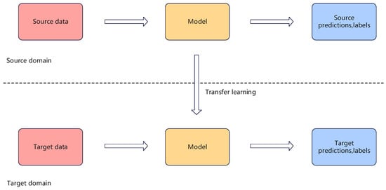
Figure 6.
Schematic diagram of transfer learning.
In this study, to enhance the model’s generalization ability in abnormal traffic detection, improve training efficiency, and achieve good training results, a two-stage transfer learning strategy is proposed, which involves freezing the pre-trained parameters of the ImageNet dataset (comprising approximately 1.2 million images) to retain the ability to extract general features, followed by unfreezing and fine-tuning all layer parameters. By utilizing the knowledge of general visual patterns embedded in large-scale image data, this transfer learning strategy provides effective initialization guidance for network traffic feature learning, thereby facilitating the transfer application of knowledge from different domains.
3.2.4. IM-MobileNetV3
In order to allow the model to more successfully adapt to the three-channel image of traffic data transformation and complete the abnormal detection task, the network structure of MobileNetV3 must be optimized and adjusted layer by layer. The specific parameters of the optimized lightweight real-time detection model IM-MobileNetV3 are shown in Table 2.
Table 2.
IM-MobileNetV3 parameters.
The main improvements are as follows:
- Attention Mechanism Improvement: the original SE attention module in the model has been replaced with an ECA module, which uses a one-dimensional convolutional structure instead of an MLP structure. This change avoids information loss during dimensionality reduction, maintains detection accuracy, and reduces computational complexity. Additionally, the ECA module is applied to all bneck structures and convolutional layers (except for 1 × 1 convolutions) throughout the network, enabling adaptive channel weight allocation. This enhances the model’s sensitivity to abnormal traffic by efficiently capturing network traffic features.
- Optimization of the initial convolution layer: the size of the convolution kernel in the first layer of the model is adjusted from 3 × 3 to 5 × 5 to increase the receptive field; meanwhile, the convolution stride is changed from 2 to 1, so as to better retain the detailed feature information at the bottom layer and ensure the fine-grained flow pattern is not lost too early.
- Bottleneck Layer Structure Design: to preserve more of the model’s early features, the stride of the first bneck block is set to 1, and the stride gradually increases in subsequent bneck blocks while controlling the magnitude of stride changes, achieving an ideal balance between feature map size and computational efficiency. Additionally, since the task has shifted from a thousand-category classification task in ImageNet to a binary anomaly detection task, adjustments are made accordingly. In terms of feature expansion, the initial part maintains the expansion size to ensure the extraction of basic features, while later stages moderately reduce the expansion size to mitigate overfitting risks. In terms of channel dimensions, the number of output channels is reduced to better suit the needs of the binary detection task. Compared to the original model, the total number of modules is reduced, but each module’s feature extraction capability is enhanced, leading to a decrease in overall model parameters and computational complexity, and improved performance in anomaly traffic detection tasks.
- Enhancing the tail structure: replace the 1 × 1 convolutional layer with a 3 × 3 convolutional layer to improve the feature extraction of local abnormal patterns. Implement a dual-channel pooling strategy using GAP and GMP to complementarily extract features, where GMP effectively captures the sudden peak characteristics of abnormal traffic. Introduce high-probability Dropout in the classification layer to mitigate overfitting caused by the scarcity of abnormal samples. Additionally, replace the Softmax activation function with the Sigmoid function to better fit the probability output for binary classification tasks.
- Dynamic Learning Rate Scheduling Strategy: during training, the ReduceLROnPlateau learning rate scheduling is employed. If the loss function on the validation set decreases, the learning rate remains constant. Conversely, if there is no improvement, the learning rate is linearly reduced through annealing until it reaches a certain threshold, after which it stops decreasing. This approach helps prevent overfitting and enables the model to escape local optima, thereby accelerating convergence and enhancing detection accuracy.
The corresponding pseudo code for IM-MobileNetV3 traffic anomaly detection is shown in Algorithm 2.
| Algorithm 2. Traffic anomaly detection process | |
| import: | image_matrices, D // The preprocessed image set and the original traffic data |
| output: | results // Anomaly detection results set |
| 1 | model = load_pretrained_IM_MobileNetV3() // Load the pre-trained IM-MobileNetV3 model |
| 2 | batch_size = 32, results = [] // Batch processing of images |
| for batch in range(0, len(image_matrices), batch_size): | |
| Batch images = image_matrices[batch: batch+batch_size] // Extract the current batch of images | |
| 3 | Logits = model.forward(batch_images) // The forward inference is used to obtain the predicted value |
| 4 | Probabilities = sigmoid (logits) // Sigmoid activates the output probability value// Stage 4: Image remodeling |
| 5 | For prob in probability: // Determine the result |
| if prob > 0.5: | |
| results.append (“exceptional traffic”) | |
| else: | |
| results.append (“Normal traffic”) | |
| 6 | return results |
Together, these improvements allows IM-MobileNetV3 to perform significantly better than MobileNetV3-Small in network traffic anomaly detection tasks, with a clear increase in accuracy, robustness, and reasoning efficiency.
4. Experiments and Results
4.1. Experimental Settings
In this experiment, Python 3.10 was used for programming and the following key libraries were utilized: TensorFlow 2.14.0, PyTorch 2.1.0, NumPy 1.24.3, Pandas 2.1.1, Scikit-learn 1.3.1, OpenCV 4.8.0, and Matplotlib 3.9. Specifically, TensorFlow and PyTorch provided core support for building and training neural network models; NumPy offered efficient numerical computation capabilities; Pandas handled data processing and analysis; Scikit-learn provided traditional machine learning algorithms; OpenCV managed image-related tasks; and Matplotlib was used for result visualization and chart generation. The experiment was conducted on the Ubuntu 22.04 LTS operating system using a NVIDIA RTX 4090 24 GB GPU (Nvidia Corporation, Santa Clara, CA, USA), an Intel Xeon E5-2680 v4 (Intel Corporation, Santa Clara, CA, USA) or AMD EPYC 7742 CPU, 64 GB DDR4 memory, and a 1 TB NVMe SSD (Advanced Micro Devices, Inc., Santa Clara, CA, USA). The GPU, along with CUDA 12.2 and cuDNN 8.9.4, provided parallel computing power, while the large-capacity memory ensured smooth model operation, and the high-speed SSD guaranteed that data were read and written efficiently. In the previous part of the experiment, the dataset adopted CIC-IDS2018, and the training set and validation set were divided in a 7:3 ratio. In the extended experiment, three independent datasets—Bot-IoT, ton_iot, and UNSW-NB15—were added. The comparison models include MobileNetV3-Small, traditional CNN, LSTM, and random forest.
4.2. Evaluation Indicators
In order to comprehensively evaluate the performance of the model, the following core indicators are adopted:
Accuracy: the proportion of the number of samples correctly classified to the total number of samples, as shown in Formula (14).
Precision: the precision rate predicted as a positive example (and actually also a positive example), as shown in Formula (15).
Recall: the proportion of samples that are actually positive and correctly predicted as positive, as shown in Formula (16).
F1 score: the harmonic mean of precision and recall, which provides a single indicator to balance the two, as shown in Formula (17).
The Area Under the ROC Curve (AUC) is the area under the receiver operating characteristic (ROC) curve, which measures the model’s overall ability to distinguish between classes at different classification thresholds. A higher AUC value indicates a better performance. The ROC curve has the true-positive rate (TPR, or Recall) on the y-axis and the false-positive rate (FPR) on the x-axis, as shown in Formula (18).
The abbreviation TP stands for true positive, where the model predicts and actually classifies an instance as positive. For example, if the model predicts and classifies an instance as positive, it is a true positive. FP stands for false positive, a situation in which the model predicts an instance as positive but it is actually negative. For example, if the model predicts and classifies an instance as positive, it is a false positive. FN stands for false negative, where the model predicts an instance as negative, but it is actually positive. For example, if the model predicts and classifies an instance as negative, it is a false negative. TN stands for true negative, where the model predicts and classifies an instance as negative, and it is indeed negative. For example, if the model predicts and classifies an instance as negative, it is a true negative.
The model parameter quantity is the total number of learnable parameters of the model, which reflects the complexity of the model.
Training time is the time required for the model to complete its training on the training set.
The inference time per sample is the average time required by the model to predict a single new sample, which is a key indicator of real-time performance.
The above indicators are calculated based on the confusion matrix (including TP, TN, FP, and FN).
4.3. Component-Level Analysis
To verify the effectiveness of each improved component in the IM-MobileNetV3 model, we designed a systematic ablation experiment, in which the improved parts of the model were decomposed into five key components for step-by-step verification:
Component A: Attention Mechanism Improvement.
Component B: Optimization of the initial convolution layer.
Component C: Bottleneck Layer Structure Design.
Component D: Enhancing the tail structure.
Component E: Dynamic Learning Rate Scheduling Strategy.
Figure 7 shows the performance changes that occur as a result of gradual addition of the above components starting from the original MobileNetV3-Small baseline model:
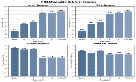
Figure 7.
The results of the IM-MobileNetV3 ablation experiment.
Accuracy, as the basic evaluation index, can visually demonstrate the prediction accuracy of the classifier on the overall dataset. The F1 score effectively compensates for the potential for misjudgment that arises when dealing with category-imbalanced data by integrating the precision and the recall. Furthermore, the number of parameters, as a direct quantitative representation of the model complexity, has a numerical magnitude directly related to the design scale of the model structure. The single-sample reasoning time objectively reflects the efficiency level of the model in real-time prediction. The experimental results provided the following insights:
- The introduction of Component A increased both the accuracy rate and the F1 score by four percentage points (84.5%→88.7%) while reducing the number of model parameters by 4.4% and lowering the inference time by 6.3%. This verifies that the ECA module effectively retains the feature information by avoiding the channel dimension reduction of SE; at the same time, its lightweight design improves the computational efficiency.
- Although Component B is associated with a slight increase in computational overhead, the accuracy rate further improves to 90.1%, and the F1 score further increases to 90.2%, demonstrating the importance of 5 × 5 convolution kernels increasing the receptive field and stride = 1 to preserve detailed features for traffic detection.
- Component C is responsible for the most significant performance improvement. The accuracy rate rises by 5.6 percentage points, the F1 score increases by 5.3 percentage points, while the number of parameters decreases by 31.2% and the inference time drops by 12.5%, indicating that the bottleneck layer structure optimized for traffic characteristics can extract key features more efficiently and accurately.
- Component D further increased the accuracy rate to 96.0% and the F1 score to 95.8% through the dual-pooling strategy and 3 × 3 convolution, verifying the effectiveness of the complementary feature extraction of GAP and GMP in capturing abnormal traffic patterns.
- Component E eventually increased the model accuracy rate and F1 score to 96.9%, indicating that the adaptive learning rate adjustment helps the model surpass the local optimum and achieve a better convergence effect.
The ablation experiments clearly demonstrated the ways in which each component contributes to the model performance. The optimization of the bottleneck layer and the ECA mechanism was the most crucial for performance improvement, while other components further refined the model’s capabilities. All the improvements, while enhancing the detection accuracy, maintained the lightweight characteristics (parameter count 1.20M) and real-time performance (inference time 2.8 ms) of the model, verifying the effectiveness of the design improvement of IM-MobileNetV3.
4.4. System-Level Verification
4.4.1. Classification Performance Comparison
In order to provide a more intuitive understanding of the performance of IM-MobileNetV3, MobileNetV3-Small, CNN, LSTM, and random forest in anomaly detection, Figure 8 shows the classification confusion matrix of these five models on CIC-IDS2018.
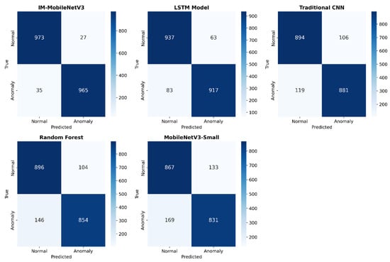
Figure 8.
Confusion matrix of five models.
As shown in Figure 8, IM-MobileNetV3 has the highest number of correct classifications and the lowest number of incorrect classifications. Moreover, both the TP and TN rates are higher than those of MobileNetV3-Small by more than 100 cases, clearly demonstrating its superior classification performance. To further quantify this comparison, the key classification metrics (accuracy, precision, recall, F1 score) for each model were summarized and visualized, as illustrated in Figure 9.
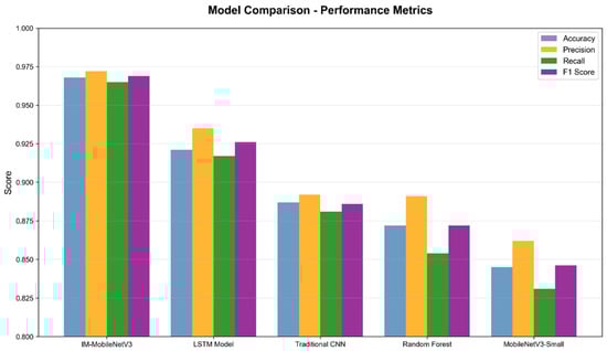
Figure 9.
Comparison of parameters of the five models.
As shown in Figure 9, IM-MobileNetV3 achieved the best results across all evaluation metrics (accuracy: 0.969, precision: 0.973, recall: 0.965, and F1 score: 0.969), significantly outperforming other models. The LSTM model followed closely, with all metrics exceeding 0.9. The CNN and random forest models performed similarly, with metrics above 0.85. The MobileNetV3-Small model had the weakest performance, highlighting the compatibility issues that arise when directly applying the original model structure to traffic detection tasks.
Figure 10 shows the ROC curves and corresponding AUC values of the five models on the CIC-IDS2018 dataset.
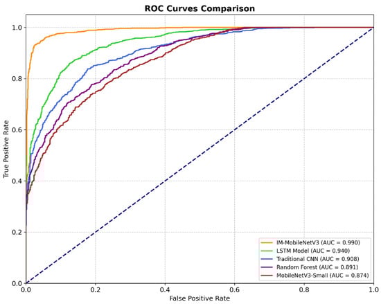
Figure 10.
ROC curves of five models.
The ROC curve and AUC value are crucial metrics for evaluating the performance of supervised learning in classification tasks. In the ROC space, a higher false-positive rate (FRP) and a true-positive rate (TPR) closer to 1 indicate better classification performance. The point (0,1) represents the ideal classification with the highest performance. As shown in Figure 10, the ROC curve of the IM-MobileNetV3 model is closest to the top-left corner, with an AUC value of 0.990, significantly outperforming other models. The LSTM and CNN models have AUC values of 0.940 and 0.908, respectively, followed by the random forest model, which has an AUC value of 0.891, also close to 0.9. Lastly, the MobileNetV3-Small model has an AUC value of 0.874. This indicates that IM-MobileNetV3 excels in distinguishing between normal and abnormal traffic.
Figure 11 shows the variation trend of accuracy and validation loss of five types of models in the training process.
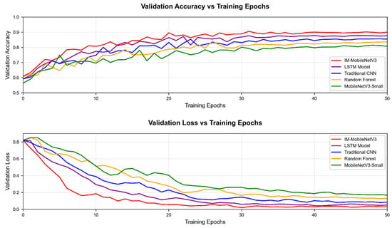
Figure 11.
Comparison of verification accuracy and verification loss of five models.
As shown in Figure 11, all models exhibit a trend towards convergence, with no significant overfitting (where the validation loss increases with training rounds) or underfitting (where the validation accuracy or loss stagnates at a poor level too early). Notably, IM-MobileNetV3 achieved the highest final accuracy and the lowest final loss on the validation set, indicating that it not only trains effectively but also demonstrates strong generalization capabilities.
The experimental results show that the improved IM-MobileNetV3 can successfully adapt to the abnormal traffic detection task, and achieves the best classification performance compared with the classical traditional model. It can achieve high classification accuracy while maintaining stability, and has good generalization ability.
4.4.2. Model Complexity and Efficiency Analysis
First, the number of model parameters is selected to determine whether the model has met the conditions required for real-time detection in the cloud environment and whether it has achieved a light weight and simple structure, as described in theory. The comparison results are shown in Figure 12.
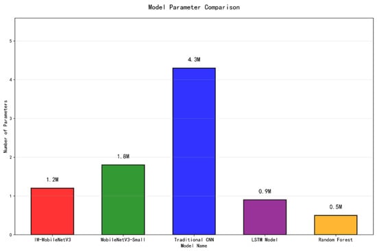
Figure 12.
Comparison of five types of model parameters.
Figure 12 compares the parameter sizes of five models. The optimized IM-MobileNetV3 model shows a 33% reduction in parameters compared to the original MobileNetV3-Small, which is significantly lower than the CNN model but slightly higher than the LSTM model and the random forest model. Although it ranks in the middle of the five models in terms of parameter size, IM-MobileNetV3 maintains its lightweight characteristics, with moderate structural complexity, meeting the requirements for real-time detection in cloud environments.
In order to further verify that the improved model is suitable for real-time detection, experiments on training time and reasoning time were conducted; the results are shown in Figure 13.
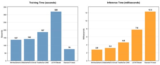
Figure 13.
Comparison of training time and reasoning time of five models.
Figure 13 compares the training time and inference time the models require for a single sample. IM-MobileNetV3 takes 137 s to train, which is only slightly higher than the random forest model with the fewest parameters and significantly lower than LSTM, CNN, and MobileNetV3-Small, indicating its high training efficiency. The inference time is the shortest among all models, at just 2.8 ms, far below random forest and LSTM, and less than one-quarter of the random forest’s time. Real-time detection involves processing new data using a pre-trained model, which places greater emphasis on the inference time for a single sample. The model only requires occasional updates, i.e., retraining, and the IM-MobileNetV3 model still demonstrates a significant advantage in real-time performance. These results indicate that the IM-MobileNetV3 model has low complexity and high efficiency.
4.4.3. Model Generalization Analysis
To verify the good generalization ability of IM-MobileNetV3, we conducted extended experiments on three independent datasets: Bot-IoT, ton_iot, and UNSW-NB15. These datasets address real cyberattack scenarios such as Internet of Things (IoT) device traffic and industrial Internet attacks. By comparing classification performance based on these datasets, we were able to effectively verify the generalization ability of the model. The key indicators are shown in Figure 14.
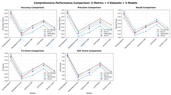
Figure 14.
A comparison chart of classification performance of five types of models on multiple datasets.
The extended experiments show that under all datasets, IM-MobileNetV3 achieves the best accuracy, precision, recall rate, F1 score, and AUC value, and has good classification accuracy, showing excellent generalization in both IoT traffic and real attack scenarios. Its method of converting four-stage data into images and the optimized network architecture can effectively adapt to the distribution differences of different types of traffic. This provides experimental support for the model’s deployment in multiple scenarios, such as cloud environments and edge computing nodes.
Comprehensive analysis shows that IM-MobileNetV3 can maintain its lightweight model structure (with a moderate number of parameters and a small absolute value), while achieving the highest detection accuracy (with the best classification indicators) and the fastest inference speed (2.8 ms). The model’s outstanding performance on the validation set and other data (Figure 10 and Figure 13) provides further evidence of its good generalization performance. Although its training time is slightly higher than that of random forest, its extremely low inference delay makes it more promising in real-time abnormal traffic detection scenarios in cloud environments that require millisecond-level responses.
5. Conclusions
This study aims to tackle the dual challenges of classification accuracy and real-time performance in abnormal traffic detection in the cloud environment using an improved lightweight real-time detection model: IM-MobileNetV3. The model’s lightweight, deep learning-based design was achieved through targeted optimization of the original MobileNetV3-Small architecture. The ECA mechanism was adopted to avoid the channel dimension reduction calculation of the SE module, and redundant channels were compressed to improve the structure of the bottleneck layer, etc. The number of model parameters is 33% lower than that of the original lightweight model MobileNetV3-Small, and it has only 1.2 million parameters. Meanwhile, in multiple datasets, the IM-MobileNetV3 model outperforms the other four models in terms of accuracy, precision, recall, F1 score, and AUC value, exhibiting good classification accuracy. Finally, the model can achieve a single-sample inference speed of 2.8 ms to meet the requirements of real-time response. Theoretically, it is better equipped to address the difficulties associated with balancing high detection accuracy and processing efficiency of complex traffic in the cloud environment. In future work, we will build a cloud-native testing platform to verify and optimize the deployment effect of the model in the real cloud environment.
Author Contributions
Conceptualization, Y.M. and W.F.; methodology, Y.M.; software, Y.M.; validation, Y.M., W.F., Y.Z. and J.C.; formal analysis, Y.Z.; investigation, J.C.; resources, W.F.; data curation, J.C.; writing—original draft preparation, Y.M.; writing—review and editing, Y.M., W.F., Y.Z. and J.C.; visualization, Y.Z.; supervision, J.C.; project administration, W.F.; funding acquisition, W.F. All authors have read and agreed to the published version of the manuscript.
Funding
This research was funded by National Natural Science Foundation of China (Grant No. 62276273) Research on Key Technologies for Multi Cloud Storage Data Security Based on Zero Trust Architecture.
Data Availability Statement
The original data presented in the study are openly available at Github at https://github.com/Afaf2003/Intrusion-Detection-System.
Conflicts of Interest
The authors declare no conflict of interest.
Abbreviations
The following abbreviations are used in this manuscript:
| ECA | Efficient Channel Attention. |
| SE | Squeeze-and-excitation networks. |
| DDoS | Distributed Denial of Service. |
| SVM | Support Vector Machine. |
| LSTM | Long Short-Term Memory. |
| CNN | Convolutional Neural Network. |
| MLP | Multilayer Perceptron. |
| GAP | Global average pooling. |
| GMP | Global maximum pooling. |
| DPCA | Dynamic Principal Component Analysis. |
| HMM | Hidden Markov Models. |
| TCP | Transmission Control Protocol. |
| DNS | Domain Name System. |
| ICMP | Internet Control Message Protocol. |
| NAS | Neural Architecture Search. |
| BN | Batch normalization. |
| TP | True positives. |
| FP | False positives. |
| FN | False negatives. |
| TN | True negatives. |
| IoT | Internet of Things. |
References
- Huawei Technologies Co., Ltd. Analysis of the Current Situation and Trends of Global DDoS Attacks in 2023. Available online: https://e.huawei.com/cn/material/networking/security/333e0bdd9694437e80aac4b436781fe3 (accessed on 20 February 2025).
- Yoachimik, O.; Pacheco, J. DDoS Report. Available online: https://blog.cloudflare.com/zh-cn/tag/ddos-reports/ (accessed on 20 February 2025).
- Cortes, C.; Vapnik, V. Support-vector networks. Mach. Learn. 1995, 20, 273–297. [Google Scholar] [CrossRef]
- Breiman, L. Random forests. Mach. Learn. 2001, 45, 5–32. [Google Scholar] [CrossRef]
- He, K.; Zhang, X.; Ren, S.; Sun, J. Deep residual learning for image recognition. In Proceedings of the IEEE Conference on Computer Vision and Pattern Recognition, Las Vegas, NE, USA, 26 June–1 July 2016. [Google Scholar]
- Hochreiter, S.; Schmidhuber, J. Long short-term memory. Neural Comput. 1997, 9, 1735–1780. [Google Scholar] [CrossRef] [PubMed]
- Lecun, Y.; Bottou, L.; Bengio, Y.; Haffner, P. Gradient-based learning applied to document recognition. Proc. IEEE 1998, 86, 2278–2324. [Google Scholar] [CrossRef]
- Howard, A.; Sandler, M.; Chu, G.; Chen, L.C.; Chen, B.; Tan, M.; Wang, W.; Zhu, Y.; Pang, R.; Vasudevan, V.; et al. Searching for MobileNetV3. In Proceedings of the 2019 IEEE/CVF International Conference on Computer Vision (ICCV), Seoul, Republic of Korea, 27 October–2 November 2019. [Google Scholar]
- Alajlan, A.M.; Almasri, M.M. Malicious behavior detection in cloud using self-optimized dynamic kernel convolutional neural network. Trans. Emerg. Telecommun. Technol. 2022, 33, e4449. [Google Scholar] [CrossRef]
- Huang, D.; Shi, X.; Zhang, W.A. False Data Injection Attack Detection for Industrial Control Systems Based on Both Time- and Frequency-Domain Analysis of Sensor Data. IEEE Internet Things J. 2021, 8, 585–595. [Google Scholar] [CrossRef]
- Ramprasath, J.; Ramakrishnan, S.; Tharani, V.; Sushmitha, R.; Arunima, D. Cloud service anomaly traffic detection using random forest. In Advances in Data and Information Sciences: Proceedings of ICDIS 2022; Springer: Berlin/Heidelberg, Germany, 2022; pp. 269–279. [Google Scholar]
- Bamasag, O.; Alsaeedi, A.; Munshi, A.; Alghazzawi, D.; Alshehri, S.; Jamjoom, A. Real-time DDoS flood attack monitoring and detection (RT-AMD) model for cloud computing. PeerJ Comput. Sci. 2022, 7, e814. [Google Scholar] [CrossRef]
- Girish, L.; Rao, S.K.N. Anomaly detection in cloud environment using artificial intelligence techniques. Computing 2023, 105, 675–688. [Google Scholar] [CrossRef]
- Sujatha, M.P.; Kumar, S.N. Anomaly Detection of Industrial Control Systems Based on Transfer Learning. Int. J. Health Sci. 2022, 6, 5782–5792. [Google Scholar] [CrossRef]
- Lin, K.; Xu, X.; Xiao, F. MFFusion: A Multi-level Features Fusion Model for Malicious Traffic Detection based on Deep Learning. Comput. Netw. 2022, 202, 108658. [Google Scholar] [CrossRef]
- Liu, H.; Han, F.; Zhang, Y. Malicious traffic detection for cloud-edge-end networks: A deep learning approach. Comput. Commun. 2024, 215, 150–156. [Google Scholar] [CrossRef]
- Hao, W.; Yang, T.; Yang, Q. Hybrid Statistical-Machine Learning for Real-Time Anomaly Detection in Industrial Cyber–Physical Systems. IEEE Trans. Autom. Sci. Eng. 2023, 20, 32–46. [Google Scholar] [CrossRef]
- Lv, X.; Han, D.; Li, D.; Xiao, L.; Chang, C.-C. Network abnormal traffic detection method based on fusion of chord similarity and multiple loss encoder. EURASIP J. Wirel. Commun. Netw. 2022, 2022, 105. [Google Scholar] [CrossRef]
- Yin, X.; Li, W.; Li, Z.; Yi, L. Recognition of grape leaf diseases using MobileNetV3 and deep transfer learning. Int. J. Agric. Biol. Eng. 2022, 15, 184–194. [Google Scholar] [CrossRef]
- Cao, Z.; Li, J.; Fang, L.; Li, Z.; Yang, H.; Dong, G. Research on efficient classification algorithm for coal and gangue based on improved MobilenetV3-small. Int. J. Coal Prep. Util. 2025, 45, 437–462. [Google Scholar] [CrossRef]
- Tian, X.; Shi, L.; Luo, Y.; Zhang, X. Garbage Classification Algorithm Based on Improved MobileNetV3. IEEE Access 2024, 12, 44799–44807. [Google Scholar] [CrossRef]
- Farrukh, Y.A.; Wali, S.; Khan, I.; Bastian, N.D. SeNet-I: An approach for detecting network intrusions through serialized network traffic images. Eng. Appl. Artif. Intell. 2023, 126, 107169. [Google Scholar] [CrossRef]
- Hu, J.; Shen, L.; Sun, G. Squeeze-and-excitation networks. In Proceedings of the IEEE Conference on Computer Vision and Pattern Recognition, Salt Lake City, UT, USA, 18–22 June 2018. [Google Scholar]
- Jin, X.; Xie, Y.; Wei, X.-S.; Zhao, B.-R.; Chen, Z.-M.; Tan, X. Delving deep into spatial pooling for squeeze-and-excitation networks. Pattern Recognit. 2022, 121, 108159. [Google Scholar] [CrossRef]
- Wang, J.; Luan, Z.; Yu, Z.; Ren, J.; Gao, J.; Yuan, K.; Xu, H. Superpixel segmentation with squeeze-and-excitation networks. Signal Image Video Process. 2022, 16, 1161–1168. [Google Scholar] [CrossRef]
- Mkindu, H.; Wu, L.; Zhao, Y. Lung nodule detection of CT images based on combining 3D-CNN and squeeze-and-excitation networks. Multimed. Tools Appl. 2023, 82, 25747–25760. [Google Scholar] [CrossRef]
- Zhang, G.; Choi, D.; Jung, J. Reconstruction of arterial blood pressure waveforms based on squeeze-and-excitation network models using electrocardiography and photoplethysmography signals. Knowl. Based Syst. 2024, 295, 111798. [Google Scholar] [CrossRef]
- Wang, Q.; Wu, B.; Zhu, P.; Li, P.; Zuo, W.; Hu, Q. ECA-Net: Efficient Channel Attention for Deep Convolutional Neural Networks. In Proceedings of the 2020 IEEE/CVF Conference on Computer Vision and Pattern Recognition (CVPR), Virtual, 14–19 June 2020. [Google Scholar]
- Wei, X.; Wang, Z. TCN-attention-HAR: Human activity recognition based on attention mechanism time convolutional network. Sci. Rep. 2024, 14, 7414. [Google Scholar] [CrossRef] [PubMed]
- Zhang, Y.; Zhan, Q.; Ma, Z. EfficientNet-ECA: A lightweight network based on efficient channel attention for class-imbalanced welding defects classification. Adv. Eng. Inform. 2024, 62, 102737. [Google Scholar] [CrossRef]
- Hosna, A.; Merry, E.; Gyalmo, J.; Alom, Z.; Aung, Z.; Azim, M.A. Transfer learning: A friendly introduction. J. Big Data 2022, 9, 102. [Google Scholar] [CrossRef]
- Zhao, Z.; Alzubaidi, L.; Zhang, J.; Duan, Y.; Gu, Y. A comparison review of transfer learning and self-supervised learning: Definitions, applications, advantages and limitations. Expert Syst. Appl. 2024, 242, 122807. [Google Scholar] [CrossRef]
- Yao, S.; Kang, Q.; Zhou, M.; Rawa, M.J.; Abusorrah, A. A survey of transfer learning for machinery diagnostics and prognostics. Artif. Intell. Rev. 2023, 56, 2871–2922. [Google Scholar] [CrossRef]
Disclaimer/Publisher’s Note: The statements, opinions and data contained in all publications are solely those of the individual author(s) and contributor(s) and not of MDPI and/or the editor(s). MDPI and/or the editor(s) disclaim responsibility for any injury to people or property resulting from any ideas, methods, instructions or products referred to in the content. |
© 2025 by the authors. Licensee MDPI, Basel, Switzerland. This article is an open access article distributed under the terms and conditions of the Creative Commons Attribution (CC BY) license (https://creativecommons.org/licenses/by/4.0/).