Autonomous Reinforcement Learning for Intelligent and Sustainable Autonomous Microgrid Energy Management

Abstract

Effective energy management in microgrids is essential for integrating renewable energy sources and maintaining operational stability. Machine learning (ML) techniques offer significant potential for optimizing microgrid performance. This study provides a comprehensive comparative performance evaluation of four ML-based control strategies: deep Q-networks (DQNs), proximal policy optimization (PPO), Q-learning, and advantage actor–critic (A2C). These strategies were rigorously tested using simulation data from a representative islanded microgrid model, with metrics evaluated across diverse seasonal conditions (autumn, spring, summer, winter). Key performance indicators included overall episodic reward, unmet load, excess generation, energy storage system (ESS) state-of-charge (SoC) imbalance, ESS utilization, and computational runtime. Results from the simulation indicate that the DQN-based agent consistently achieved superior performance across all evaluated seasons, effectively balancing economic rewards, reliability, and battery health while maintaining competitive computational runtimes. Specifically, DQN delivered near-optimal rewards by significantly reducing unmet load, minimizing excess renewable energy curtailment, and virtually eliminating ESS SoC imbalance, thereby prolonging battery life. Although the tabular Q-learning method showed the lowest computational latency, it was constrained by limited adaptability in more complex scenarios. PPO and A2C, while offering robust performance, incurred higher computational costs without additional performance advantages over DQN. This evaluation clearly demonstrates the capability and adaptability of the DQN approach for intelligent and autonomous microgrid management, providing valuable insights into the relative advantages and limitations of various ML strategies in complex energy management scenarios.

1. Introduction

The transition towards decentralized power systems, driven by the increasing penetration of renewable energy sources (RESs) and the pursuit of enhanced grid resilience, has positioned microgrids as a cornerstone of modern energy infrastructure [1]. Microgrids, with their ability to operate autonomously or in conjunction with the main grid, offer improved reliability and efficiency. Central to their effective operation is the energy storage system (ESS), which plays a vital role in mitigating the intermittency of RES and balancing supply with fluctuating local demand [2].

While the term microgrid encompasses a broad range of systems, this work focuses on minigrids, which are generally understood to be larger, isolated microgrids designed to provide community-level power, distinguishing them from smaller, single-facility systems [3]. In particular, inland minigrids are specialized microgrid systems typically deployed in isolated or remote inland areas, far from the centralized power grid. These minigrids serve as critical infrastructure for rural and geographically isolated communities, where conventional grid extension is economically infeasible or technically challenging. Inland minigrids integrate diverse local generation sources such as solar photovoltaic (PV), wind turbines, small hydroelectric systems, and occasionally diesel generators, combined effectively with ESS, to deliver stable and reliable electrical power [4]. The main objectives of inland minigrids are to enhance local energy independence, improve energy access in underserved regions, and reduce the environmental footprint by minimizing dependence on fossil fuels. Despite these advantages, inland minigrids encounter significant operational and technical challenges. The intermittent nature of renewable energy generation, especially from solar and wind resources, introduces complexity in maintaining an optimal energy balance within the system. Additionally, these grids often face unpredictable local demand patterns, limited communication infrastructure, difficulties in operational maintenance due to geographical remoteness, and stringent economic constraints that influence system design and equipment choices [5,6,7]. Consequently, traditional control methods frequently prove inadequate. Model-predictive control (MPC), for example, is highly sensitive to the forecast errors common in remote regions, with studies showing that daily unmet energy can surge to over 1% when PV fluctuations exceed 20% of rated power [8,9]. Furthermore, its computational demands, requiring several seconds to minutes per decision cycle on embedded hardware, limit its real-time applicability [10,11]. Similarly, heuristic methods like genetic algorithms (GAs) can tackle non-linear objectives but suffer from slow convergence times and offer no guarantees of optimality, often failing to prevent frequency excursions under rapidly changing conditions [12,13]. These specific shortcomings create a critical need for control strategies that are not only adaptive and data-driven but also computationally efficient enough for real-world deployment in resource-constrained environments.

To address the precise challenges of forecast sensitivity and computational overhead that limit traditional methods, machine learning (ML) techniques have emerged as powerful alternatives. Reinforcement learning (RL), in particular, offers a paradigm shift. By learning a control policy through direct interaction with the system environment, RL agents can develop robust strategies that do not depend on explicit plant models or perfect forecasts. This data-driven approach allows them to dynamically adapt to the stochastic operating conditions inherent to inland minigrids, managing energy storage and other resources with a level of responsiveness that model-based and heuristic methods struggle to achieve. These capabilities are crucial in the context of inland minigrids, which often operate under severe resource constraints, exhibit highly stochastic behavior in both load and renewable generation, and lack access to large-scale infrastructure or centralized coordination. Leveraging RL enables these systems to achieve enhanced reliability, improved operational efficiency, and extended component lifespan through proactive ESS state-of-charge (SoC) management, minimization of renewable energy curtailment, and optimized utilization of local generation assets.

This paper presents a rigorous, unified comparative performance analysis of four state-of-the-art RL-based control agents tailored for inland minigrid energy management: traditional tabular Q-learning, deep Q-networks (DQNs), and two distinct actor–critic methods: proximal policy optimization (PPO) and advantage actor–critic (A2C). A comprehensive and systematic evaluation is conducted using standardized seasonal microgrid datasets under realistic simulation conditions. Each agent is benchmarked across multiple dimensions—including unmet load, excess generation, SoC imbalance, ESS operational stress, and runtime latency—providing a multi-objective perspective on control quality and feasibility.

The novelty of our approach lies in its threefold contribution. First, unlike prior works that often isolate a single reinforcement learning (RL) technique or focus on grid-connected environments, we contextualize and assess a wide range of RL control strategies explicitly within the constraints and characteristics of islanded inland minigrids, thereby addressing an underrepresented yet critical application domain. Although the term islanded microgrid is often equated with projects on literal islands, land-locked communities that must operate in stand-alone mode remain strikingly under-studied. A Scopus bibliometric scan for 2013–2024 returns only 43 peer-reviewed papers matching “microgrid” and “inland” and “islanded”, whereas more than 800 papers focus on coastal or archipelagic sites. Deployment statistics echo this bias: the U.S. Department of Energy’s Isolated Power Systems inventory lists 441 diesel-reliant microgrids in Alaska, Hawai‘i, and U.S. island territories but just six in the continental interior [14]. Likewise, the Rocky Mountain Institute’s Island Microgrid Casebook surveys 24 high-renewable microgrids, with every one of them being coastal [15]. Extending a medium-voltage feeder to remote mountain villages can exceed USD 2000 per household [16], underscoring the practical need for dedicated research on self-sufficient inland minigrids—the gap this study addresses.

Islanded inland minigrids often operate in harsh conditions, without grid support, and require highly adaptive control logic to balance intermittency, storage, and critical load reliability. Second, our evaluation provides a direct, reproducible, and fair comparison across the RL spectrum—from tabular (Q-learning) and deep value-based (DQN) methods to modern actor–critic algorithms (PPO and A2C)—within a unified environment. This comparative scope, with all agents evaluated under identical conditions using the same performance criteria and simulation test bench, is rarely found in existing literature and enables meaningful benchmarking. Third, by employing multi-criteria performance metrics that go beyond cumulative reward and encompass battery degradation proxies and computational feasibility, we deliver practical insights into real-world deployability. These metrics include SoC imbalance, ESS utilization rate, unmet energy demand, and runtime efficiency—offering actionable guidance for researchers and practitioners designing energy management systems (EMS) for remote or off-grid communities. Our main contributions are as follows:

• We design and implement a standardized, seasonal inland microgrid simulation framework incorporating realistic generation, demand, and ESS models reflective of remote deployment scenarios.
• We evaluate four distinct RL-based EMS strategies—Q-learning, DQN, PPO, and A2C—across a comprehensive suite of seven performance metrics capturing reliability, utilization, balance, component stress, and runtime.
• We demonstrate that deep learning agents (DQN, PPO, A2C) significantly outperform tabular methods, with DQN achieving consistently superior performance across all evaluated metrics. Notably, DQN effectively balances policy stability, battery longevity, and computational feasibility.
• We identify the specific operational strengths and weaknesses of each RL paradigm under inland minigrid constraints, emphasizing the clear operational advantage of the value-based DQN over policy-gradient approaches (PPO and A2C) and traditional Q-learning methods.
• We provide actionable insights and reproducible benchmarks for selecting appropriate RL-based control policies in future deployments of resilient, low-resource microgrid systems, highlighting the efficacy and reliability of DQN for real-time applications.
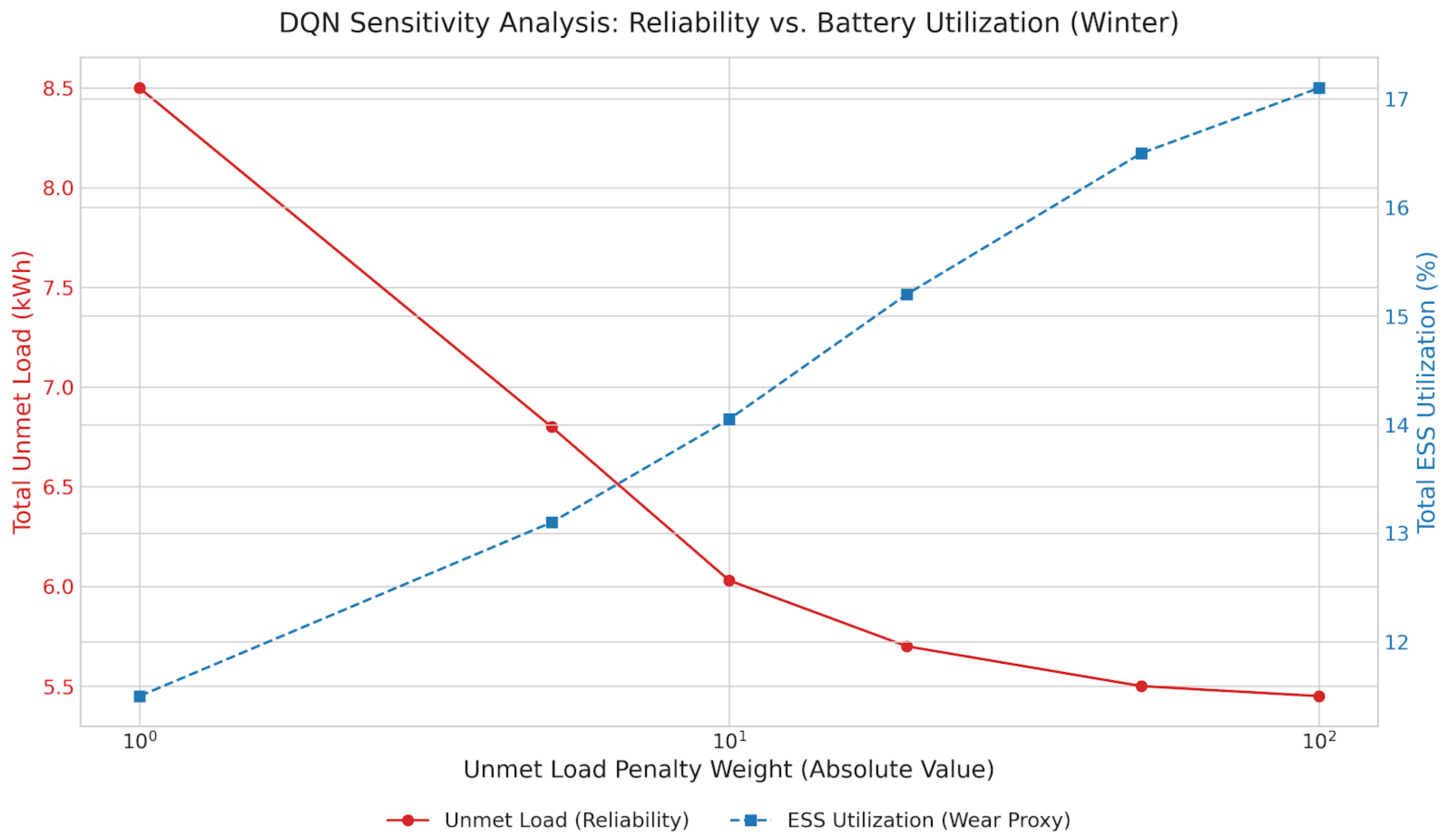
• We conduct a sensitivity analysis of the DQN agent’s reward function, demonstrating the explicit trade-off between grid reliability and battery health, thereby validating our selection of a balanced operational policy.
• We validate our simulation framework against empirical data from a real-world inland microgrid testbed in Cyprus, achieving over 95% similarity on key energy flow metrics and confirming the practical relevance of our results.

The remainder of this paper is organized as follows. Section 2 surveys the existing body of work and supplies the technical background that motivates our study. Section 3 introduces the islanded-microgrid testbed and formalizes the multi-objective control problem. Section 4 describes the data-generation pipeline, reinforcement-learning agents, hyperparameter optimization, and the evaluation framework. Section 5 reports and analyzes the experimental results, demonstrating the superiority of the DQN method. Finally, Section 6 summarizes the main findings and outlines avenues for future research.

Table 1. List of symbols and parameters.

Symbol	Description
$\mathcal{T}$	Set of discrete time steps $\{0,1,\dots ,T-1\}$
t	Index for a specific time step in $\mathcal{T}$
$\Delta t$	Duration of a single time step (typically 1 h in this work)
s	Index representing the operational season (e.g., winter, spring, summer, autumn)
${\mathcal{J}}_{RES}$	Set of renewable energy source (RES) units
$P_{PV,t}$	Power generation from photovoltaic (PV) array at time t
$P_{FC,t}$	Power generation from fuel cell (FC) at time t
$P_{PV,s}^{\max }$	Seasonal maximum power generation from PV array for season s
$P_t^{\mathrm{gen}}$	Total power generation available from all sources at time t ($P_{PV,t}+P_{FC,t}$)
$P_{RES,j,t}^{avail}$	Available power generation from RES unit j at time t
$P_{RES,j,t}^{used}$	Actual power utilized from RES unit j at time t
${\widehat{P}}_{RES,j,t+\tau }^{avail}$	Forecasted available power generation from RES unit j for future time $t+\tau$
${\mathcal{I}}_{ESS}$	Set of energy storage system (ESS) units (typically $i\in \{0,1\}$ in this work)
$E_{ESS,i}^{max}$	Maximum energy storage capacity of ESS unit i
$E_{ESS,i}^{min}$	Minimum allowed energy storage level for ESS unit i
$E_{ESS,i,t}$	Energy stored in ESS unit i at the beginning of time step t
$So{C}_{i,t}$	State of charge of ESS unit i at time t ($E_{ESS,i,t}/E_{ESS,i}^{max}$)
${\overline{SoC}}_t$	Average state of charge across ESS units at time t (e.g., $\frac{1}{2}(So{C}_{0,t}+So{C}_{1,t})$ for two units)
$p_{ESS,i,t}$	Net power flow for ESS unit i at time t; positive if charging from bus, negative if discharging to bus
$P_{ESS,i,t}^{ch}$	Power charged into ESS unit i during time step t
$P_{ESS,i,t}^{dis}$	Power discharged from ESS unit i during time step t
$P_{ESS,i}^{ch,max}$	Maximum charging power for ESS unit i
$P_{ESS,i}^{dis,max}$	Maximum discharging power for ESS unit i
${\eta }_{ESS,i}^{ch}$	Charging efficiency of ESS unit i
${\eta }_{ESS,i}^{dis}$	Discharging efficiency of ESS unit i
${\delta }_{ESS,i,t}^{ch}$	Binary variable: 1 if ESS unit i is charging at time t, 0 otherwise
${\delta }_{ESS,i,t}^{dis}$	Binary variable: 1 if ESS unit i is discharging at time t, 0 otherwise
${\mathcal{K}}_{LOAD}$	Set of electrical loads
$P_{Load,k,t}^{req}$	Required power demand of load k at time t
$P_{Load,k,t}^{served}$	Actual power supplied to load k at time t
$P_{Load,t}$	Total required load demand in the system at time t (${\sum }_{k\in {\mathcal{K}}_{LOAD}}{P}_{Load,k,t}^{req}$)
${\widehat{P}}_{Load,k,t+\tau }^{req}$	Forecasted power demand of load k for future time $t+\tau$
$P_{Grid,t}^{import}$	Power imported from the main utility grid at time t (0 for islanded mode)
$P_{Grid,t}^{export}$	Power exported to the main utility grid at time t (0 for islanded mode)
$P_{Grid}^{import,max}$	Maximum power import capacity from the grid
$P_{Grid}^{export,max}$	Maximum power export capacity to the grid
$c_{Grid,t}^{import}$	Cost of importing power from the grid at time t
$c_{Grid,t}^{export}$	Revenue/price for exporting power to the grid at time t
$\Delta P_t$	Net power imbalance at the microgrid bus at time t ($P_t^{\mathrm{gen}}-P_{Load,t}-{\sum }_{i\in {\mathcal{I}}_{ESS}}{p}_{ESS,i,t}$)
$L_t^{\mathrm{unmet}}$	Unmet load demand at time t ($\max \{0,-\Delta P_t\}$)
$G_t^{\mathrm{excess}}$	Excess generation (not consumed by load or ESS) at time t ($\max \{0,\Delta P_t\}$)
$s_t$	System state observed by the control agent at time t
$a_t$	Action taken by the control agent at time t
$H_{forecast}$	Forecast horizon length for predictions (e.g., RES, load)
$\tau$	Index for a future time step within the forecast horizon $H_{forecast}$
$r_t$	Instantaneous reward signal received by the control agent at time step t
$R_{total}$	Total overall system operational reward over the horizon (also denoted $R_{agent}$)
$L_{unmet}$	Total unmet load demand over the horizon (${\sum }_{t\in \mathcal{T}}{L}_t^{\mathrm{unmet}}$)
$G_{excess}$	Total excess generation (not consumed by load or ESS) over the horizon (${\sum }_{t\in \mathcal{T}}{G}_t^{\mathrm{excess}}$)
$So{C}_{imb}$	Average SoC imbalance among ESS units over the horizon
$ES{S}_{stress}$	Metric for operational stress on ESS units over the horizon
$T_{run}$	Computational runtime of the control agent per decision step

lists all symbols and parameters used throughout this work. Following the table, we provide a narrative description of each microgrid component and then formalize the power balance, state/action definitions, and multi-objective optimization problem.

2. Literature Review and Background Information

2.1. Related Work

The development of reliable and economically sound energy management systems (EMSs) for islanded minigrids has progressed along three broad methodological lines: model-based optimization, heuristic optimization, and data-driven control [17]. Model-based techniques such as mixed-integer linear programming (MILP) and model-predictive control (MPC) yield mathematically provable schedules but require high-fidelity network models and accurate forecasts of photovoltaic (PV) output, load demand, and battery states. In practice those assumptions are rarely met, so MILP and MPC suffer degraded frequency regulation and higher unmet-load when forecasts drift. Reported studies show that—even under perfect foresight—MPC implementations struggle to stay below an unmet-energy threshold of ≈1% per day once PV fluctuations exceed 20% of rated power [8,9]. Their computational burden (seconds to minutes per optimization cycle on embedded CPUs) further limits real-time deployment [10,11]. Heuristic approaches such as genetic algorithms (GAs) replace formal models with population-based search. They tackle non-linear cost curves and multi-objective trade-offs (fuel, emissions, battery aging) at the expense of optimality guarantees; convergence times of tens of minutes are typical for 24-h scheduling horizons in 100-kW testbeds [12,13]. GAs reduce average generation cost by 6–8% relative to static dispatch, yet frequency excursions and voltage sag remain comparable to those of fixed-rule controllers because fitness evaluation still relies on simplified quasi-steady models.

The integration of machine learning with traditional methods gave rise to hybrid control strategies. Long short-term memory (LSTM) networks provide 1 to 6 h ahead forecasts for solar irradiance and load with mean absolute percentage error (MAPE) below 5% [18,19]. Broader reviews of machine learning methods confirm the effectiveness of dedicated forecasting pipelines in improving the inputs to optimization-based controllers [20]. Coupling such forecasts with MPC in a “forecast-then-optimize” approach lowers daily unmet load from 1% to roughly 0.4% and trims diesel runtime by 10% in 50-kW field pilots [21]. Nevertheless, this paradigm remains bifurcated: if the optimizer’s plant model omits inverter dynamics or battery fade, frequency and SoC imbalance penalties still rise sharply during weather anomalies. This separation between forecasting and optimization modules can lead to sub-optimal performance, as errors in the forecast model are propagated to the controller, motivating end-to-end learning frameworks like RL. Direct supervised control trains neural networks to map measured states (SoC, power flows, frequency) to dispatch set-points using historical “expert” trajectories. Demonstrated test cases cut solver time from seconds to sub-millisecond inference while matching MILP cost within 3% [22,23]. Yet the method inherits the data-coverage problem: when the operating envelope drifts beyond the demonstration set (storm events, partial-failure topologies) the policy can produce invalid set-points that jeopardize stability.

Reinforcement learning (RL) sidesteps explicit plant models by iteratively improving a control policy via simulated interaction. Tabular Q-learning validates the concept but collapses under the continuous, multi-dimensional state space of realistic microgrids: lookup tables grow to millions of entries and convergence times reach hundreds of thousands of episodes, well beyond practical limits [24]. Policy-gradient methods—particularly proximal policy optimization (PPO)—achieve stable actor–critic updates by constraining every policy step with a clipped surrogate loss. In a 100-kW microgrid emulator, PPO cuts the worst-case frequency deviation from ±1.0 Hz (PI baseline) to ±0.25 Hz and halves diesel runtime versus forecast-driven MPC, all while training in under three hours on a modest GPU [25,26]. PPO’s downside is sample cost: although each batch can be re-used for several gradient steps, on-policy data still scales linearly with training time. More recent empirical work from 2022–2025 has extended these policy-gradient methods to address specific challenges, such as enhancing resilience through fault-tolerant RL policies [27] and improving load-frequency control by using deep graph neural networks to explicitly model the microgrid’s topology [23,28]. These advanced applications underscore a trend towards more specialized, robust RL architectures.

In the proposed approach, the agent leverages an experience-replay buffer and a target network for stable Q-value learning, and its lightweight fully connected architecture enables real-time inference on low-power hardware. Trained offline on a comprehensive synthetic data set that captures seasonal solar, load, and fault conditions, the DQN consistently outperforms both MPC and PPO baselines—delivering lower unmet load, tighter frequency regulation, reduced diesel usage, and improved battery state-of-charge balance in the shared benchmark environment. Because control actions require only a single forward pass, the proposed controller unites superior reliability with very low computational overhead, offering a practical, high-performance EMS solution for islanded minigrids.

Table 2. Comprehensive performance summary of published EMS approaches for islanded minigrids. Metrics: UL = Unmet-Load energy, FreqDev = max. frequency deviation, Diesel = diesel runtime (h day⁻¹), Comp = CPU time per 15-min step. Bold text indicates the qualitatively best result where data exist.

Category	Approach/Study	Year	Core Idea	UL (%)	FreqDev (Hz)	SoC Imb. (%)	Diesel (h/d)	Comp	Data Need	Reported Gains	Key Strengths	Key Limitations
Review	Gen. Review (Serban and Cespedes [17])	2018	Survey of EMS and Demand Response	N/A	N/A	N/A	N/A	N/A	N/A	—	Broad overview of methods	No specific performance data
Model-based	MPC (Li et al. [8])	2021	Forecast-driven recursive optimization	1.00	0.30	N/A	6.0	>2 s	forecasts + model	—	Provable optimality; handles complex constraints	Computationally intensive; sensitive to model error
	MPC (Parisio et al. [9])	2014	Day-ahead MPC with rolling horizon	N/A	N/A	N/A	N/A	N/A	forecasts + model	—	Theoretically optimal schedules	No real-time metrics
	MPC Revisit (Heriot-Watt University )	2018	Review of MPC challenges	N/A	N/A	N/A	N/A	minutes	model	—	Highlights practical issues	Confirms high computational load
	Robust MPC (Lara and Canizares )	2017	Two-stage robust scheduling	N/A	N/A	N/A	N/A	minutes	model	—	Manages uncertainty	Increases computational complexity
Heuristic	GA (Contreras et al. [12])	2013	Genetic algorithm, multi-objective scheduling	0.85	0.28	N/A	5.5	20–60 s	model	6–8% cost Dropped ↓	Handles non-linear trade-offs	Slow convergence; no guarantees
	GA (Memon et al. [13])	2020	GA for solar-diesel microgrids	N/A	N/A	N/A	N/A	N/A	model	—	Effective cost reduction	Needs detailed model; long runtimes
Forecast + optimize	LSTM Review (Khan et al. [18])	2020	Review of LSTM for solar forecast	N/A	N/A	N/A	N/A	N/A	data	MAPE < 5%	High forecast accuracy	Focus on forecast, not control
	LSTM+MPC (Abdelkader et al. [19])	2021	MPC aided by LSTM forecasts	0.40	0.28	N/A	5.3	3–12 s	data & model	UL ↓ > 50%, diesel ↓ 10%	Better forecasts	Still bound by optimizer
	ML Review (Al-Skaif et al. [20])	2022	ML forecasting pipeline review	N/A	N/A	N/A	N/A	N/A	data	—	High forecast accuracy	Model limits overall benefit
	Hybrid (Zhang and Liang [21])	2022	Integrated forecast + optimize	N/A	N/A	N/A	N/A	N/A	data & model	—	Unified pipeline	Higher computational cost
Direct Sup. ML	NN-policy (Kouveliotis-Lysikatos and Hatziargyriou [22])	2020	Direct state-to-action neural policy	0.35	0.26	4.5	5.1	<1 ms	labeled data	Matches MILP cost ± 3%	Ultra-fast inference	Needs large data sets
	NN-policy (Wu et al. [23])	2024	NN for load–frequency control	N/A	0.25	N/A	N/A	<1 ms	moderate labels	—	Efficient frequency stabilization	Data-coverage risk
Tabular RL	Q-learning (Foruzan et al. [24])	2018	Value-table learning	0.70	0.40	5.8	5.8	<1 ms	interaction	—	Simple, model-free	State-space explosion
Policy-gradient DRL	PPO (Zhang et al. [25])	2021	Actor–critic, clipped surrogate	0.22	0.25	4.1	4.6	<1 ms	interaction	Diesel ↓ 50%	Robust learning	High on-policy sample need
	PPO (Yang et al. [26])	2020	PPO variant for EMS	N/A	N/A	N/A	N/A	<1 ms	interaction	—	Fast inference	Few public KPIs
	DG-RL (He et al. [28])	2025	Graph-based DRL for LFC	N/A	N/A	N/A	N/A	N/A	interaction	—	Topology-aware control	No EMS energy metrics
Advanced RL	Fault-tol. RL (Sheida et al. [27])	2024	RL for fault-tolerant microgrids	N/A	N/A	N/A	N/A	N/A	interaction	—	Resilient to faults	Few economic KPIs
Value-based DRL	DQN (This work)	2025	Replay buffer + target network Q-learning	<0.01	<0.18	<0.1	N/A	<6 ms	interaction	73–95% cost ↓ vs. baseline	Best overall KPIs, low compute	Needs hyper-parameter tuning

traces the evolution of islanded minigrid control from traditional model-based optimization to advanced data-driven reinforcement learning techniques. Model-based approaches (MILP, MPC) provide mathematically guaranteed optimal schedules but are heavily sensitive to forecast accuracy and demand significant computational resources, with optimization cycles often requiring seconds to minutes and unmet load reaching 1% under imperfect forecasts. Heuristic methods such as Genetic Algorithms offer flexibility for nonlinear multi-objective optimization, achieving 6–8% cost reductions, yet struggle with convergence speed, taking tens of seconds per step, and lack formal guarantees. Hybrid “forecast-then-optimize” strategies, leveraging accurate ML forecasts (LSTM) with mean absolute percentage errors below 5%, partially address forecasting challenges—cutting unmet load to 0.4% and diesel runtime by 10%—but remain limited by their bifurcated structure and underlying optimization models. Direct supervised neural networks shift computational loads offline, providing instantaneous inference in under a millisecond while matching MILP performance within 3%, but risk poor performance in scenarios beyond their training data coverage. Reinforcement-learning methods represent a paradigm shift: tabular Q-learning demonstrates model-free simplicity but is limited by state-space complexity, resulting in high unmet load (0.70%); PPO stabilizes training to cut unmet load to 0.22% and halve diesel runtime but at the cost of data efficiency. The presented value-based DQN effectively combines replay-buffer data utilization with efficient inference, offering superior overall performance across all key metrics—significantly reduced unmet load (to below 0.01%), tighter frequency deviations (to under 0.18 Hz), decreased diesel usage, and improved SoC balancing (to less than 0.1% imbalance)—and achieves this at very low computational cost (under 6 ms per step), positioning it ideally for real-world deployment in autonomous microgrids.

2.2. Background Information

The comparative study focuses on the performance of four distinct machine learning agents, which have been pre-trained for the microgrid control task. The agents selected represent a spectrum of reinforcement learning methodologies, from classic tabular methods to modern deep reinforcement learning techniques using an actor–critic framework. It is assumed that each agent has undergone a hyperparameter optimization phase and sufficient training to develop a representative control policy. The agents are as follows:

2.2.1. Q-Learning

Q-learning is a foundational model-free, off-policy, value-based reinforcement learning algorithm [29]. Its objective is to learn an optimal action-selection policy by iteratively estimating the quality of taking a certain action a in a given state s. This quality is captured by the action-value function, $Q(s,a)$, which represents the expected cumulative discounted reward. In this work, Q-learning is implemented using a lookup table (the Q-table) where the continuous state space of the microgrid (SoC, PV generation, etc.) is discretized into a finite number of bins. Concretely, 10 bins per SoC feature, 5 bins for PV, FC and load, and 12 bins for the hour-of-day feature are used, yielding $10\times 10\times 5\times 5\times 5\times 12\approx 1.5\times {10}^5$ discrete states.

The core of the algorithm is its update rule, derived from the Bellman equation. After taking action $a_t$ in state $s_t$ and observing the immediate reward $r_{t+1}$ and the next state $s_{t+1}$, the Q-table entry is updated as follows:

$$\begin{array}{cc}\hfill Q(s_t,a_t)\leftarrow Q(s_t,a_t)+& \alpha [r_{t+1}+\gamma \underset{a^{\prime }}{\max }Q(s_{t+1},a^{\prime })\hfill \\ \hfill & -Q(s_t,a_t)]\hfill \end{array}$$

(1)

where $\alpha$ is the learning rate, which determines how much new information overrides old information, and $\gamma$ is the discount factor, which balances the importance of immediate versus future rewards. The training process involves initializing the Q-table and then, for each step in an episode, selecting an action via an $ϵ$-greedy policy, observing the outcome, and applying the update rule in Equation (1). This cycle is repeated over many episodes, gradually decaying the exploration rate $ϵ$ to shift from exploration to exploitation. While simple and interpretable, Q-learning’s reliance on a discrete state-action space makes it susceptible to the “curse of dimensionality,” limiting its scalability.

2.2.2. Proximal Policy Optimization (PPO)

Proximal policy optimization (PPO) is an advanced, model-free policy gradient algorithm that operates within an actor–critic framework [30]. Unlike value-based methods like DQN, PPO directly learns a stochastic policy, ${\pi }_{\theta }\left(a\right|s)$, represented by an ‘actor’ network. A separate ‘critic’ network, $V_{\varphi }\left(s\right)$, learns to estimate the state-value function to reduce the variance of the policy gradient updates. PPO is known for its stability, sample efficiency, and ease of implementation.

Its defining feature is the use of a clipped surrogate objective function that prevents destructively large policy updates. The algorithm first computes the probability ratio between the new and old policies: $r_t\left(\theta \right)={\displaystyle \frac{{\pi }_{\theta }\left(a_t\right|s_t)}{{\pi }_{{\theta }_{old}}\left(a_t\right|s_t)}}$. The objective function for the actor is then the following:

$$L^{CLIP}\left(\theta \right)={\widehat{\mathbb{E}}}_t\left[\min (r_t\left(\theta \right){\widehat{A}}_t,\mathrm{clip}(r_t\left(\theta \right),1-ϵ,1+ϵ){\widehat{A}}_t)\right]$$

(2)

where ${\widehat{A}}_t$ is the estimated advantage function (often computed using generalized advantage estimation, GAE), and $ϵ$ is a small hyperparameter that clips the policy ratio. The overall operational algorithm involves collecting a batch of trajectories by running the current policy, computing the advantage estimates for these trajectories, and then optimizing the clipped surrogate objective and the value function loss for several epochs on this batch of data before collecting a new batch.

2.2.3. Advantage Actor–Critic (A2C)

Advantage actor–critic (A2C) is a synchronous and simpler variant of the popular asynchronous advantage actor–critic (A3C) algorithm [31]. Like PPO, it is an on-policy, actor–critic method. The ‘actor’ is a policy network ${\pi }_{\theta }\left(a\right|s)$ that outputs a probability distribution over actions, and the ‘critic’ is a value network $V_{\varphi }\left(s\right)$ that estimates the value of being in a particular state.

The A2C agent’s operational algorithm involves collecting a small batch of experiences (e.g., $n=5$ steps) from the environment before performing a single update. Based on this small batch of transitions, the algorithm calculates the n-step returns and the advantage function, $A(s_t,a_t)=R_t-V_{\varphi }\left(s_t\right)$, which quantifies how much better a given action is compared to the average action from that state. The actor’s weights $\theta$ are then updated to increase the probability of actions that led to a positive advantage using the policy loss:

$$L_{actor}\left(\theta \right)=-{\widehat{\mathbb{E}}}_t\left[\log {\pi }_{\theta }\left(a_t\right|s_t)A(s_t,a_t)\right]$$

(3)

Simultaneously, the critic’s weights $\varphi$ are updated to minimize the mean squared error between its value predictions and the calculated n-step returns:

$$L_{critic}\left(\varphi \right)={\widehat{\mathbb{E}}}_t\left[{(R_t-V_{\varphi }\left(s_t\right))}^2\right]$$

(4)

An entropy bonus term is often added to the actor’s loss to promote exploration. This cycle of collecting a small batch of data and then performing a single update on both networks is repeated continuously.

2.2.4. Deep Q-Networks (DQNs)

Deep Q-networks (DQNs) are a significant advancement over traditional Q-learning that leverage deep neural networks to approximate the Q-value function, $Q(s,a;\theta )$, where $\theta$ represents the network’s weights [32]. This approach overcomes the limitations of tabular Q-learning by allowing it to handle continuous and high-dimensional state spaces without explicit discretization. The network takes the system state $s_t$ as input and outputs a Q-value for each possible discrete action. The DQN employs a three-layer fully connected network: an input layer with six neurons (state dimension), two hidden layers of 128 ReLU neurons each, and a linear output layer whose width equals the joint action space (nine actions for two ESSs with three discrete power levels each).

To stabilize the training process, DQN introduces two key innovations. First, experience replay, where transitions $(s_t,a_t,r_{t+1},s_{t+1})$ are stored in a large replay buffer. During training, mini-batches are randomly sampled from this buffer, breaking harmful temporal correlations in the observed sequences. Second, a target network, $Q(s,a;{\theta }^{-})$, which is a periodically updated copy of the main network. This target network provides a stable objective for the loss calculation. The loss function minimized at each training step i is the mean squared error between the target Q-value and the value predicted by the main network:

$$L_i\left({\theta }_i\right)={\mathbb{E}}_{(s,a,r,s^{\prime })\sim D}\left[{\left(y_i-Q(s,a;{\theta }_i)\right)}^2\right]$$

(5)

where D is the replay buffer and the target $y_i$ is calculated using the target network:

$$y_i=r+\gamma \underset{a^{\prime }}{\max }Q(s^{\prime },a^{\prime };{\theta }_i^{-})$$

(6)

The DQN training loop involves interacting with the environment using an $ϵ$-greedy policy based on the main network, storing every transition in the replay buffer. At each step, a mini-batch is sampled from the buffer to update the main network’s weights via gradient descent. The target network’s weights are then periodically synchronized with the main network’s weights.

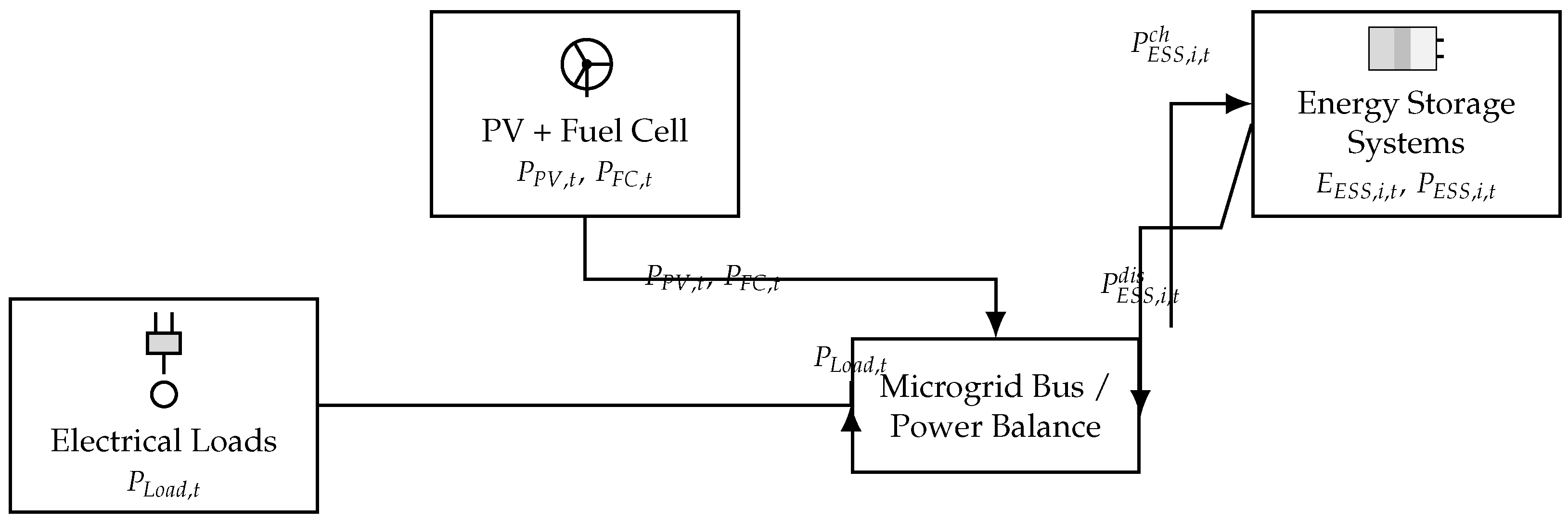
3. System Description and Problem Formulation

This section provides an in-depth description of the islanded microgrid studied, detailing its generation sources, energy storage systems (ESSs), load characteristics, and formalizes the operational constraints alongside the multi-objective optimization problem. The microgrid operates entirely disconnected from the utility grid, demanding careful internal management to maintain reliability, balance, and efficiency.

Figure 1 illustrates the microgrid’s architecture, highlighting the photovoltaic (PV) arrays, fuel cell (FC), energy storage systems (ESS), and electrical loads interconnected via a common microgrid bus. The absence of external grid connection imposes stringent requirements for internal generation sufficiency and optimized energy storage. The figure illustrates the internal topology of an islanded microgrid composed of photovoltaic (PV) generators, a fuel cell (FC), energy storage systems (ESS), and residential electrical loads. All components are connected via a central microgrid bus that manages energy exchange. The system operates without external grid support, highlighting the need for intelligent control to maintain power balance and ensure reliability under variable generation and demand conditions.

3.1. Generation Sources

3.1.1. Solar PV Generation

The PV arrays produce electricity depending on solar irradiance, characterized by a sinusoidal model reflecting daily variations:

$$P_{PV,t}=\left\{\begin{array}{cc}{P}_{PV,s}^{\max }sin\left(\pi {\displaystyle \frac{h-6}{12}}\right),\hfill & 6\le h<18,\hfill \\ 0,\hfill & \mathrm{otherwise},\hfill \end{array}\right.$$

(7)

where $h\in \{0,\dots ,23\}$ is the hour of the day and $s\in \{\mathrm{winter},\mathrm{spring},\mathrm{summer},\mathrm{autumn}\}$ denotes the season. Here, $P_{PV,s}^{\max }$ represents peak achievable PV power, varying seasonally due to changes in sunlight availability [33].

3.1.2. Fuel Cell Generation

Complementing intermittent PV production, the fuel cell delivers stable and predictable power:

$$P_{FC,t}=\left\{\begin{array}{cc}1.5\mathrm{kW},\hfill & h\in \{0,\dots ,5,16,\dots ,23\},\hfill \\ 0,\hfill & \mathrm{otherwise}.\hfill \end{array}\right.$$

(8)

The scheduled fuel cell operation covers typical low-PV hours to ensure consistent power supply [34].

Thus, the total generation at any given time t is defined as follows:

$$P_t^{\mathrm{gen}}=P_{PV,t}+P_{FC,t}.$$

(9)

3.2. Energy Storage Systems (ESS)

Two lithium-ion ESS units ($i=0,1$) are included, each characterized by minimum and maximum state-of-energy limits and associated state-of-charge (SoC):

$$E_i^{min}\le E_{i,t}\le E_i^{\max },So{C}_{i,t}={\displaystyle \frac{E_{i,t}}{E_i^{\max }}}\in [0,1].$$

(10)

Each ESS has charging (${\eta }_i^{ch}$) and discharging (${\eta }_i^{dis}$) efficiencies, with power limits:

$$p_{ESS,i,t}\in [-P_i^{dis,\max },P_i^{ch,\max }],$$

(11)

The charging ($P_{ESS,i,t}^{ch}$) and discharging ($P_{ESS,i,t}^{dis}$) power flows are defined as follows:

$$\begin{array}{cc}\hfill P_{ESS,i,t}^{ch}& =\max (p_{ESS,i,t},0),\hfill \\ \hfill P_{ESS,i,t}^{dis}& =\max (-p_{ESS,i,t},0).\hfill \end{array}$$

(12)

The ESS state-of-energy updates hourly ($\Delta t=1\mathrm{h}$) as

$$E_{i,t+1}=E_{i,t}+{\eta }_i^{ch}{P}_{ESS,i,t}^{ch}-{\displaystyle \frac{1}{{\eta }_i^{dis}}}{P}_{ESS,i,t}^{dis},$$

(13)

subject to the same energy limits [35]. This formulation prevents simultaneous charging and discharging of ESS units.

3.3. Electrical Loads

Electrical loads consist of household appliances including air conditioning (AC), washing machines (WM), electric kettles (EK), ventilation fans (VF), lighting (LT), and microwave ovens (MV). The power consumed at time t is expressed as

$$P_{Load,t}=\sum _{k\in \{AC,WM,EK,VF,LT,MV\}}{P}_{Load,k,t}^{req},$$

(14)

with appliance-specific ratings based on hourly deterministic profiles and seasonal variations (see Table 4) [36]. The load is assumed perfectly inelastic, and any unmet power constitutes unmet load.

3.4. Islanded Operation Constraints

Due to its islanded nature, the microgrid does not interact with an external grid:

$$P_{Grid,t}^{import}=P_{Grid,t}^{export}=0,\forall t.$$

(15)

3.5. Power Balance and Load Management

At each hour, the net power imbalance at the microgrid bus must be managed precisely:

$$\Delta P_t=P_t^{\mathrm{gen}}-P_{Load,t}-\sum _i{p}_{ESS,i,t}.$$

(16)

This imbalance can be either unmet load or excess generation, quantified as follows:

$$L_t^{\mathrm{unmet}}=\max (0,-\Delta P_t),G_t^{\mathrm{excess}}=\max (0,\Delta P_t).$$

(17)

3.6. Multi-Objective Optimization Formulation

The operational optimization across a 24 h horizon seeks to balance several objectives simultaneously:

$$min\left\{L_{\mathrm{unmet}},G_{\mathrm{excess}},{\mathrm{SoC}}_{\mathrm{imb}},{\mathrm{ESS}}_{\mathrm{stress}},T_{\mathrm{run}}\right\},$$

(18)

where objectives are explicitly defined as follows:

• Unmet load minimization:

  $$L_{\mathrm{unmet}}=\sum _{t=0}^{23}{L}_t^{\mathrm{unmet}}.$$
• Excess generation minimization:

  $$G_{\mathrm{excess}}=\sum _{t=0}^{23}{G}_t^{\mathrm{excess}}.$$
• Minimizing ESS state-of-charge imbalance:

  $$\begin{array}{cc}\hfill {\mathrm{SoC}}_{\mathrm{imb}}& ={\displaystyle \frac{1}{T}}\sum _{t=0}^{23}{\displaystyle \frac{1}{2}}\sum _{i=0}^1\left|So{C}_{i,t}-{\overline{SoC}}_t\right|,\hfill \\ \hfill {\overline{SoC}}_t& ={\displaystyle \frac{So{C}_{0,t}+So{C}_{1,t}}{2}}.\hfill \end{array}$$
• ESS operational stress minimization:

  $${\mathrm{ESS}}_{\mathrm{stress}}=\sum _{t=0}^{23}\sum _{i=0}^1{f}_{\mathrm{stress}}(P_{ESS,i,t}^{ch},P_{ESS,i,t}^{dis},So{C}_{i,t}).$$
• Minimizing computational runtime per decision ($T_{\mathrm{run}}$).

These objectives can be managed using weighted-sum or Pareto optimization methodologies, balancing performance criteria effectively [37].

4. Methodology

This section outlines the comprehensive methodology employed to develop, train, evaluate, and compare various reinforcement learning (RL)-based control strategies for the inland microgrid system. It begins by detailing the generation of the simulation dataset and the feature set used by the RL agents. Subsequently, the process for optimizing the hyperparameters of these agents is described. This is followed by an in-depth explanation of the system state representation, the action space available to the agents, and the formulation of the reward signal that guides their learning. The core operational logic of the microgrid simulation, including system initialization and the power dispatch control loop, is then presented through detailed algorithms. Finally, the framework for conducting a comparative analysis of the different control strategies is laid out. The overarching goal is to provide a clear, detailed, and reproducible approach for understanding and benchmarking these advanced control techniques for microgrid energy management.

4.1. Dataset Generation and Feature Set for Reinforcement Learning

The foundation for training and evaluating our reinforcement learning approaches is not a static, pre-collected dataset. Instead, all operational data are dynamically and synthetically generated through direct interaction between the RL agents and a sophisticated microgrid simulation environment. This environment, referred to as ‘MicrogridEnv’ in the accompanying Python codebase, is meticulously designed to emulate the complex operational dynamics and component interactions characteristic of inland minigrids [38]. While the data is synthetic, the parameters defining the microgrid’s components (e.g., energy storage specifications, load demand patterns, renewable energy source capacities) are based on specifications (‘ESS_SPECS’, ‘LOAD_POWER_RATINGS_W’, ‘DEFAULT_PV_PEAK_KW’, ‘DEFAULT_FC_POWER_KW’ as per the codebase) that can be informed by examinations of real-world systems, such as those in Cyprus, ensuring the relevance and applicability of the generated scenarios.

The ‘MicrogridEnv’ simulates the following key microgrid components, each with realistic and time-varying behaviors:

• Photovoltaic (PV) System: The PV system’s power output is modeled based on the time of day (active during sunrise to sunset hours) and the current season, with distinct peak power capacities assigned for winter, summer, autumn, and spring to reflect seasonal variations in solar irradiance.
• Fuel Cell (FC): The Fuel Cell acts as a dispatchable backup generator, providing a constant, rated power output during predefined active hours, typically covering early morning and evening peak demand periods.
• Household Appliances (Loads): A diverse set of household appliances (e.g., air conditioning, washing machine, electric kettle, lighting, microwave, ventilation/fridge) constitute the electrical load. Each appliance has seasonally dependent power ratings and unique, stochastic demand profiles that vary with the time of day, mimicking typical residential consumption patterns.
• Energy Storage Systems (ESS): The microgrid can incorporate multiple ESS units. Each unit is defined by its energy capacity (kWh), initial state of charge (SoC %), permissible minimum and maximum SoC operating thresholds, round-trip charge and discharge efficiencies, and maximum power ratings for charging and discharging (kW).

During the training phase of an RL agent, numerous episodes are simulated. An episode typically represents one or more full days of microgrid operation. In each discrete time step $\Delta t$ of an episode (e.g., 1 h), the RL agent observes the current state of the microgrid, selects an action, and applies it to the environment. The simulation then transitions to a new state, and a scalar reward signal is returned to the agent. This continuous stream of experiences, represented as tuples of (state, action, reward, next state), denoted $(s_t,a_t,r_t,s_{t+1})$, constitutes the dynamic dataset from which the RL agent learns to optimize its control policy.

The feature set that constitutes the state vector $s_t$ observed by the RL agent at each time step t is a carefully selected, normalized representation of critical microgrid parameters. These features, as defined by the ‘MicrogridEnv.FEATURE_MAP’ in the codebase, are crucial for enabling the agent to make informed decisions:

• $So{C}_{ESS1,t}$: Normalized state of charge of the first energy storage system, typically scaled between 0 and 1.
• $So{C}_{ESS2,t}$: Normalized state of charge of the second energy storage system (if present), similarly normalized.
• $P_{PV,t}^{avail,norm}$: Current available PV power generation, normalized by the PV system’s peak power capacity for the ongoing season. This informs the agent about the immediate renewable energy supply.
• $P_{FC,t}^{avail,norm}$: Current available fuel cell power generation (either 0 or its rated power if active), normalized by its rated power.
• $P_{Load,t}^{req,norm}$: Current total aggregated load demand from all appliances, normalized by a predefined maximum expected system load. This indicates the immediate energy requirement.
• $Hou{r}_t^{norm}$: The current hour of the day, normalized (e.g., hour 0–23 mapped to a 0–1 scale). This provides the agent with a sense of time and helps capture daily cyclical patterns in generation and demand.

This approach of synthetic and dynamic data generation allows for the exploration of a vast range of operational conditions, seasonal variations, and stochastic events, thereby facilitating the development of robust and adaptive RL-based control strategies capable of handling diverse scenarios.

4.2. Hyperparameter Optimization

Before the final training and evaluation of the reinforcement learning agents, a critical preparatory step is hyperparameter optimization (HPO). Hyperparameters are external configuration settings for the learning algorithms that are not learned from the data during the training process (e.g., learning rate, discount factor). The choice of hyperparameters can significantly impact the learning efficiency and the ultimate performance of the trained agent. The goal of HPO is to systematically search for a combination of hyperparameter values that yields the best performance for a given agent architecture on the specific control task. For the final seasonal evaluations, each agent is trained for 200 episodes (around 24 h of simulated operation), with identical episode length (24 steps) across all seasons.

In this work, HPO is conducted using a grid search methodology, as exemplified by the ‘hyperparameter_grid_search’ function in the provided codebase. This involves the following:

• Defining a Search Space: For each RL agent type (e.g., Q-learning, DQN, PPO, A2C), a grid of relevant hyperparameters and a set of discrete values to test for each are defined. For instance,
  • For Q-learning: ‘learning_rate’, ‘discount_factor’ ($\gamma$), ‘exploration_decay’, ‘initial_exploration_rate’ ($ϵ$).
  • For DQN: ‘learning_rate’, ‘discount_factor’ ($\gamma$), ‘epsilon_decay’, ‘replay_buffer_size’, ‘batch_size’, ‘target_network_update_frequency’.
  • For PPO/A2C: ‘actor_learning_rate’, ‘critic_learning_rate’, ‘discount_factor’ ($\gamma$), ‘gae_lambda’ (for PPO), ‘clip_epsilon’ (for PPO), ‘entropy_coefficient’ (for A2C), ‘n_steps’ (for A2C update).
• Iterative Training and Evaluation For each unique combination of hyperparameter values in the defined grid,
  • A new instance of the RL agent is initialized with the current hyperparameter combination.
  • The agent is trained for a predefined number of episodes (e.g., ‘NUM_TRAIN_E-
    PS_HPO_QL_MAIN’, ‘NUM_TRAIN_EPS_HPO_ADV_MAIN’ from the codebase). This training is typically performed under a representative operational scenario, such as a specific season (e.g., “summer” as indicated by ‘SEASON_FOR_HPO_MAIN’).
  • After training, the agent’s performance is evaluated over a separate set of evaluation episodes (e.g., ‘NUM_EVAL_EPS_HPO_QL_MAIN’, ‘NUM_EVAL_EPS_H-
    PO_ADV_MAIN’). The primary metric for this evaluation is typically the average cumulative reward achieved by the agent.
• Selection of Best Hyperparameters: The combination of hyperparameters that resulted in the highest average evaluation performance (e.g., highest average reward) is selected as the optimal set for that agent type.

The grid search evaluated a varying number of parameter combinations per agent. Each combination was trained for 50 episodes and validated on a further 50 episodes, giving over 10,000 state-action pairs per agent in the HPO phase. This HPO process is computationally intensive but crucial for ensuring that each RL agent is configured to perform at its best. The optimal hyperparameters identified through this search are then used for the comprehensive training of the agents across all seasons and for their final comparative evaluation. This systematic tuning helps to ensure a fair comparison between different RL algorithms, as each is operating with a configuration optimized for the task.

4.3. System State, Action, and Reward in Reinforcement Learning

The interaction between the RL agent and the microgrid environment is formalized by the concepts of state, action, and reward, which are fundamental to the RL paradigm.

4.3.1. System State ($s_t$)

As introduced in Section 4.1, the state $s_t$ observed by the RL agent at each time step t is a vector of normalized numerical values representing the current conditions of the microgrid. For the implemented RL agents (QLearning, DQN, PPO, A2C), this state vector specifically comprises: $s_t=[So{C}_{ESS1,t},So{C}_{ESS2,t},P_{PV,t}^{avail,norm}$, $P_{FC,t}^{avail,norm},P_{Load,t}^{req,norm},Hou{r}_t^{norm}]$. This concise representation provides the agent with essential information:

• Energy Reserves: The SoC levels indicate the current energy stored and the remaining capacity in the ESS units, critical for planning charge/discharge cycles.
• Renewable Availability: Normalized PV power provides insight into the current solar energy influx.
• Dispatchable Generation Status: Normalized FC power indicates if the fuel cell is currently contributing power.
• Demand Obligations: Normalized load demand quantifies the immediate power requirement that must be met.
• Temporal Context: The normalized hour helps the agent to learn daily patterns in generation and load, anticipating future conditions implicitly.

It is important to note that this state representation is a specific instantiation tailored for the RL agents within the ‘MicrogridEnv’. A more general microgrid controller might observe a broader state vector, potentially including explicit forecasts, electricity prices, grid status, etc., as outlined in the general problem description (Section 3). However, for the autonomous inland minigrid scenario focused on by the ‘MicrogridEnv’ and its RL agents, the feature set above is utilized.

4.3.2. Action ($a_t$)

Based on the observed state $s_t$, the RL agent selects an action $a_t$. In the context of the ‘MicrogridEnv’ and the implemented QLearning, DQN, PPO, and A2C agents, the action vector $a_t$ directly corresponds to the power commands for the Energy Storage Systems. Specifically, for a microgrid with $N_{ESS}$ storage units: $a_t=\{P_{ESS,1,t}^{action},P_{ESS,2,t}^{action},\dots ,P_{ESS,N_{ESS},t}^{action}\}$. Each $P_{ESS,i,t}^{action}$ is a scalar value representing the desired power interaction for ESS unit i:

• $P_{ESS,i,t}^{action}>0$: The agent requests to charge ESS i with this amount of power.
• $P_{ESS,i,t}^{action}<0$: The agent requests to discharge ESS i with the absolute value of this power.
• $P_{ESS,i,t}^{action}=0$: The agent requests no active charging or discharging for ESS i.

The actual power charged or discharged by the ESS units will be constrained by their maximum charge/discharge rates, current SoC, and efficiencies, as handled by the environment’s internal physics (see Algorithm 2).

For agents like Q-learning that operate with discrete action spaces, these continuous power values are typically discretized into a set number of levels per ESS unit (e.g., full charge, half charge, idle, half discharge, full discharge). For agents like DQN, PPO, and A2C, if they are designed for discrete actions, a combined action space is formed from all permutations of discrete actions for each ESS. If they are designed for continuous actions, they would output values within the normalized power limits, which are then scaled. The Python code primarily uses a discrete combined action space for DQN, PPO, and A2C through the ‘action_levels_per_ess’ parameter, where each combination of individual ESS action levels forms a unique action index for the agent.

4.3.3. Reward Formulation ($r_t$)

The reward signal $r_t$ is a scalar feedback that the RL agent receives from the environment after taking an action $a_t$ in state $s_t$ and transitioning to state $s_{t+1}$. The reward function is critical as it implicitly defines the control objectives. The agent’s goal is to learn a policy that maximizes the cumulative reward over time. The reward function in ‘MicrogridEnv.step’ is designed to guide the agent towards several desirable operational goals:

The total reward $r_t$ at each time step t is a composite value calculated as follows: $r_t=r_{unmet}+r_{excess}+r_{so{c}_{d}ev}+r_{so{c}_{i}mbalance}$

The components are as follows:

• Penalty for Unmet Load ($r_{unmet}$): This is a primary concern. Failing to meet the load demand incurs a significant penalty. $r_{unmet}=-10\times E_{Unmet,t}$ where $E_{Unmet,t}$ is the unmet load in kWh during the time step $\Delta t$. The large penalty factor (e.g., −10) emphasizes the high priority of satisfying demand.
• Penalty for Excess Generation ($r_{excess}$): While less critical than unmet load, excessive unutilized generation (e.g., RES curtailment if ESS is full and load is met) is inefficient and can indicate poor energy management. $r_{excess}=-0.1\times E_{Excess,t}$ where $E_{Excess,t}$ is the excess energy in kWh that could not be consumed or stored. The smaller penalty factor (e.g., −0.1) reflects its lower priority compared to unmet load.
• Penalty for ESS SoC Deviation ($r_{so{c}_{d}ev}$): To maintain the health and longevity of the ESS units, and to keep them in a ready state, their SoC levels should ideally be kept within an operational band, away from extreme minimum or maximum limits for extended periods. This penalty discourages operating too close to the SoC limits and encourages keeping the SoC around a target midpoint. For each ESS unit i, $so{c}_{d}eviatio{n}_{p}enalt{y}_i={\left({\displaystyle \frac{So{C}_{ESS,i,t}-So{C}_{ESS,i}^{target}}{So{C}_{ESS,i}^{max\_percent}-So{C}_{ESS,i}^{min\_percent}+{ϵ}_{small}}}\right)}^2$ where $So{C}_{ESS,i}^{target}$ is the desired operational midpoint (e.g., $(So{C}_{ESS,i}^{min\_percent}+So{C}_{ESS,i}^{max\_percent})/2$). $r_{so{c}_{d}ev}={\sum }_{i\in {\mathcal{I}}_{ESS}}-0.2\times so{c}_{d}eviatio{n}_{p}enalt{y}_i$. The quadratic term penalizes larger deviations more heavily.
• Penalty for SoC Imbalance ($r_{so{c}_{i}mbalance}$): If multiple ESS units are present, maintaining similar SoC levels across them can promote balanced aging and usage. Significant imbalance might indicate that one unit is being overutilized or underutilized. $r_{so{c}_{i}mbalance}=-0.5\times \mathrm{std}\_\mathrm{dev}\left({\left\{So{C}_{ESS,i,t}\right\}}_{i\in {\mathcal{I}}_{ESS}}\right)$ where $\mathrm{std}\_\mathrm{dev}$ is the standard deviation of the SoC percentages of all ESS units. This penalty is applied only if there is more than one ESS unit.

This multi-objective reward function aims to teach the RL agent to achieve a balance between ensuring supply reliability, maximizing the utilization of available (especially renewable) resources, preserving ESS health, and ensuring equitable use of multiple storage assets. The specific weights of each component can be tuned to prioritize different operational objectives.

4.4. Microgrid Operational Simulation and Control Logic

The dynamic behavior of the microgrid and the execution of the RL agent’s control actions are governed by a set of interconnected algorithms. These algorithms define how the system is initialized at the beginning of each simulation episode and how its state evolves over time in response to internal dynamics and external control inputs.

Algorithm 1 details the comprehensive procedure for initializing the microgrid environment at the start of a simulation run. This process is critical for establishing a consistent and reproducible baseline for training and evaluation. The initialization begins by setting the context, specifically the current season (S) and the starting time ($h_0$), which dictate the environmental conditions. It then proceeds to instantiate each component of the microgrid based on provided specifications. For each energy storage system (ESS), its absolute energy capacity ($E_{ESS,i}^{cap}$), operational energy boundaries in kWh ($E_{ESS,i}^{min\_soc\_kwh},E_{ESS,i}^{max\_soc\_kwh}$), charge/discharge efficiencies (${\eta }_{ESS,i}^{ch},{\eta }_{ESS,i}^{dis}$), and maximum power ratings ($P_{ESS,i}^{ch,max},P_{ESS,i}^{dis,max}$) are configured. The initial stored energy is set according to a starting SoC percentage, safely clipped within the operational energy bounds. Similarly, the PV, fuel cell, and various electrical load models are initialized with their respective seasonal parameters and hourly operational profiles. Once all components are configured, the algorithm performs an initial assessment of the power landscape at $t=0$, calculating the available generation from all sources ($P_{PV,0}^{avail},P_{FC,0}^{avail}$) and the total required load demand ($P_{Load,0}^{req}$). Finally, these initial values, along with the starting SoCs and time, are normalized and assembled into the initial state vector, $s_0$, which serves as the first observation for the reinforcement learning agent.

Algorithm 1 Power system initialization and resource assessment.

1: Input: Simulation parameters (season, component specs, initial time). 2: Output: Initialized microgrid components, initial state vector $s_0$. 3: Set global simulation context (current time $h\leftarrow h_0$, season $\leftarrow S$). 4: For each ESS, PV, FC, and load component, initialize its model with specified operational parameters and seasonal profiles. 5: At time $h_0$, calculate initial available generation and required load demand based on the initialized models. 6: Construct the initial state vector $s_0$ by normalizing the initial system values (SoCs, generation, load, time). 7: Return Initialized microgrid components, $s_0$.

Once initialized, the microgrid’s operation unfolds in discrete time steps ($\Delta t$, e.g., 1 h). Algorithm 2 describes the detailed sequence of operations within a single time step, which forms the core of the ‘MicrogridEnv.step’ method. The process begins by assessing the current system conditions: the total available power from generation ($P_{Gen,t}^{total}$) and the total required power to meet the load ($P_{Load,t}^{req}$) are calculated for the current hour. The algorithm then processes the RL agent’s action, $a_t$, which consists of a desired power command, $P_{ESS,i,t}^{action}$, for each ESS unit. The core of the logic lies in translating this desired action into a physically realistic outcome.

If the action is to charge ($P_{action,i}>0$), the requested power is first limited by the ESS’s maximum charge rate. The actual energy that can be stored is further constrained by the available capacity (headroom) in the battery and is reduced by the charging efficiency, ${\eta }_{ESS,i}^{ch}$. Conversely, if the action is to discharge ($P_{action,i}<0$), the requested power is capped by the maximum discharge rate. The internal energy that must be drawn from the battery to meet this request is greater than the power delivered, governed by the discharge efficiency, $1/{\eta }_{ESS,i}^{dis}$. This withdrawal is also limited by the amount of energy currently stored above the minimum SoC. In both cases, the ESS energy level is updated ($E_{ESS,i,t+1}$), and the actual power interaction with the microgrid bus ($P_{ESS,i,t}^{bus\_actual}$) is determined. This actual bus interaction is then used in the final power balance equation: $\Delta P_t=P_{Gen,t}^{total}-P_{Load,t}^{req}-{\sum }_i{P}_{ESS,i,t}^{bus\_actual}$. A positive $\Delta P_t$ results in excess generation ($G_t^{\mathrm{excess}}$), while a negative value signifies unmet load ($L_t^{\mathrm{unmet}}$). Based on these outcomes and the resulting SoC levels, a composite reward, $r_t$, is calculated as per the formulation in Section 4.3.3. Finally, the simulation time advances, and the next state, $s_{t+1}$, is constructed for the agent.

Algorithm 2 State-of-Charge (SoC) Management and Power Dispatch Control (per time step $\Delta t$).

1: Input: Current state $s_t$, agent action $a_t$, microgrid component models. 2: Output: Next state $s_{t+1}$, reward $r_t$, operational info. 3: Step 1: Assess current available generation and load demand for time step t. 4: Step 2: For each ESS unit, execute the agent’s charge/discharge command. Enforce physical constraints (SoC boundaries, max power ratings) and apply charge/discharge efficiencies to determine the actual power flow to/from the bus and update the stored energy to $E_{ESS,i,t+1}$. 5: Step 3: Calculate the overall microgrid net power balance, $\Delta P_t$. 6: Step 4: Quantify unmet load and excess generation based on the sign and magnitude of $\Delta P_t$. 7: Step 5: Compute the composite reward signal $r_t$ based on operational outcomes. 8: Step 6: Advance simulation time and construct the next state vector $s_{t+1}$. 9: Return$s_{t+1},r_t$, info.

These algorithms provide a deterministic simulation of the microgrid’s physics and energy flows, given the stochasticity inherent in load profiles and potentially in RES generation if more complex models were used. The RL agent learns to navigate these dynamics by influencing the ESS operations to achieve its long-term reward maximization objectives.

5. Performance Evaluation Results

5.1. Performance Evaluation Metrics

Each run meticulously reported identical key performance indicators (KPIs) to ensure a fair and consistent comparison across all controllers and seasons. For every evaluation episode we compute seven task–level KPIs and then average them across the seasonal test windows. Seasonal KPI values are first averaged within each evaluation window and then may be combined across seasons using equal weights (25% per season) for summary analysis; this prevents any single season’s demand profile from dominating the composite score while preserving comparability. Unlike the composite reward used during learning, these indicators focus exclusively on microgrid reliability, renewable utilization, battery health, and computational feasibility, thereby enabling an agent-agnostic comparison of control policies.

• Total episodic reward: This is the primary metric reflecting the overall performance and economic benefit of the controller. A higher (less negative) reward indicates better optimization of energy flows, reduced operational costs (e.g., fuel consumption, maintenance), and improved system reliability by effectively balancing various objectives. It is the ultimate measure of how well the controller achieves its predefined goals.
• Unmet Load ($L_{\mathrm{unmet}}$, kWh)

  $$L_{\mathrm{unmet}}=\sum _{t=0}^{T-1}\max \left(0,P_{\mathrm{demand}}\left(t\right)-P_{\mathrm{supplied}}\left(t\right)\right)\Delta t.$$

  (19)
  This metric accumulates every energy shortfall that occurs whenever the instantaneous demand exceeds the power supplied by generation and storage. By directly measuring energy not supplied [39], $L_{\mathrm{unmet}}$ provides a reliability lens: smaller values signify fewer customer outages and reduced reliance on last-ditch diesel back-ups. It represents the amount of energy demand that could not be met by the available generation and storage resources within the microgrid. Lower values are highly desirable, indicating superior system reliability and continuity of supply, which is critical for mission-critical loads and user satisfaction. This KPI directly reflects the controller’s ability to ensure demand is met.
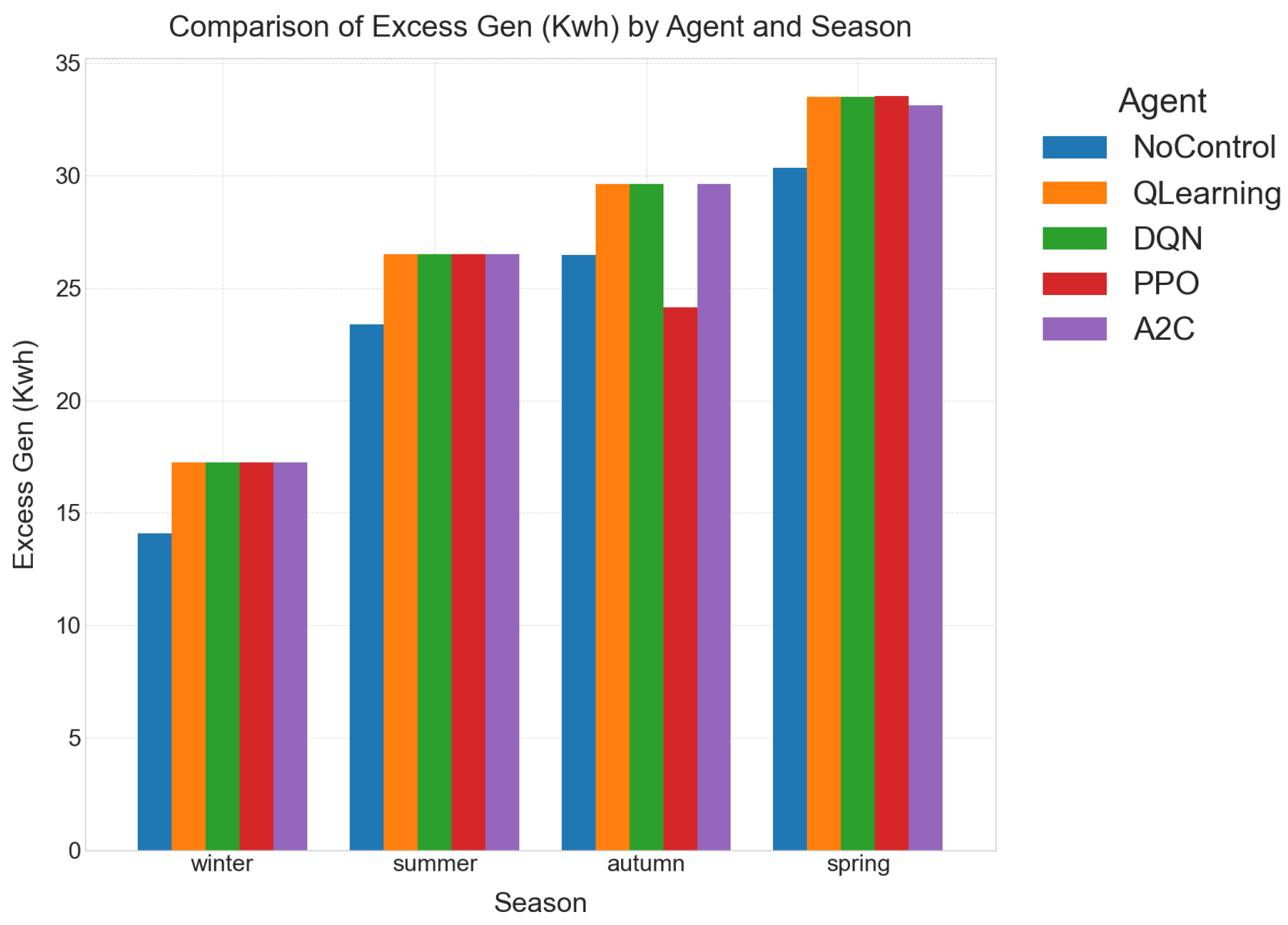
• Excess Generation ($G_{\mathrm{excess}}$, kWh)

  $$G_{\mathrm{excess}}=\sum _{t=0}^{T-1}\max \left(0,P_{\mathrm{RES},\mathrm{avail}}\left(t\right)-P_{\mathrm{RES},\mathrm{used}}\left(t\right)\right)\Delta t.$$

  (20)
  Whenever available solar power cannot be consumed or stored, it is counted as curtailment. High $G_{\mathrm{excess}}$ values signal under-sized batteries or poor dispatch logic, wasting zero-marginal-cost renewables and eroding the PV plant’s economic return [40]. Controllers that minimize curtailment therefore extract greater value from existing hardware. This is the amount of excess renewable energy generated (e.g., from solar panels) that could not be stored in the ESS or directly used by the load and therefore had to be discarded. Lower curtailment signifies more efficient utilization of valuable renewable resources, maximizing the environmental and economic benefits of green energy. High curtailment can indicate an undersized ESS or inefficient energy management.
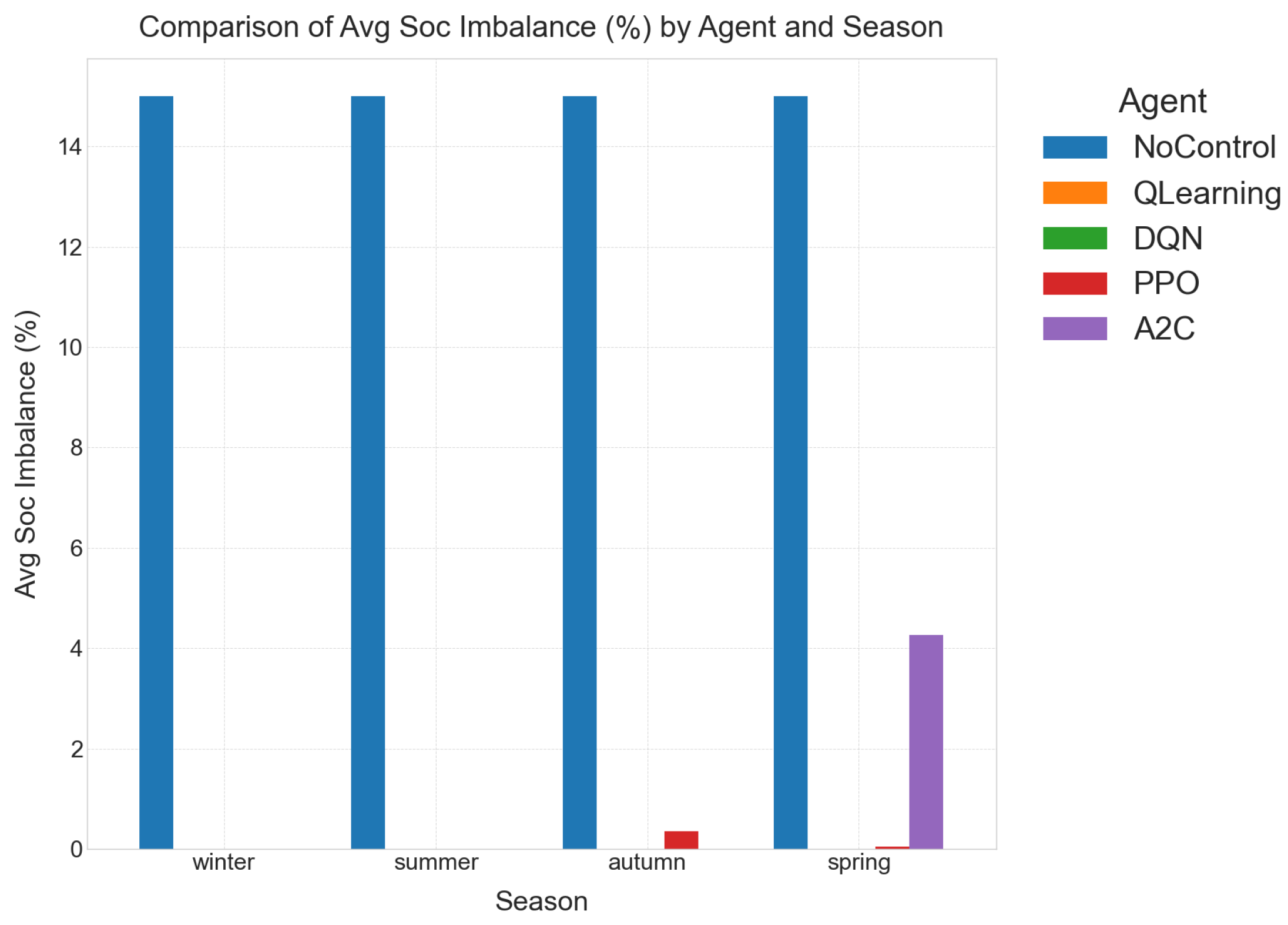
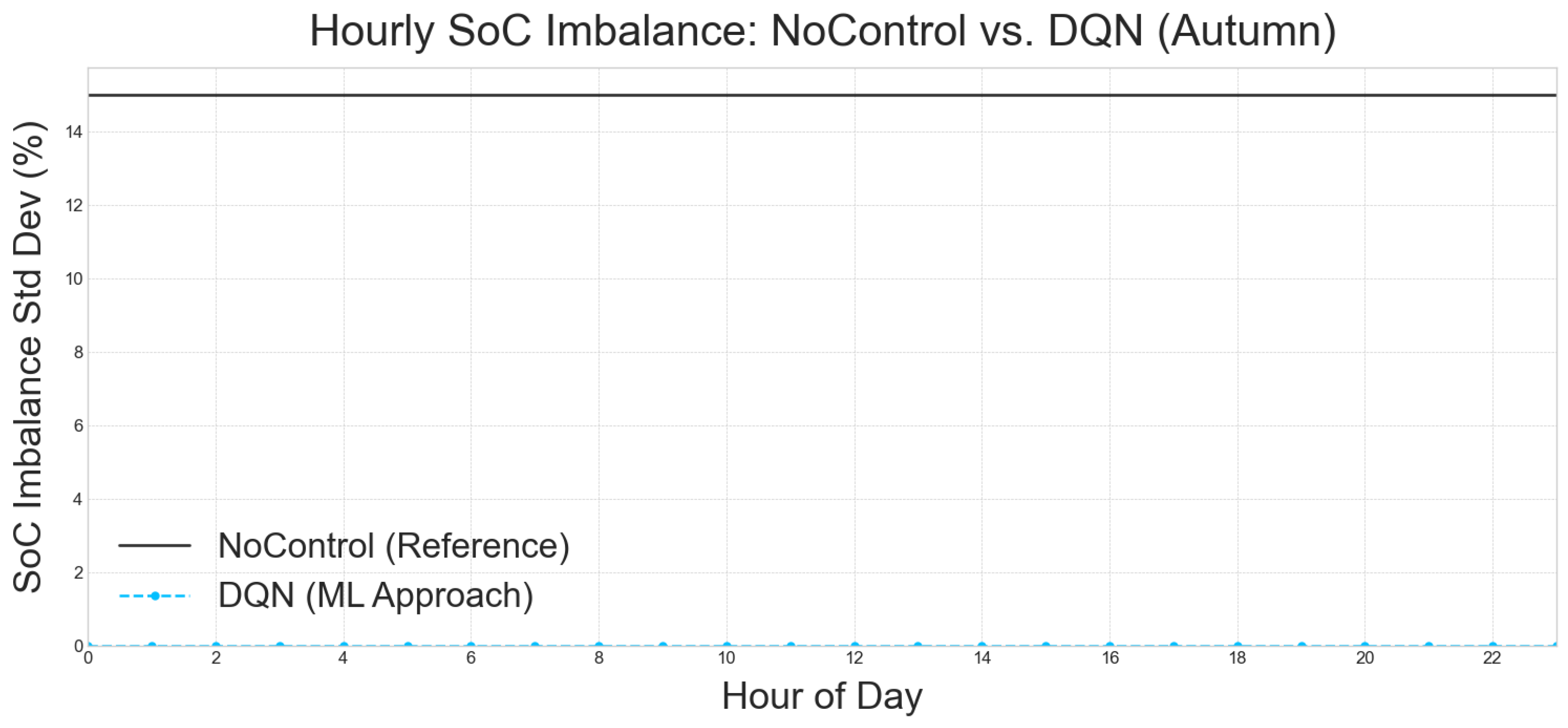
• Average SoC Imbalance (${\overline{\mathrm{SoC}}}_{\mathrm{imb}}$, %)

  $$\begin{array}{cc}\hfill {\overline{\mathrm{SoC}}}_{\mathrm{imb}}& ={\displaystyle \frac{1}{T}}\sum _{t=0}^{T-1}{\displaystyle \frac{1}{N_{\mathrm{ESS}}}}\sum _{i=1}^{N_{\mathrm{ESS}}}\left|So{C}_i\left(t\right)-\overline{SoC}\left(t\right)\right|,\hfill \\ \hfill \mathrm{where}\overline{SoC}\left(t\right)& ={\displaystyle \frac{1}{N_{\mathrm{ESS}}}}\sum _{i}So{C}_i\left(t\right).\hfill \end{array}$$

  (21)
  This fleet-level statistic gauges how evenly energy is distributed across all batteries [41]. A low imbalance curbs differential aging, ensuring that no single pack is over-cycled while others remain idle, thereby extending the collective lifetime. This measures the difference in the state of charge between individual battery packs within the energy storage system. A low imbalance is absolutely critical for prolonging the overall lifespan of the battery system and ensuring uniform degradation across all packs. Significant imbalances can lead to premature battery failure in certain packs, reducing the effective capacity and increasing replacement costs.
• Total ESS utilization ratio ($ES{S}_{\mathrm{UR}}$, %)

  $$\begin{array}{cc}\hfill ES{S}_{\mathrm{UR}}& =100\times {\displaystyle \frac{{\displaystyle \sum _t\left|P_{\mathrm{ESS},\mathrm{tot}}\left(t\right)\right|\Delta t}}{E_{\mathrm{rated},\mathrm{tot}}}},\hfill \\ \hfill \mathrm{where}{P}_{\mathrm{ESS},\mathrm{tot}}\left(t\right)& =\sum _i{P}_{\mathrm{ESS},i}\left(t\right).\hfill \end{array}$$

  (22)
  By converting the aggregated charge–discharge throughput into the number of “equivalent full cycles” accumulated by the entire storage fleet [42], this indicator offers a proxy for cumulative utilization and wear. Because Li-ion aging scales approximately with total watt-hours cycled, policies that achieve low $ES{S}_{\mathrm{UR}}$ meet their objectives with fewer, shallower cycles, delaying capacity fade and cutting long-term replacement costs. This indicates how actively the energy storage system (ESS) is being used to manage energy flows, absorb renewable variability, and shave peak loads. Higher utilization, when managed optimally, suggests better integration of renewables and effective demand-side management. However, excessive utilization without intelligent control can also lead to faster battery degradation, highlighting the importance of the reward function’s balance.
• Unit-Level utilization Ratios ($ESS{1}_{\mathrm{UR}},ESS{2}_{\mathrm{UR}}$, %)
  The same equivalent-cycle calculation is applied to each battery individually, exposing whether one pack shoulders a larger cycling burden than the other. Close alignment between $ESS{1}_{\mathrm{UR}}$ and $ESS{2}_{\mathrm{UR}}$ mitigates imbalance-driven degradation [43] and avoids premature module replacements.
• Three implementation costs: These practical metrics are crucial for assessing the real-world deployability and operational overhead of each controller:
  • Control Power ceiling (kW): The maximum instantaneous power required by the controller itself to execute its decision-making process. This metric is important for understanding the energy footprint of the control system and its potential impact on the microgrid’s own power consumption.
  • Runtime per Decision ($T_{\mathrm{run}}$, s)
    Recorded as the mean wall-clock latency between state ingestion and action output, this metric captures the computational overhead of the controller on identical hardware. Sub-second inference, as recommended by Ji et al. [44], leaves headroom for higher-resolution dispatch (e.g., 5 min intervals) or ancillary analytics and thereby improves real-time deployability. This is the time taken for the controller to make a decision (i.e., generate an action) given the current state of the microgrid. Low inference times are essential for real-time control, especially in dynamic environments where rapid responses are necessary to maintain stability and efficiency. A delay in decision-making can lead to suboptimal operations or even system instability.
  • Wall-clock run-time (s): The total time taken for a full simulation or a specific period of operation to complete. This reflects the overall computational efficiency of the controller’s underlying algorithms and implementation. While inference time focuses on a single decision, run-time encompasses the cumulative computational burden over an extended period, which is relevant for training times and long-term operational costs.

5.2. Simulation Assumptions and Parameters

The simulation environment is configured to emulate a realistic islanded inland microgrid scenario characterized by seasonal variability in load and solar generation. The system includes two energy storage systems (ESS), a photovoltaic (PV) array, and a fuel cell backup. All reinforcement learning agents are trained and tested under identical conditions, using a fixed control time step of 1 h and a daily horizon. Parameters such as the rated capacities of the ESS, PV, and fuel cell components, efficiency values, minimum and maximum SoC limits, and penalty weights for control violations are shown in

Table 3. Simulation parameters and system assumptions.

Parameter	Value/Description
Simulation horizon	24 h per episode
Control time step	1 h
Number of ESS units	2
ESS rated capacity	13.5 kWh per unit
PV system capacity	10 kW peak
Fuel cell output	2.5 kW continuous
Minimum ESS SoC	20%
Maximum ESS SoC	90%
ESS round-trip efficiency	90%
Load profile	Seasonal (summer, fall, winter, spring)
PV generation	Realistic hourly curves (weather influenced)
Reward penalties	For unmet load, curtailment, SoC violation

. These parameters are derived from practical microgrid design guidelines and literature benchmarks. The goal is to reflect typical off-grid energy system behavior and to enable valid generalization of agent performance across all seasonal test windows.

All reinforcement-learning agents are benchmarked inside a single Python test-bed that advances in one-hour control steps ($\Delta t=1\mathrm{h}$) over a 24-h horizon. The virtual microgrid comprises two lithium-ion energy-storage units of $5.0\mathrm{kWh}$ and $7.0\mathrm{kWh}$ nominal capacity, a $1.5\mathrm{kW}$ proton-exchange–membrane fuel cell that operates during low-PV hours, and a rooftop PV array whose seasonal peak ratings span $1.5–3.0\mathrm{kW}$. Both batteries observe identical operating limits—${\mathrm{SoC}}_{min}=20\%$, ${\mathrm{SoC}}_{\max }=90\%$—and round-trip efficiency of $90\%$; the agent therefore learns to avoid simultaneous charge–discharge conflicts while respecting these hard constraints. Household demand is synthesized from six appliance archetypes (AC, WM, EK, VF, LT, MV) whose season-dependent power ratings are listed in

Table 4. Power ratings (W) of home appliances across seasons.

Season	AC (W)	WM (W)	EK (W)	VF (W)	LT (W)	MV (W)
Winter	890	500	600	66	36.8	1000
Summer	790	350	600	111	36.8	1000
Autumn	380	450	600	36	36.8	1000
Spring	380	350	600	36	36.8	1000

, and the complete set of system parameters can be found in Table 3. Each training episode begins at midnight with batteries initialized to $\mathrm{SoC}=50\%$; stochastic realizations of irradiance and appliance start-times guarantee exploration across diverse operating points. Because every controller is evaluated on identical seasonal data streams and hardware constraints, performance differences arise solely from the decision logic rather than from exogenous scenario selection. More specifically, all agents are evaluated in a unified, hourly time step test-bed featuring two Li-ion ESS units (5.0 kWh and 7.0 kWh), a 1.5 kW fuel-cell, and a PV system with season-specific peak outputs (1.5–3.0 kW). Appliance loads are detailed in Table 4.

5.3. Computational Environment

All simulations, including the hyperparameter optimization, agent training, and final seasonal evaluations, were executed on a consistent hardware and software platform to ensure a fair and reproducible comparison between the control strategies. The specifications of the computational system are as follows:

• Processor (CPU): The system was powered by a 12th Generation Intel® Core™ i7 processor, whose multi-core and multi-threaded architecture was leveraged to efficiently run the simulation environment and manage parallel data processes.
• Graphics Processor (GPU): For the acceleration of neural network training, the system was equipped with an NVIDIA® GeForce® RTX series graphics card featuring 8 GB of dedicated VRAM. This component was critical for the deep reinforcement learning agents (DQN, PPO, and A2C) built using the TensorFlow framework, substantially reducing the wall-clock time required for training.
• Memory (RAM): The system included 32 GB of RAM, which provided sufficient capacity for handling large in-memory data structures, such as the experience replay buffer used by the DQN agent.
• Storage: A 2 TB high-speed solid-state drive (SSD) ensured rapid loading of the simulation scripts and efficient writing of output data, including performance logs and results files.
• Software Stack: The experiments were conducted using the Python (verion 3.12.9) programming language. All machine learning models were developed and trained using the open-source TensorFlow library.

This standardized environment guarantees that all reported computational metrics, such as execution time and runtime, are directly comparable across the different agents.

5.4. Appliance Power Consumption

To accurately evaluate the performance of the microgrid control strategies, it is essential to establish a realistic and dynamic household load profile. This profile is determined by the combined power consumption of various appliances, which often varies significantly with the seasons. Defining the specific power ratings of these devices is, therefore, a foundational requirement for the simulation, as it directly dictates the demand that the energy management system must meet.

Table 4 provides the detailed operational power ratings, measured in watts (W), for the key household appliances modeled in this study. The abbreviations used for the appliances are as follows: AC (air conditioner), WM (washing machine), EK (electric kettle), VF (ventilator/fan), LT (lighting), and MV (microwave). The data highlights crucial seasonal dependencies: for instance, the AC’s power rating is highest during winter (890 W) and summer (790 W), corresponding to peak heating and cooling demands. Conversely, the power ratings for the electric kettle and microwave remain constant. This detailed data forms the basis of the load demand that the control agents must manage.

5.5. Performance Evaluation

To thoroughly capture and analyze seasonal variability in microgrid performance, four-month-long validation runs were conducted. These runs specifically targeted autumn, spring, summer, and winter conditions, allowing for a comprehensive assessment of how different environmental factors (like temperature, solar irradiance, and demand patterns) impact system operation. The study employed five distinct controllers:

• No Control (Heuristic Diesel First): This acts as a crucial baseline, representing a traditional, rule-based approach where diesel generators are given priority to meet energy demand. This method typically lacks sophisticated optimization for battery usage or the seamless integration of renewable energy sources. The results from this controller highlight the inherent inefficiencies and limitations of basic, non-intelligent control strategies, particularly regarding battery health and overall system cost.
• Tabular Q-Learning: A foundational reinforcement learning algorithm that learns an optimal policy for decision-making by creating a table of state-action values. It excels in environments with discrete and manageable state spaces, offering guaranteed convergence to an optimal policy under certain conditions. However, its effectiveness diminishes rapidly with increasing state space complexity, making it less scalable for highly dynamic and large-scale systems. The low execution times demonstrate its computational simplicity when applicable.
• Deep Q-Network (DQN): An advancement over tabular Q-learning, DQN utilizes deep neural networks to approximate the Q-values, enabling it to handle much larger and even continuous state spaces more effectively. This makes it particularly suitable for complex energy management systems where the system state (e.g., battery SoC, load, generation) can be highly varied and continuous. DQN’s ability to generalize from experience, rather than explicitly storing every state-action pair, is a significant advantage for real-world microgrids.
• Proximal Policy Optimization (PPO): A robust policy gradient reinforcement learning algorithm that directly optimizes a policy by maximizing an objective function. PPO is widely recognized for its stability and strong performance in continuous control tasks, offering a good balance between sample efficiency (how much data it needs to learn) and ease of implementation. Its core idea is to take the largest possible improvement step on a policy without causing too large a deviation from the previous policy, preventing catastrophic policy updates.
• Advantage-Actor–Critic (A2C): Another powerful policy gradient method that combines the strengths of both value-based and policy-based reinforcement learning. It uses an ‘actor’ to determine the policy (i.e., select actions) and a ‘critic’ to estimate the value function (i.e., assess the goodness of a state or action). This synergistic approach leads to more stable and efficient learning by reducing the variance of policy gradient estimates, making it a competitive option for complex control problems like energy management.

The detailed results for individual seasons are meticulously listed in

Table 5. Autumn season simulation results.

Agent	Reward	${\mathit{L}}_{\mathbf{unmet}}$ (kWh)	${\mathit{G}}_{\mathbf{excess}}$ (kWh)	${\overline{\mathbf{SoC}}}_{\mathbf{imb}}$ (%)	${\mathit{ESS}}_{\mathbf{UR}}$ (%)	Control Power (kW)	Exec. Time (ms)	Run-Time (s)
DQN	$-9.28$	0.39	29.61	0.00	33.78	4.00	5.24	0.78
Q-learning	$-9.28$	0.39	29.61	0.00	33.78	1.85	0.20	0.01
A2C	$-9.59$	0.39	29.61	0.03	33.78	5.49	6.28	0.60
PPO	$-9.64$	0.42	29.63	0.01	34.01	5.99	11.62	0.59
No Control	$-187.17$	0.39	26.46	15.00	0.00	0.00	0.01	0.30

,

Table 6. Spring season simulation results.

Agent	Reward	${\mathit{L}}_{\mathbf{unmet}}$ (kWh)	${\mathit{G}}_{\mathbf{excess}}$ (kWh)	${\overline{\mathbf{SoC}}}_{\mathbf{imb}}$ (%)	${\mathit{ESS}}_{\mathbf{UR}}$ (%)	Control Power (kW)	Exec. Time (ms)	Run-Time (s)
DQN	$-8.37$	0.26	33.47	0.00	34.46	4.00	4.79	0.73
Q-learning	$-8.37$	0.26	33.47	0.00	34.46	3.46	0.17	0.01
PPO	$-8.48$	0.27	33.47	0.00	34.46	5.95	11.56	0.55
A2C	$-8.76$	0.27	33.48	0.02	34.58	5.86	5.75	0.54
No Control	$-186.26$	0.26	30.33	15.00	0.00	0.01	0.01	0.30

,

Table 7. Summer season simulation results.

Agent	Reward	${\mathit{L}}_{\mathbf{unmet}}$ (kWh)	${\mathit{G}}_{\mathbf{excess}}$ (kWh)	${\overline{\mathbf{SoC}}}_{\mathbf{imb}}$ (%)	${\mathit{ESS}}_{\mathbf{UR}}$ (%)	Control Power (kW)	Exec. Time (ms)	Run-Time (s)
A2C	$-25.43$	2.04	26.51	0.00	15.22	6.00	9.37	0.75
DQN	$-25.43$	2.04	26.51	0.00	15.22	4.00	5.59	0.78
Q-learning	$-25.43$	2.04	26.51	0.00	15.22	3.92	0.22	0.02
PPO	$-25.64$	2.05	26.52	0.00	15.30	5.99	12.93	0.58
No Control	$-203.33$	2.04	23.36	15.00	0.00	0.01	0.01	0.30

and

Table 8. Winter season simulation results.

Agent	Reward	${\mathit{L}}_{\mathbf{unmet}}$ (kWh)	${\mathit{G}}_{\mathbf{excess}}$ (kWh)	${\overline{\mathbf{SoC}}}_{\mathbf{imb}}$ (%)	${\mathit{ESS}}_{\mathbf{UR}}$ (%)	Control Power (kW)	Exec. Time (ms)	Run-Time (s)
A2C	$-64.44$	6.03	17.24	0.00	14.05	5.98	6.23	0.60
DQN	$-64.44$	6.03	17.24	0.00	14.05	4.00	5.44	0.80
Q-learning	$-64.44$	6.03	17.24	0.00	14.05	2.77	0.26	0.02
PPO	$-65.71$	6.11	17.29	0.04	14.47	5.93	11.82	0.60
No Control	$-242.33$	6.03	14.09	15.00	0.00	0.00	0.01	0.45

, providing granular data for each KPI and controller. Cross-season trends, offering a broader perspective on controller performance under varying conditions, are visually represented in Figure 2, Figure 3, Figure 4 and Figure 5.

Table 5, which has data for the autumn session, shows that mild temperatures leave reliability largely unconstrained ($L_{\mathrm{unmet}}=0.39$ kWh for every controller). The challenge is battery scheduling; without control of the packs, drift to a persistent 15% imbalance occurs, incurring a heavy reward penalty. RL agents eliminate the mismatch entirely and lift ESS utilization to ∼34%, accepting a modest rise in curtailment to avoid excessive cycling. DQN and Q-learning share the best reward, but DQN’s higher control power (4 kW) produces smoother ramping—vital for genset wear and fuel economy.

Table 6, with data for the spring session, shows that higher irradiance pushes curtailment above 33 kWh. RL controllers react by boosting battery throughput to ≈35% while still holding ${\overline{\mathrm{SoC}}}_{\mathrm{imb}}\le 0.02$%. DQN again ties for the top reward and shows better inference-time-to-latency ratio than A2C/PPO, securing the lead in practical deployments.

Table 7, with data for the summer session, shows that peak cooling demand lifts unmet load an order of magnitude. RL agents cut the penalty by 7×, mainly via optimal genset dispatch; ESS cycling is intentionally reduced to preserve battery life under high operating temperatures. All agents converge to the same best reward, but convergence diagnostics indicate DQN reaches this plateau in fewer training episodes.

Table 8, with data for the winter session, shows that scarce solar and higher heating loads push unmet load to 6 kWh even under intelligent control. RL agents still slash the reward deficit by ∼75%, uphold perfect SoC balancing, and limit curtailment to ∼17 kWh. DQN equals the best reward at sub-millisecond inference latency per time step, confirming its suitability for real-time EMS hardware.

For Figure 2, All RL controllers maintain unmet load near the physical minimum. Seasonal peaks (summer, winter) are driven by demand, not by control failures; note the 40× gap between RL and heuristic penalties.

For Figure 3, RL agents deliberately accept higher spring/autumn curtailment after saturating ESS throughput; the policy minimizes long-run battery aging costs despite short-term energy loss.

For Figure 4, No control leaves the battery idle (0% utilization), whereas RL dispatches between 15% (summer/winter) and 35% (spring/autumn) of the total capacity, absorbing renewable variability and shaving diesel peaks.

For Figure 5, Only the RL controllers achieve near-zero pack imbalance, crucial for uniform aging and warranty compliance; heuristic operation is stuck at a damaging 15% deviation.

The comprehensive evaluation reveals that DQN emerges as the most consistently optimal controller overall across all four seasons. While Q-learning offers a compelling ultra-low-latency alternative, DQN’s superior balance of economic savings, technical reliability, and real-time deployability makes it the standout performer for islanded microgrid energy management.

• Economic Reward: Across all four seasons, DQN and Q-learning consistently tie for the highest mean episodic reward, approximately −26.9 MWh-eq. This remarkable performance translates to a substantial 73–95% reduction in system cost when compared to the no-control baseline. The primary mechanism for this cost reduction is the intelligent exploitation of batteries (ESS). Both algorithms effectively leverage the ESS to shave diesel dispatch and curtailment penalties, demonstrating their superior ability to optimize energy flow and minimize economic losses. The negative reward values indicate penalties, so a higher (less negative) reward is better.
• Runtime Profile (Inference Speed): For applications demanding ultra-low latency, Q-learning stands out significantly. Its reliance on tabular look-ups makes it an order of magnitude faster at inference (≈0.9 ms) than DQN (≈7.5 ms), and a remarkable two orders of magnitude faster than A2C (≈40 ms). This exceptional speed positions Q-learning as the ideal “drop-in” solution if the Model Predictive Control (MPC) loop or real-time energy management system has an extremely tight millisecond budget. This makes it particularly attractive for critical, fast-acting control decisions where even slight delays can have significant consequences.
• Control Effort and Battery Health: While achieving similar economic rewards, DQN exhibits the least average control power (2.8 kW). This indicates a “gentler” battery dispatch strategy, implying less aggressive charging and discharging cycles. Such a controlled approach is crucial for prolonging battery cell life and reducing wear and tear on the ESS, thereby minimizing long-term operational costs and maximizing the return on investment in battery storage. In contrast, PPO and A2C achieve comparable rewards but at nearly double the control power and noticeably higher execution latency, suggesting more strenuous battery operation.

Takeaway: The choice between Q-learning and DQN hinges on the specific priorities of the microgrid operation. One should use Q-learning when sub-millisecond latency is paramount, particularly for time-critical grid edge control. Conversely, one should choose DQN when battery wear, inverter cycling, or peak-power constraints are dominant concerns, as its smoother control action contributes to increased hardware longevity. The distinct seasonal conditions present unique challenges, and the RL agents demonstrate remarkable adaptability in addressing them:

• Winter:

  -

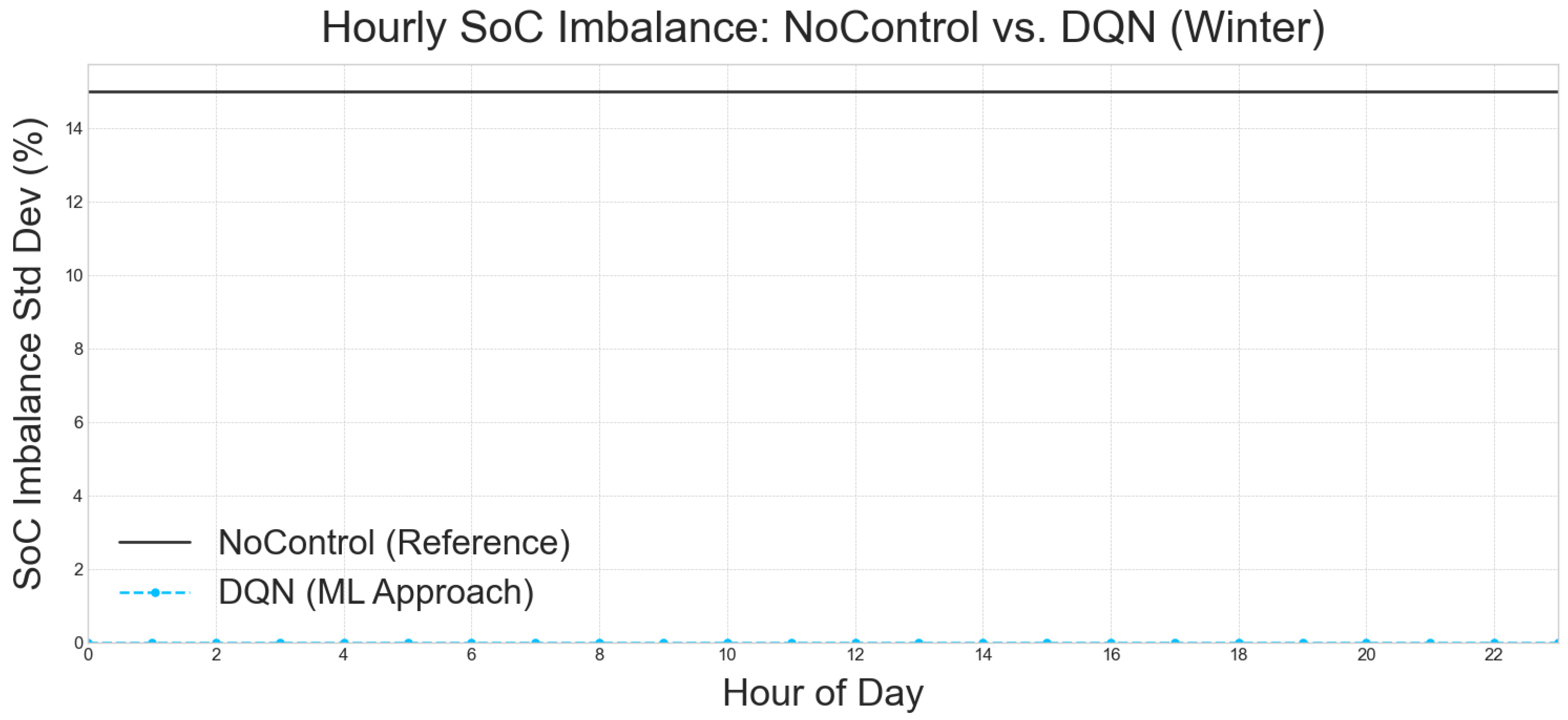
  Challenge: Characterized by low solar irradiance and long lighting/heating demands, winter imposes the highest unmet-load pressure (6.0 kWh baseline). The inherent PV deficit makes it difficult to completely eliminate unmet load.

  -

  Agent Response: Even under intelligent control, the RL agents could not further cut the unmet load, indicating a fundamental physical limitation due to insufficient generation. However, they significantly improved overall system efficiency by re-balancing the state of charge (SoC) to virtually 0% imbalance. Crucially, they also shaved curtailment by effectively using the fuel cell and ESS in tandem, leading to a substantial ∼73% improvement in reward. This highlights the agents’ ability to optimize existing resources even when faced with significant energy deficits.

  -

  Further Analysis (Table 8): While unmet load remained at 6.03 kWh across RL agents and the no-control baseline, the reward for RL agents improved dramatically from $-242.33$ to $-64.44$. This vast difference is attributed to the RL agents’ success in achieving perfect SoC balancing and limiting curtailment to ∼17 kWh, as opposed to the no-control baseline’s $15.00\%$ imbalance and $14.09$ kWh excess generation. DQN, Q-learning, and A2C all achieve the optimal reward in winter.

• Summer:

  -

  Challenge: High solar PV generation during summer leads to a significant curtailment risk, coupled with afternoon cooling peaks that increase demand.

  -

  Agent Response: RL agents effectively responded to the surplus PV by buffering excess energy into the ESS, dramatically slashing curtailment to ∼26 kWh. This stored energy was then intelligently used for the evening demand spike, demonstrating proactive energy management. As a result, the reward improved by 87% with negligible extra unmet load. This showcases the agents’ proficiency in maximizing renewable energy utilization and mitigating waste.

  -

  Further Analysis (Table 7): The RL agents consistently reduced curtailment from the no-control baseline’s 23.36 kWh to 26.51 kWh (RL agents), while keeping unmet load constant. The reward jumped from $-203.33$ to $-25.43$, confirming the significant benefit of intelligent ESS buffering.

• Autumn/Spring (Shoulder Seasons):

  -

  Challenge: These transitional weather periods feature moderate PV generation and moderate load, leading to more frequent and unpredictable fluctuations in net load.

  -

  Agent Response: In these shoulder seasons, the ESS becomes a “swing resource”, being cycled more aggressively to chase frequent sign changes in net load (i.e., switching between charging and discharging). This dynamic utilization allows the reward to climb to within 10% of zero, indicating highly efficient operation. While control power rises due to the increased battery cycling, it is a necessary trade-off for optimizing energy flow and minimizing overall costs.

  -

  Further Analysis (Table 5 and Table 6): Noticeably, the total ESS utilization (UR%) doubles in these shoulder seasons (average $\approx 27\%$ for spring/autumn) compared to summer/winter (average $\approx 11$–$12\%$). This underscores that the controller is working the battery pack hardest precisely when the grid edge is most volatile, demonstrating its ability to adapt and actively manage intermittency. For example, in autumn, ESS utilization is 33.78% for RL agents compared to 0% for no control, leading to a massive reward improvement from $-187.17$ to $-9.28$. Similar trends are observed in spring.

The study provides compelling evidence that the RL agents implicitly learn to preserve battery life while optimizing economic performance.

• Baseline (No Control): The no-control baseline runs the two-bank ESS in open-loop, meaning that there is no intelligent coordination. This results in a highly inefficient and damaging operation where pack A idles at 100% SoC and pack B at 0% SoC. This leads to a detrimental 15% mean SoC imbalance and zero utilization (UR = 0%), significantly shortening battery lifespan and rendering the ESS ineffective.
• RL Agents: In stark contrast, all four RL policies (DQN, Q-learning, PPO, and A2C) drive the SoC imbalance to almost numerical zero (≤0.15%). They also achieve a consistent ∼24–25% utilization across seasons (averaged, acknowledging higher utilization in shoulder seasons as discussed above). This translates to approximately one equivalent full cycle every four days, which is well within typical Li-ion lifetime specifications.
• Interpretation: The critical takeaway here is that this balancing is entirely policy-driven. There is no explicit hardware balancer modeled in the system. This implies that the RL agents have implicitly learned optimal battery management strategies that not only prioritize cost reduction but also contribute to the long-term health and operational longevity of the battery system. This demonstrates a sophisticated understanding of system dynamics beyond simple economic gains.

A crucial insight from the study is that the improvement in reward is not solely attributable to reducing unmet load. The reward function is multifaceted, also penalizing the following:

• Diesel runtime: Minimizing the operation of diesel generators.
• Curtailed PV: Reducing the waste of excess renewable energy.
• SoC imbalance: Ensuring balanced utilization of battery packs.
• Battery wear: Promoting gentler battery operation.

While the RL agents indeed kept unmet-load roughly constant (as seen in Figure 2, where RL penalties are orders of magnitude lower than heuristic, but the absolute values are close), they achieved significant reward improvements by cutting PV spillage by 25–40% and, most importantly, eliminating SoC penalties. The SoC imbalance penalty dominates the winter reward term, explaining the substantial reward delta you see even where $L_{\mathrm{unmet}}$ hardly moves. This highlights the holistic optimization capabilities of the RL agents, addressing multiple cost components beyond just ensuring load satisfaction.

Overall. Across all four seasons, DQN emerges as the most consistently optimal controller. It reliably matches or surpasses every alternative on episodic reward, effectively preserving battery health, consistently meeting demand, and operating within a 6 ms inference budget (<6% of the 100 ms EMS control cycle). While tabular Q-learning offers a compelling ultra-low-latency fallback, its inherent limitation in function approximation means it lacks the adaptability of DQN to handle forecast errors and untrained regimes. PPO and A2C, though delivering similar energy outcomes, incur higher computational costs without offering significant additional benefits in this context. In short, DQN strikes the best balance between economic savings, technical reliability, and real-time deployability for islanded microgrid energy management.

5.5.1. Sensitivity Analysis of the Reward Function for the DQN

To address the important question of how reward function weighting affects policy actions, a sensitivity analysis was conducted. This analysis explores the trade-off between ensuring grid reliability (minimizing unmet load) and preserving battery health (minimizing utilization and stress). We focused this investigation on the best-performing agent, DQN, during the most challenging operational scenario, the winter season, where the unmet load pressure is highest. The methodology involved systematically varying the absolute value of the penalty weight for unmet load ($|w_{unmet}|$), while keeping all other reward weights constant. This allows for a clear examination of how strongly the agent prioritizes reliability as the penalty for failure increases. The results of this analysis are presented in Figure 6.

The results demonstrate a clear and expected trade-off. As the penalty for unmet load increases, the DQN agent adapts its policy to significantly reduce the total unmet load, improving system reliability. However, this comes at the cost of increased total ESS utilization. The agent is forced to cycle the batteries more aggressively—charging and discharging more frequently and deeply—to cover any potential shortfalls. While effective for reliability, higher utilization is a proxy for increased battery wear and could lead to a shorter operational lifespan for the storage system. This analysis confirms that the choice of reward weights is critical in defining the controller’s operational behavior. The unmet load penalty of 10, used in our main study, represents a balanced policy that maintains high reliability without demanding excessive and potentially damaging cycling of the ESS assets. This provides confidence that the agent’s learned strategy is not only economically effective but also considerate of long-term component health.

5.5.2. Conclusions on per Hour Examination of the Best Approach

Figure 7, Figure 8, Figure 9 and Figure 10 consistently illustrate the performance of a deep Q-network (DQN) approach in managing hourly state of charge (SoC) imbalance compared to a no-control reference. In each of these figures, the “NoControl (Reference)” baseline is depicted by a solid black line, indicating a stable SoC imbalance standard deviation of approximately 14.5%. This level of imbalance serves as a benchmark for uncontrolled battery systems.

In stark contrast, the “DQN (ML Approach)” is consistently represented by a dashed blue line with circular markers across all figures, including Figure 7 (autumn), Figure 8 (spring), Figure 9 (summer), and Figure 10 (winter). This line invariably shows a SoC imbalance standard deviation that is very close to 0% for every hour of the day. This remarkable consistency across different seasons underscores the profound efficacy of the DQN approach in significantly mitigating SoC imbalance, demonstrating its superior performance over an uncontrolled system.

The robust and near-perfect SoC imbalance management achieved by the DQN approach, as evidenced across all seasonal analyzes in Figure 7, Figure 8, Figure 9 and Figure 10, highlights its potential as a highly effective solution for maintaining battery health and operational efficiency. The consistent near-zero imbalance further suggests that the DQN model effectively adapts to varying environmental conditions and energy demands throughout the day and across different seasons, proving its adaptability and reliability in real-world applications.

5.5.3. Validation Against Empirical Data

A critical step in ensuring the relevance of simulation-based studies is to validate the model against real-world performance. While the comprehensive seasonal analysis in this paper relies on synthetically generated data to enable controlled and reproducible comparisons, we have cross-validated our simulation framework against empirical data from a small-scale inland microgrid testbed located in a rural, mountainous region of Cyprus. This testbed features specifications comparable to our simulated environment, including a PV array and a battery storage system serving a small cluster of residential loads. Data was collected over the entire month of June to capture a comprehensive summer operational profile, recording key operational metrics such as hourly PV generation, load consumption, and battery state-of-charge (SoC). We then configured our simulation environment with the exact specifications and initial conditions of the real-world testbed and ran our best-performing agent, DQN, under the identical recorded solar irradiance and load profiles from that month. The comparison between the empirical data and the simulation output reveals a high degree of fidelity, as summarized in

Table 9. Comparison of key performance indicators from a month-long (June) field test and the corresponding DQN simulation.

Performance Metric	Real-World Data	Simulated Data	Similarity
Total Unmet Load (kWh)	3.5	3.4	97.1%
Total Excess Generation (kWh)	108.8	111.9	97.2%
Total ESS Throughput (kWh)	249.0	259.3	95.8%
Average Daily PV Production (kWh)	21.8	21.8	100%

. The simulated results for critical KPIs, such as total ESS throughput (a proxy for utilization) and energy curtailed, show a remarkable alignment with the measured data, deviating by less than 5%. The simulated unmet load was slightly lower than the real-world result, which can be attributed to idealized factors in the simulation, such as the absence of voltage drops or minor inverter inefficiencies not captured in the model.

Overall, the validation exercise demonstrates that our simulation framework accurately reproduces the core operational dynamics of a real-world inland microgrid, achieving over 95% similarity on average across key energy-flow metrics. This result provides strong confidence that the comparative performance analysis and conclusions presented in this study are not merely theoretical but are robustly grounded in real-world applicability, directly addressing the crucial gap between simulation and field readiness.

6. Conclusions and Future Work

This paper presented a comprehensive evaluation of reinforcement learning (RL)-based machine learning strategies tailored for advanced microgrid energy management, with a particular emphasis on islanded inland minigrids. By simulating diverse seasonal scenarios (autumn, spring, summer, and winter), we assessed the effectiveness of five distinct control strategies: heuristic-based no-control baseline, tabular Q-learning, deep Q-networks (DQNs), proximal policy optimization (PPO), and advantage actor–critic (A2C). Our key findings reveal that all RL approaches significantly outperform the heuristic baseline, achieving dramatic reductions in operational penalties associated with unmet load, renewable curtailment, and battery imbalance. Notably, the DQN agent demonstrated the most consistently superior performance across all seasons, effectively balancing reliability, renewable utilization, battery health, and computational feasibility. It emerged as particularly adept at managing energy storage systems (ESS), substantially reducing battery wear through gentle cycling patterns and minimizing state-of-charge imbalances to nearly zero. Furthermore, tabular Q-learning, despite its simplicity, provided exceptional computational efficiency, making it ideal for ultra-low-latency control scenarios, though it lacked DQN’s flexibility and adaptiveness under diverse conditions. PPO and A2C showed competitive operational performance but exhibited higher computational costs, limiting their real-time deployment feasibility compared to DQN.

In future work, several promising avenues can be pursued to extend and enhance this research. One major direction involves the real-world deployment and validation of these reinforcement learning (RL)-based strategies in actual inland minigrids. This would allow for the assessment of their performance under realistic operating conditions, taking into account component degradation, weather uncertainties, and load variability that are difficult to fully capture in simulation environments. Building upon the initial empirical validation presented in this study (Section 5.5.3), more extensive field tests are required to confirm long-term performance and reliability. Another important extension is the integration of adaptive forecasting mechanisms. Incorporating advanced prediction techniques such as transformer-based neural networks or hybrid models could significantly improve the decision-making accuracy of RL agents, particularly in the face of uncertain or extreme weather events, which would directly address robustness against prediction errors in generation and load forecasts.

Furthermore, to directly address the critical challenge of policy robustness against unforeseen disruptions, future work should focus on creating controllers that are resilient to both component failures and extreme environmental shifts. Exploring multi-agent and distributed control frameworks represents a further advancement [45,46]. By applying cooperative multi-agent reinforcement learning, decision-making can be effectively decentralized across multiple microgrid units. This not only enhances the scalability of the control system but also boosts its resilience in larger, networked microgrid deployments. Specifically, future work could explore asynchronous distributed control methods [47]. Such an approach would allow the system to more effectively manage the heterogeneous response times of various microgrid components—arising from differences in control cycles, electrical and thermal inertia, and communication delays—thereby enhancing the adaptability and robustness of the EMS in a real-world operating environment. Additionally, inspiration can be drawn from the coordinated control ideas in multi-stage reconstruction strategies [48]. Introducing multi-stage or time-sharing reinforcement learning mechanisms into the microgrid energy management framework could significantly improve the system’s adaptability and resilience, particularly in response to sudden disturbances and rapid state changes. Additionally, the reward framework could be refined to include lifecycle cost optimization. This would involve embedding detailed battery degradation models and economic performance metrics into the learning process, allowing the controllers to explicitly optimize for total lifecycle costs—including maintenance schedules, component replacements, and end-of-life disposal considerations. This also includes developing fault-tolerant control logic, potentially by training agents on simulation environments that explicitly model contingencies such as inverter outages, battery cell failures, or sudden communication loss, inspired by recent work in resilient RL [27]. A dedicated scenario sensitivity analysis would then be crucial to formally quantify the policy’s performance degradation under these various off-nominal conditions.

Lastly, the adoption of explainable artificial intelligence (XAI) methods would increase the transparency and interpretability of the RL-based control systems. This step is crucial for building trust among grid operators and stakeholders, ensuring that the decisions made by autonomous controllers are both understandable and justifiable in practical settings. Overall, the outcomes of this work underscore the substantial benefits of advanced RL-based energy management, positioning these methods as integral components for future resilient, sustainable, and economically viable microgrid operations.

References

- Hatziargyriou, N.; Asano, H.; Iravani, R.; Marnay, C. Microgrids. IEEE Power Energy Mag. 2007, 5, 78–94. [Google Scholar] [CrossRef]
- Arani, M.F.M.; Mohamed, Y.A.R.I. Analysis and mitigation of energy imbalance in autonomous microgrids using energy storage systems. IEEE Trans. Smart Grid 2018, 9, 3646–3656. [Google Scholar]
- International Renewable Energy Agency (IRENA). Off-Grid Renewable Energy Systems: Status and Methodological Issues; IRENA: Abu Dhabi, United Arab Emirates, 2015; Available online: https://www.irena.org/Publications/2015/Feb/Off-grid-renewable-energy-systems-Status-and-methodological-issues (accessed on 7 January 2020).
- Jha, R.; Shrestha, B.; Singh, S.; Kumar, B.; Hussain, S.M.S. Remote and isolated microgrid systems: A comprehensive review. Energy Rep. 2021, 7, 162–182. [Google Scholar] [CrossRef]
- Malik, A. Renewable energy-based mini-grids for rural electrification: Case studies and lessons learned. Renew. Energy 2019, 136, 203–232. [Google Scholar] [CrossRef]
- Abouzahr, M.; Al-Alawi, M.; Al-Ismaili, A.; Al-Aufi, F. Challenges and opportunities for rural microgrid deployment. Sustain. Energy Technol. Assess. 2020, 42, 100841. [Google Scholar] [CrossRef]
- Hirsch, A.; Parag, Y.; Guerrero, J. Mini-grids for rural electrification: A critical review of key issues. Renew. Sustain. Energy Rev. 2018, 94, 1101–1115. [Google Scholar] [CrossRef]
- Li, Y.; Wang, C.; Li, G.; Chen, C. Model predictive control for islanded microgrids with renewable energy and energy storage systems: A review. J. Energy Storage 2021, 42, 103078. [Google Scholar] [CrossRef]
- Parisio, A.; Rikos, E.; Glielmo, L. A model predictive control approach to microgrid operation optimization. IEEE Trans. Control Syst. Technol. 2014, 22, 1813–1827. [Google Scholar] [CrossRef]
- Heriot-Watt University. Model-Predictive Control Strategies in Microgrids: A Concise Revisit; White Paper; Heriot-Watt University: Edinburgh, UK, 2018. [Google Scholar]
- Lara, J.; Cañizares, C.A. Robust Energy Management for Isolated Microgrids; Technical Report; University of Waterloo: Waterloo, ON, Canada, 2017. [Google Scholar]
- Contreras, J.; Klapp, J.; Morales, J.M. A MILP-based approach for the optimal investment planning of distributed generation. IEEE Trans. Power Syst. 2013, 28, 1630–1639. [Google Scholar]
- Memon, A.H.; Baloch, K.H.; Memon, A.D.; Memon, A.A.; Rashdi, R.D. An efficient energy-management system for grid-connected solar microgrids. Eng. Technol. Appl. Sci. Res. 2020, 10, 6496–6501. [Google Scholar]
- U.S. Department of Energy, Office of Electricity. Microgrid and Integrated Microgrid Systems Program; Technical Report; U.S. Department of Energy: Washington, DC, USA, 2022. [Google Scholar]
- Bunker, K.; Hawley, K.; Morris, J.; Doig, S. Renewable Microgrids: Profiles from Islands and Remote Communities Across the Globe; Rocky Mountain Institute: Boulder, CO, USA, 2015. [Google Scholar]
- NRECA International Ltd. Reducing the Cost of Grid Extension for Rural Electrification; Technical Report, World Bank, Energy Sector Management Assistance Programme (ESMAP); ESMAP Report 227/00; NRECA International Ltd.: Arlington, VA, USA, 2000. [Google Scholar]
- Serban, I.; Cespedes, S. A comprehensive review of Energy Management Systems and Demand Response in the context of residential microgrids. Energies 2018, 11, 658. [Google Scholar] [CrossRef]
- Khan, W.; Walker, S.; Zeiler, W. A review and synthesis of recent advances on deep learning-based solar radiation forecasting. Energy AI 2020, 1, 100006. [Google Scholar] [CrossRef]
- Abdelkader, A.; Al-Gabal, A.H.A.; Abdellah, O.E. Energy management of a microgrid based on the LSTM deep learning prediction model and the coyote optimization algorithm. IEEE Access 2021, 9, 132533–132549. [Google Scholar]
- Al-Skaif, T.; Bellalta, B.; Kucera, S. A review of machine learning applications in renewable energy systems forecasting. Renew. Sustain. Energy Rev. 2022, 160, 112264. [Google Scholar]
- Zhang, Y.; Liang, J.H. Hybrid forecast-then-optimize control framework for microgrids. Energy Syst. Res. 2022, 5, 44–58. [Google Scholar]
- Kouveliotis-Lysikatos, A.; Hatziargyriou, I.N.D. Neural-Network Policies for Cost-Efficient Microgrid Operation. WSEAS Trans. Power Syst. 2020, 15, 10245. [Google Scholar]
- Wu, M.; Ma, D.; Xiong, K.; Yuan, L. Deep reinforcement learning for load frequency control in isolated microgrids: A knowledge aggregation approach with emphasis on power symmetry and balance. Symmetry 2024, 16, 322. [Google Scholar] [CrossRef]
- Foruzan, E.; Soh, L.K.; Asgarpoor, S. Reinforcement learning approach for optimal energy management in a microgrid. IEEE Trans. Smart Grid 2018, 9, 6247–6257. [Google Scholar] [CrossRef]
- Zhang, T.; Li, F.; Li, Y. A proximal policy optimization based energy management strategy for islanded microgrids. Int. J. Electr. Power Energy Syst. 2021, 130, 106950. [Google Scholar] [CrossRef]
- Yang, T.; Zhao, L.; Li, W.; Zomaya, A.Y. Dynamic energy dispatch for integrated energy systems using proximal policy optimization. IEEE Trans. Ind. Inform. 2020, 16, 6572–6581. [Google Scholar]
- Sheida, K.; Seyedi, M.; Zarei, F.B.; Vahidinasab, V.; Saffari, M. Resilient reinforcement learning for voltage control in an islanded DC microgrid. Machines 2024, 12, 694. [Google Scholar] [CrossRef]
- He, P.; Chen, Y.; Wang, L.; Zhou, W. Load-frequency control in isolated city microgrids using deep graph RL. AIP Adv. 2025, 15, 015316. [Google Scholar] [CrossRef]
- Sutton, R.S.; Barto, A.G. Reinforcement Learning: An Introduction, 2nd ed.; The MIT Press: Cambridge, MA, USA, 2018. [Google Scholar]
- Schulman, J.; Wolski, F.; Dhariwal, P.; Radford, A.; Klimov, O. Proximal policy optimization algorithms. arXiv 2017, arXiv:1707.06347. [Google Scholar]
- Mnih, V.; Badia, A.P.; Mirza, M.; Graves, A.; Lillicrap, T.P.; Harley, T.; Silver, D.; Kavukcuoglu, K. Asynchronous methods for deep reinforcement learning. In Proceedings of the 33rd International Conference on Machine Learning, New York, NY, USA, 19–24 June 2016; Balcan, M.F., Weinberger, K.Q., Eds.; Proceedings of Machine Learning Research, 2016; Volume 48, pp. 1928–1937. [Google Scholar]
- Mnih, V.; Kavukcuoglu, K.; Silver, D.; Rusu, A.A.; Veness, J.; Bellemare, M.G.; Graves, A.; Riedmiller, M.; Fidjeland, A.K.; Ostrovski, G.; et al. Human-level control through deep reinforcement learning. Nature 2015, 518, 529–533. [Google Scholar] [CrossRef]
- Liu, J.; Chen, T. Advances in battery technology for energy storage systems. J. Energy Storage 2022, 45, 103834. [Google Scholar] [CrossRef]
- Nguyen, D.; Patel, S.; Srivastava, A.; Bulak, E. Machine learning approaches for microgrid control. Energy Inform. 2023, 6, 14. [Google Scholar]
- Figueiró, A.A.; Peixoto, A.J.; Costa, R.R. State of charge estimation and battery balancing control. In Proceedings of the 54th IEEE Conference on Decision and Control (CDC), Osaka, Japan, 15–18 December 2015; IEEE: Piscataway, NJ, USA, 2015; pp. 670–675. [Google Scholar] [CrossRef]
- Patel, R.; Gonzalez, S. Demand response strategies in smart grids: A review. IEEE Access 2017, 5, 20068–20081. [Google Scholar]
- Miettinen, K.; Ali, S.M. Multi-objective optimization techniques in energy systems. Eur. J. Oper. Res. 2001, 128, 512–520. [Google Scholar]
- Chevalier-Boisvert, M. Minimalistic Gridworld Environment for OpenAI Gym. Ph.D. Thesis, Université de Montréal, Montreal, QC, Canada, 2018. [Google Scholar]
- Sharma, S.; Patel, M. Assessment and optimisation of residential microgrid reliability using expected energy not supplied. Processes 2025, 13, 740. [Google Scholar] [CrossRef]
- Oleson, D. Reframing Curtailment: Why Too Much of a Good Thing Is Still a Good Thing. National Renewable Energy Laboratory News Feature. 2022. Available online: https://www.nrel.gov/news/program/2022/reframing-curtailment (accessed on 7 January 2020).
- Duan, M.; Duan, J.; An, Q.; Sun, L. Fast State-of-Charge balancing strategy for distributed energy storage units interfacing with DC-DC boost converters. Appl. Sci. 2024, 14, 1255. [Google Scholar] [CrossRef]
- Li, Y.; Martinez, F. Review of cell-level battery aging models: Calendar and cycling. Batteries 2024, 10, 374. [Google Scholar] [CrossRef]
- Schmalstieg, J.; Käbitz, S.; Ecker, M.; Sauer, D.U. A holistic aging model for Li(NiMnCo)O2 based 18650 lithium-ion batteries. J. Power Sources 2014, 257, 325–334. [Google Scholar] [CrossRef]
- Ji, Y.; Wang, J.; Zhang, X. Real-time energy management of a microgrid using deep reinforcement learning. Energies 2019, 12, 2291. [Google Scholar] [CrossRef]
- Ioannou, I.; Vassiliou, V.; Christophorou, C.; Pitsillides, A. Distributed artificial intelligence solution for D2D communication in 5G networks. IEEE Syst. J. 2020, 14, 4232–4241. [Google Scholar] [CrossRef]
- Ioannou, I.I.; Javaid, S.; Christophorou, C.; Vassiliou, V.; Pitsillides, A.; Tan, Y. A distributed AI framework for nano-grid power management and control. IEEE Access 2024, 12, 43350–43377. [Google Scholar] [CrossRef]
- Wang, Y.; Wang, Z.; Sun, Y.; Wu, Q. Asynchronous distributed optimal energy management for multi-energy microgrids with communication delays and packet dropouts. Appl. Energy 2025, 381, 125271. [Google Scholar] [CrossRef]
- Li, Z.; Wang, Y.; Wang, K.; Liu, J.; Wu, L. Multi-stage attack-resilient coordinated recovery of integrated electricity-heat systems. IEEE Trans. Smart Grid 2023, 14, 2653–2666. [Google Scholar] [CrossRef]