Article

Analysis of Age of Information in CSMA Network with Correlated Sources

1
College of Information Science and Engineering, Hohai University, Nanjing 211100, China
2
College of Computer Science and Software Engineering, Hohai University, Nanjing 211100, China
*
Author to whom correspondence should be addressed.
Electronics 2025, 14(13), 2688; https://doi.org/10.3390/electronics14132688
Submission received: 10 June 2025 / Revised: 29 June 2025 / Accepted: 1 July 2025 / Published: 2 July 2025
(This article belongs to the Section Networks)

Abstract

With the growing deployment of latency-sensitive applications, the Age of Information (AoI) has emerged as a key performance metric for the evaluation of data freshness in networked systems. While prior studies have extensively explored the AoI under centralized scheduling or random-access protocols such as carrier sense multiple access (CSMA) and ALOHA, most assume that sources generate independent information. However, in practical scenarios such as environmental monitoring and visual sensing, information correlation frequently exists among correlated sources, providing new opportunities to enhance network timeliness. In this paper, we propose a novel analytical framework that captures the interplay between CSMA channel contention and spatial information correlation among sources. By leveraging the stochastic hybrid systems (SHS) methodology, we jointly model random backoff behavior, medium access collisions, and correlated updates in a scalable and mathematically tractable manner. We derive closed-form expressions for the average AoI under general correlation structures and further propose a lightweight estimation approach for scenarios where the correlation matrix is partially known or unknown. To our knowledge, this is the first work that integrates correlation-aware modeling into AoI analysis under distributed CSMA protocols. Extensive simulations confirm the accuracy of the theoretical results and demonstrate that exploiting information redundancy can significantly reduce the AoI, particularly under high node densities and constrained sampling budgets. These findings offer practical guidance for the design of efficient and timely data acquisition strategies in dense or energy-constrained Internet of Things (IoT) networks.

1. Introduction

With the rapid proliferation of latency-sensitive applications, ensuring the timeliness of information updates has become a central objective in the design of modern networked systems. Conventional performance metrics such as throughput and delay fall short in capturing the freshness of information perceived at the receiver. To address this gap, the concept of the Age of Information (AoI) has been introduced and widely adopted in recent studies [1,2,3]. The AoI is defined as the time elapsed since the most recently generated status update was successfully received by the destination, thereby quantifying the receiver’s real-time awareness of the source’s status. In recent years, extensive research has investigated the AoI in various contexts, including queuing models, service disciplines, and scheduling strategies [4,5,6,7,8].
Centralized scheduling has emerged as the dominant approach for AoI optimization. These strategies generally assume the presence of a central controller that maintains global network state awareness and coordinates update transmissions accordingly. Within this framework, a wide range of scheduling algorithms have been proposed to minimize the average AoI [9,10,11,12]. However, as Internet of Things (IoT) networks grow in size and complexity, the strong dependence on centralized information and the significant coordination overhead limit their scalability and practicality. This has motivated growing interest in distributed random-access protocols, such as ALOHA and carrier sense multiple access (CSMA).
Due to its simplicity and low implementation cost, the ALOHA protocol has been widely adopted in distributed communication scenarios. Existing studies on AoI optimization under ALOHA can be broadly classified into two categories. The first category assumes equal access probabilities for all sources. For example, in networks with randomly generated packets, tuning the access probability in slotted ALOHA can yield optimal AoI performance [13]. In addition, threshold-based policies have been proposed, wherein a source attempts to transmit only when its AoI exceeds a pre-defined threshold; otherwise, it remains silent. This approach prioritizes sources with a higher AoI, increasing their chances of accessing the channel [14,15]. The second category allocates heterogeneous access probabilities across sources, depending on factors such as channel conditions [16] or the geographical distribution of the nodes. These strategies have been shown to improve various AoI-related metrics [17].
Compared to ALOHA, CSMA mitigates the collision probability via carrier sensing and backoff mechanisms, making it more suitable for dense wireless environments. Several studies have explored AoI optimization under CSMA settings. For instance, [18] proposed a first-come-first-served (FCFS) system with a small buffer and periodic broadcast scheduling, demonstrating that the AoI can be reduced without modifying standard hardware. However, the analysis was simulation-based and lacked theoretical support. In [19], a CSMA protocol inspired by a near-optimal maximum-weight policy was developed to minimize the AoI in single-hop networks. The work in [20] investigated the AoI performance under a p-persistent CSMA scheme with improved contention resolution mechanisms. More recently, multi-agent reinforcement learning (MARL) techniques have been incorporated into CSMA frameworks to enable context-aware, efficient data transmission, outperforming conventional medium access control (MAC) protocols in terms of both the average and peak AoI [21]. Despite these advances, most of the proposed approaches are not fully compatible with standard CSMA MAC protocols. Alternative research efforts have focused on strategies involving service time approximation and arrival rate optimization, aimed at minimizing the AoI in practical IEEE 802.11 networks under the assumption of infinite buffers [22,23]. Furthermore, stochastic hybrid system (SHS) models have been applied to characterize the AoI dynamics in idealized CSMA networks without collisions [24] and subsequently extended to more realistic scenarios that incorporate collisions and finite buffer capacities [25].
However, most of the aforementioned studies assume that the information generated by different sources is independent. In real-world applications, such as environmental monitoring and visual surveillance, strong spatial correlations often exist across sources, resulting in considerable redundancy in the transmitted data. To address this, information correlation has been recognized as a key factor in improving the communication efficiency. Recent works have incorporated information correlation into AoI optimization, which can be generally categorized into two models: fully correlated information (FCI) and partially correlated information (PCI). As shown in Figure 1, the FCI model assumes that a base station (BS) must receive joint updates from multiple sources to reconstruct the complete system state. Representative scenarios include wireless camera networks with overlapping fields of view [26] or distributed sensing systems where each source observes only part of a spatial process [27]. In contrast, the PCI model allows an update from one source to implicitly improve the timeliness of correlated sources through probabilistic interdependencies—i.e., a packet may simultaneously carry useful updates for multiple sources. Based on this model, several queue-based scheduling strategies have been proposed to minimize the network-wide AoI [28]. Furthermore, the PCI structure can be represented by a correlation matrix, enabling the AoI optimization problem to be formulated as a Correlated Restless Multi-Armed Bandit (CRMAB) problem [29], or addressed through Lyapunov-drift-based max-weight scheduling policies [30].
Despite these advances, existing studies remain primarily within centralized scheduling frameworks. There is a lack of systematic modeling and theoretical analysis of how information correlation affects the AoI in distributed random-access networks, particularly under CSMA protocols characterized by contention and backoff behaviors.
To bridge this gap, this paper proposes an analytical framework for the evaluation of the impact of information correlation on the AoI in CSMA-based networks. Utilizing the SHS methodology, we capture the joint dynamics of source backoff, channel contention, packet collisions, and information correlation. A Markovian state transition model is constructed for the target source, and a closed-form expression for the average AoI is derived. Moreover, we propose an estimation method for the evaluation of the AoI when the correlation matrix is partially known or unknown. Simulation results confirm the accuracy of the theoretical analysis under varying network sizes, correlation intensities, and activation rates, demonstrating that leveraging information correlation can significantly enhance the timeliness performance in CSMA systems.
To the best of our knowledge, this study is the first to incorporate correlation-aware modeling into AoI analysis under CSMA random access protocols. The most relevant works are [25,29]. Specifically, [25] investigates an SHS-based AoI analysis in CSMA networks using FCFS queues. However, FCFS queues are typically unsuitable for latency-sensitive applications, and the study assumes independent sources, without accounting for the potential impact of background node transmissions on the AoI. In contrast, [29] proposes a partially correlated information model and explores AoI optimization based on correlation-aware centralized scheduling. While an estimation method is introduced to assist in scheduling, the work is confined to centralized protocols and lacks a comprehensive performance analysis of the AoI under distributed access. In comparison, our work abandons the FCFS queueing assumption in favor of the Generate-at-Will (GAW) model, which is more representative of latency-critical systems. We incorporate source correlation into a CSMA protocol framework, construct a detailed SHS model that explicitly considers the influence of background source transmissions, and derive a closed-form expression for the average AoI. Moreover, we extend the analysis to scenarios with partially known or unknown correlation matrices, applying an estimation-based approach under decentralized access assumptions.
In summary, this paper has multi-fold contributions.
(1)
We develop a general SHS-based analytical framework to investigate the AoI in CSMA networks with correlated sources. The model captures the joint effects of medium contention and information redundancy, offering an accurate characterization of the AoI dynamics in multi-source scenarios.
(2)
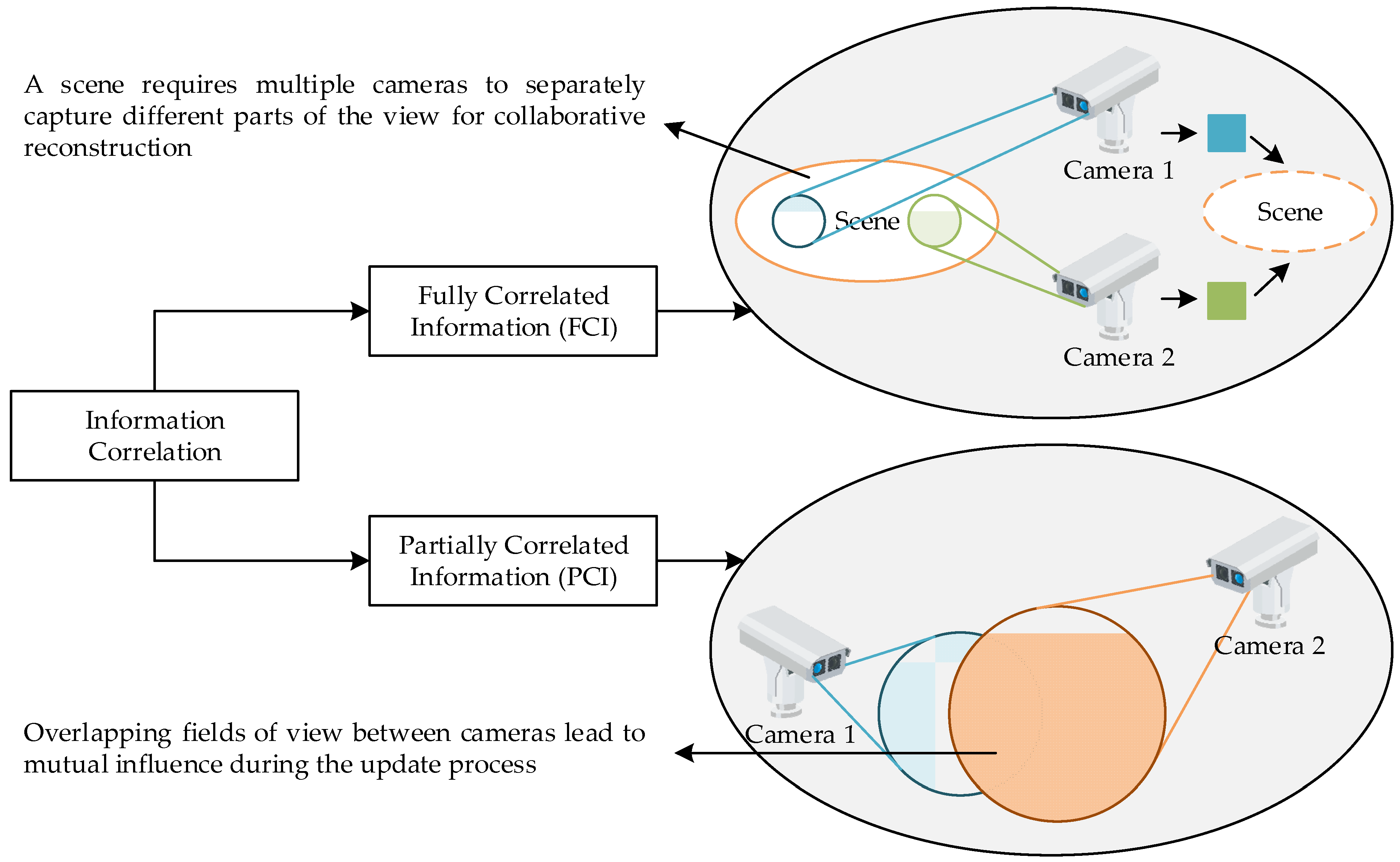
We introduce a novel correlation-aware update model by incorporating an asymmetric correlation matrix to describe the overlapping information among sources. This enables the analysis of spatial redundancy effects on the AoI and quantifies the gain from correlated observations.
(3)
To address practical constraints where correlation structures are unknown, we propose a lightweight least-squares estimation method based on historical AoI data. This estimator provides a scalable and real-time approach to approximating AoI reduction factors in online settings.
(4)
We conduct extensive simulations under heterogeneous IEEE 802.11 [31] Distributed Coordination Function (DCF) conditions, verifying the analytical model and estimator across varying activation rates, network sizes, and correlation levels. The results demonstrate the robustness of the theoretical predictions and highlight the limitations of existing saturation-based approximations in large-scale or correlated environments.
The remainder of the paper is structured as follows. Section 2 describes the network model, correlation model, and SHS-based AoI analysis framework. Section 3 presents the theoretical AoI analysis. Section 4 discusses the simulation results and performance evaluation. Section 5 concludes the paper.

2. System Model

2.1. Network Model

We consider a CSMA network in which N source nodes transmit data packets to a shared base station over a wireless channel. These source nodes represent IoT devices, and their spatial distribution follows a homogeneous Poisson point process (HPPP). The sources are indexed from 1 to N and are uniformly distributed within a unit square centered at the base station. The coverage area of the base station is modeled as a disk with radius R = L / 2 , where L denotes the side length of the square. Accordingly, the node density is defined as λ = N / ( π R 2 ) . We summarize the key notations in Table 1.
In contrast to the conventional arrival–queue–service framework commonly adopted in AoI studies [32], we employ a simplified two-state model for each source, consisting of the idle and active states [33,34]. This abstraction facilitates a tractable analysis of AoI evolution, particularly when incorporating information correlation in later sections.
Specifically, each source transitions from the idle state to the active state according to a Poisson process with rate λ a . Transitioning to the active state indicates that the source is ready to transmit a newly generated data packet. Consistent with the existing literature [35], we adopt the widely used GAW approximation, where a packet is generated and transmitted only when the source successfully completes an exponential backoff and obtains channel access. This assumption avoids the complexity of managing queues and allows for the direct modeling of the AoI at the source level.
During contention, if the source successfully seizes the channel and completes its transmission, it returns to the idle state. In the event of a collision, the data packet is discarded, and the source remains in the active state, initiating a new backoff cycle.
This model retains the essential dynamics of CSMA—namely, random backoff, channel contention, collision, and channel occupancy—while significantly simplifying the AoI analysis. The two-state model used throughout this work can be formally described as follows.
(1)
Idle state: The source is inactive and transitions to the active state at rate λ a .
(2)
Active state: The source prepares to transmit but must undergo a backoff process characterized by an exponential distribution with mean 1 / R i , where R i represents the average backoff attempt rate of source i . Once source i completes backoff and successfully accesses the channel, it begins transmission. The transmission duration follows an exponential distribution with mean 1 / H i , where H i denotes the average transmission rate. If the transmission succeeds, the source returns to the idle state. If a collision occurs, the packet is dropped, and the source remains active to initiate a new backoff.
This abstraction enables the effective analysis of the age dynamics under contention and packet loss, serving as a natural foundation for the relevance-aware AoI framework introduced later. The idle–active source model has also been validated in various real-world scenarios, such as wireless sensor networks and industrial IoT systems, where information timeliness is prioritized over throughput.

2.2. Correlated Sources Model

According to [29], information correlation among sources can be effectively characterized by their geographical proximity and data sampling similarity, which together reflect spatial correlation. In this study, we model such correlation using an undirected graph G = ( N , E ) , where N denotes the set of N sources and E represents the set of edges, capturing pairwise information dependencies. The edge set E can be represented as an N × N matrix: E = [ e 1 , e 2 , , e N ] , where each row vector e n is defined as e n = [ e n 1 , e n 2 , , e n N ] , with E [ 0 , 1 ] N × N . Each matrix entry e i j represents the AoI reduction factor at the base station for source j when source i successfully transmits an update. Intuitively, if sources i and j are geographically close or semantically correlated, the information provided by j can partially substitute that of i , thereby reducing the perceived AoI of i at the base station. In the special case of self-representative updates, we set e i i = 1 for all i N , indicating that a source’s own update fully refreshes its status. However, due to variations in physical locations and sensing modalities, the correlation matrix E is generally asymmetric, i.e., e i j e j i for some i , j N .
For example, as illustrated in Figure 2, the sensing region of source 1 overlaps by 50% with that of source 2, whereas the sensing region of source 2 overlaps by 30% with that of source 1. Consequently, the corresponding AoI reduction factors are given by e 21 = 0.5 and e 12 = 0.3 , respectively. This example highlights the asymmetric nature of the correlation matrix E , stemming from the directional and heterogeneous relevance between sources.

2.3. SHS Model for AoI Analysis

The AoI quantifies the time elapsed since the most recently generated and received update at the monitor. Suppose that update i is generated at time u i ( t ) and subsequently transmitted to the monitor. At any given time t , the monitor observes the freshest received update, and its corresponding AoI is defined as t u i ( t ) . The AoI increases linearly with time until a new update is received, at which point it resets. The average AoI is defined as the time average of the instantaneous age function Δ ( t ) over a sufficiently long interval τ , as depicted in Figure 3, and is given by Δ τ = 1 τ 0 τ Δ ( t ) , d t . Let the interarrival time and system time of the n -th update be denoted by Y n = t n t n 1 and T n = t n t n , respectively, where t n is the generation time and t n is the reception time. As shown in Figure 3, the area under the AoI curve corresponding to update n is calculated as Q n = 1 2 ( T n + Y n ) 2 1 2 T n 2 , which represents the contribution of update n to the overall age integral. Accordingly, the average AoI over τ can be expressed as the limiting time average of these contributions as τ . The average AoI is
Δ = lim τ Δ τ = E [ Q n ] E [ Y n ] .
For the detailed analytical procedures involved in applying Equation (1) to various queuing systems, please refer to the tutorial in [5]. In complex CSMA systems, traditional graphical methods to compute the average AoI may become cumbersome or inaccurate, especially under scenarios involving information correlation. To address these challenges, we adopt the SHS approach to model and evaluate the average AoI. The SHS framework models the system as a continuous-time Markov chain (CTMC) and incorporates continuous age evolution processes during state transitions, thereby enabling equilibrium-based analysis through joint distributions of states and age variables.
Following the notation in [5], the SHS model is defined using a hybrid process ( q ( t ) , x ( t ) ) , where
(1)
q ( t ) denotes the discrete state of the network at time t , with representing the set of all possible network states; the vector notation q ( t ) is used to express structured state labels;
(2)
x ( t ) = [ x 0 ( t ) , x 1 ( t ) , , x K ( t ) ] is a continuous-valued vector representing the age of different status variables—specifically, x 0 ( t ) denotes the age of the most recently received update at the monitor. For 1 i K , x i ( t ) represents the age of the update stored at position i in the source queue.
The Markov chain can be represented by ( , L ) , where L is the set of state transitions. Each transition l L is associated with a departure state q l and an arrival state q l and occurs at rate λ ( l ) δ q l , q ( t ) . The outgoing and incoming transition sets are defined as
L q = { l L : q l = q } , L q = { l L : q l = q } .
In SHS, the Markov chain component captures the complex interactions of events occurring within the network. In the context of AoI analysis, an essential counterpart is the evolution of the age at the monitor. Specifically, transitions in the discrete state process can trigger updates in the continuous age process. When a transition l occurs, the system moves from the discrete state q l to q l . Simultaneously, if this transition represents the successful delivery of a status update to the monitor, the continuous state x is reset according to x = x A l , where A l is the reset matrix associated with transition l . This reset mechanism is crucial in accurately modeling the age dynamics during state transitions. Between discrete transitions, the continuous state evolves linearly over time. For each discrete state q ( t ) , the continuous evolution is governed by the following differential equation:
x ˙ = b q .
In this differential equation, b q = [ b q 0 , b q 1 , b q 2 , , b q K ] is a binary vector indicating the evolution behavior of each age component in discrete state q . Specifically, b q i = 1 if and only if the corresponding age component x i ( t ) increases at a unit rate while the system is in state q ; otherwise, b q i = 0 , indicating that x i ( t ) remains constant in this state. For instance, since the monitor continuously tracks the staleness of received updates, the first element of this vector always satisfies b q 0 = 1 for all q . To compute the long-term average AoI under the SHS framework, it is necessary to define the following quantities for each discrete state q :
π q ( t ) = E [ δ q , q ( t ) ] = P ( q ( t ) = q ) ,
ν q ( t ) = [ v q 0 ( t ) , v q 1 ( t ) , , v q K ( t ) ] = E [ x ( t ) δ q , q ( t ) ] ,
where π q ( t ) denotes the steady-state probability of the Markov chain being in discrete state q at time t , while ν q ( t ) represents the joint moment between the continuous age process x ( t ) and the discrete state q ( t ) . To guarantee the existence and uniqueness of the steady-state distribution, we assume that the Markov chain q ( t ) is ergodic. This assumption ensures that the system converges to a unique stationary distribution over time. Accordingly, the steady-state probability vector is defined as π ¯ = π ¯ q q , which satisfies the global balance equations
π ¯ q l L q λ ( l ) = l L q λ ( l ) π ¯ q l , q ,
q π ¯ q = 1 .
Further details are provided in [5], which proves that, under ergodicity, the conditional age vector ν q ( t ) satisfies the following balance equation:
ν ¯ q l L q λ ( l ) = b q π ¯ q + l L q λ ( l ) ν ¯ q l A l , q .
Finally, the average AoI at the monitor is given by
Δ = q v ¯ q .
The above results form the foundation for AoI analysis via the SHS approach. These expressions will be used in the following sections to evaluate the average AoI under specific network scenarios.

2.4. Markov Chain

In a CSMA network, our analysis focuses on a designated target source, while the remaining n = N 1 sources are modeled collectively as background sources, each potentially operating with distinct activation rates.
A key modeling approach involves aggregating the collective impact of these background sources into a compact state representation. Specifically, the overall network state at any given time is represented as an ordered pair, where the first element indicates the state of the target source and the second element captures the joint state of the background sources. The complete state space is denoted by and is formally defined as
= { ( I , Q ) , ( A , Q ) , ( C , Q ) , ( I , C ) , ( A , C ) } ,
which enumerates all possible combinations of the form (target state, background state). The interpretation of each state is as follows.
(1)
State ( I , Q ) : The target source is idle, while at least one background source is actively contending for the channel. The label “Q” generically denotes the presence of background contention without identifying specific sources. In practice, multiple background sources may contend simultaneously. Thus, even if one background source succeeds in transmission, the system may remain in the “Q” state due to ongoing contention from others.
(2)
State ( A , Q ) : The target source is active and has initiated its exponential backoff process. Simultaneously, background sources are also contending for channel access.
(3)
State ( C , Q ) : The target source has completed its backoff, successfully acquired the channel, and has started transmitting. Background contention continues during this period.
(4)
State ( I , C ) : The target source is idle, and a background source has completed its backoff and is currently transmitting.
(5)
State ( A , C ) : The target source is active, but a background source has already acquired the channel and is transmitting.
It is important to note that, due to the carrier-sensing mechanism inherent in CSMA, any ongoing transmission suspends the backoff timers of all other contending sources. As a result, the target source can only complete its backoff and begin transmission if no background source is currently transmitting. Therefore, the state ( C , C ) is invalid. Additionally, the memoryless property of exponential distributions ensures that, after a freeze or collision, the resumed backoff is statistically identical to the original.
Figure 4 presents the SHS-based Markov chain model constructed for the system. A state transition occurs whenever one of the following events takes place:
(1)
The target source becomes active with activation rate λ a ;
(2)
Any source—either the target or one of the background sources—successfully acquires the channel for transmission;
(3)
A collision occurs, resulting in a transmission failure;
(4)
A transmission successfully completes, and the transmitting source returns to the idle state.
Figure 4. SHS-based Markov chain for the target node in a CSMA network.
Electronics 14 02688 g004

3. Performance Analysis

3.1. SHS State Transitions and Parameter Computation

In the presence of information correlation, a successful transmission from the target source not only updates its own AoI, but transmissions from other correlated sources can also reduce its AoI. To model this behavior, we adopt the GAW model, following the formulation in [36], to quantify the AoI dynamics throughout the network. Specifically, each time a source completes its backoff, it immediately generates and attempts to transmit a new packet. Let x i ( t ) denote the AoI of source i at time t . If source i successfully transmits a packet to the monitor at time t (i.e., without collision), its AoI is reset to zero. Otherwise, if no transmission occurs or the attempt results in a collision, the AoI is updated by scaling its previous value with a reduction factor α i ( t ) [ 0 , 1 ] , which captures the degree of indirect freshness improvement due to correlated updates from other sources. Thus, the AoI evolution for source i at time t is given by
x i ( t ) = 0 , i f   s o u r c e   i   s u c c e s s f u l l y   t r a n s m i t s , x i ( t ) α i ( t ) , o t h e r w i s e ,
where
α i ( t ) = j T g t ( 1 e j i ) ,
where α i ( t ) denotes the residual AoI factor for source i , capturing the extent to which successful transmissions from other sources at time t contribute to reducing the AoI of source i . Let T g t represent the set of sources that successfully transmit at time t . It is important to note that x ( t ) reflects the AoI state immediately after any such event at time t . Between successful updates, the AoI values increase linearly over time.
For example, consider the scenario illustrated in Figure 2. Suppose that the initial AoI values of source 1 and source 2 at time t are x 1 ( t ) = 10 and x 2 ( t ) = 10 , respectively. If source 1 successfully transmits a packet at time t , then its AoI is reset to zero: x 1 ( t ) = 0 . Meanwhile, the AoI of source 2 is updated using Equation (11) as
x 2 ( t ) = 10 × 1 0.3 = 7 .
This illustrates that the AoI update at source i is influenced not only by its own transmission events but also by successful transmissions from other sources correlated with it.
When the target source is in the idle state ( I ) and a background source is in the active state ( A ) , a successful transmission attempt by a background source j leads to a transition of the channel back to the idle state. At this point, two outcomes are possible.
(1)
Collision: If source j encounters a collision, resulting in a failed transmission, the AoI of the target source i remains unchanged.
(2)
Successful transmission: If source j transmits successfully without collision, then—due to information correlation—the AoI of the target source i is updated. This update is governed by the correlation coefficient e i j , as defined in Section 2.2, and is expressed as
x i ( t ) = x i ( t ) α i ( t ) = x i ( t ) ( 1 e j i ) .
The continuous process in the SHS framework is given by
x ( t ) = [ x ( t ) ] ,
where x ( t ) tracks the AoI as observed at the monitor. When a new update packet is successfully received, the monitor’s AoI x is reset to reflect the freshness of the newly delivered information. Under the GAW model, packets are generated instantaneously upon the initiation of transmission. Given that this work focuses on CSMA networks where queuing delays are negligible, the transmission delay is assumed to be zero. Consequently, each successful update immediately resets the AoI to zero. This behavior is mathematically modeled as
x = x A l .
Under this condition, the corresponding component in the age vector x is reset to zero. All transition events within the SHS model are summarized in Table 2. As illustrated in Figure 4, each directed edge from state q ( t ) to q l is associated with a transition rate λ ( l ) . When such a transition occurs, the age vector is updated according to x A l , where A l denotes the reset matrix governing the age evolution. The vector v q A l captures the joint distribution between the age process x ( t ) and the discrete Markov state q ( t ) and is essential in evaluating the average AoI via Equation (8).
(1)
l = 1 : When the target source is in the idle state ( I ) and background sources are in the contention state ( Q ) , the target becomes active at rate λ a . No packet is generated or transmitted at this point, so the monitor’s AoI remains unchanged: x = x .
(2)
l = 2 : The target source is in the active state ( A ) while background sources remain in contention ( Q ) . Upon completing its backoff, the target transitions to the transmission state ( C ) . Since the update has not yet reached the monitor, the AoI remains unchanged: x = x .
(3)
l = 3 : The target is transmitting in state ( C ) , but a collision occurs with probability p (where 1 / H 1 is the mean transmission time), resulting in a dropped packet. The source remains in ( C ) , and the AoI is not updated: x = x .
(4)
l = 4 : The target is in state ( C ) , and its transmission completes successfully with probability 1 p . The source returns to the idle state ( I ) , and the monitor receives a new update, leading to an AoI reset: x = 0 .
(5)
l = 5 : The target remains idle ( I ) while one of the N background sources successfully acquires the channel at rate R 2 . Since the update is not from the target, the AoI remains unchanged: x = x .
(6)
l = 7 : During transmission by the target source, it undergoes an activation event, transitioning from ( I ) to ( A ) at rate λ a . As this event does not result in a successful update, the AoI is unaffected: x = x .
(7)
l = 8 : A background source completes its transmission. Since the target did not transmit, no AoI update occurs: x = x .
(8)
l = 6 , 9 : The target source is in an idle ( I ) or active ( A ) state, and a background transmission results in collision and failure. The channel becomes free again, and the target state remains unchanged. No AoI update occurs: x = x .
(9)
l = 10 , 11 : The target source is in an idle ( I ) or active ( A ) state, and a background source successfully transmits a packet. Although the target’s state does not change, the monitor receives correlated information due to information relevance. Therefore, the AoI of the target is partially updated according to the correlation model
x = α ¯ x ,
where α ¯ represents the average residual factor of the target source’s AoI when updates are successfully transmitted by other sources. This parameter serves to simplify the AoI model for long-term average analysis by eliminating the need to explicitly track each successful transmission from individual background sources. Based on the system parameters—namely, the activation rate λ of each source and the correlation coefficient e j i between background source j and the target source i —the average residual factor α ¯ i for the target source can be expressed as
α ¯ i = j = 1 j i n u j e j i ,
where u j denotes the proportion of the total transmission activity attributed to source j and is defined as
u j = λ j k = 1 k i n λ k .
In practical decentralized scenarios where the monitor lacks knowledge of individual sources’ activation rates or the inter-source correlation coefficients, the value of α ¯ i cannot be directly computed. To address this limitation, we propose an estimation method based on the observed AoI dynamics at the monitor. Drawing inspiration from the approach in [29], we employ a least-squares estimation technique. Let D g = x i ( t + 1 ) 1 and D f = x i ( t ) 1 , where t = 1 , 2 , , T . The estimated value of α ¯ i is then given by
α ^ i = k = 1 t ( D f k D ¯ f ) ( D g k D ¯ g ) k = 1 t ( D f k D ¯ f ) 2 ,
where
D ¯ f = k = 1 t ( x i ( k ) 1 ) t , D ¯ g = k = 2 t + 1 ( x i ( k ) 1 ) t ,
The detailed computation procedure is presented in Algorithm 1.
Algorithm   1 :   Least-Squares   Estimation   of   Correlation   Coefficient   α ^ i
Input : AoI   observations   of   source   i :   x i ( 1 ) , x i ( 2 ) , , x i ( T + 1 ) ; Output: Estimated   correlation   coefficient   α ^ i ; 1     Initialize   t = 1 , 2 , , T ;       Compute   difference   sequences: 2       D g = x i ( t + 1 ) 1 ,   for   t = 1 , 2 , , T ,      D f = x i ( t ) 1 ,   for   t = 1 , 2 , , T ; 3     Compute   sample   means   using   Equation   ( 21 ) ; 4     Apply   least-squares   estimation   ( Equation   ( 20 ) ) ; 5     Return   α ^ i .
In Table 2, p denotes the collision probability, which can be computed using either fixed-point approximations or MAC-layer analytical methods, as outlined in [25]. Returning to the SHS framework, and under the simplifying assumption that queuing delays are negligible, the continuous process x evolves according to the following first-order differential equation for the case k = 1 :
x ˙ = b q ,
where
b q = 1 .
This indicates that, in any discrete state q , the AoI increases linearly over time. Specifically, the age variable x evolves at a unit rate during the continuous phase between discrete transitions.

3.2. Average AoI Calculation

To compute the average AoI using Equation (8), we first solve for the steady-state distribution of the CTMC, as defined by Equations (6) and (7). The resulting steady-state vector is denoted by π ¯ = π ¯ q q . Equation (6) can then be reformulated in matrix notation as π ¯ D = B ¯ , where
D =   diag λ a + R 2 , R 1 + R 2 , H 1 , λ a + H 2 , H 2 .
The form of matrix B is given as
B = 0 λ a 0 R 2 0 0 0 R 1 0 R 2 1 p H 1 p H 1 0 0 0 H 2 0 0 0 λ a 0 H 2 0 0 0 .
We can now obtain the system’s steady-state probability distribution. Then, using Equation (8), we compute the steady-state age vector:
ν ¯ = ν ¯ ( I , Q ) ν ¯ ( A , Q ) ν ¯ ( C , Q ) ν ¯ ( I , C ) ν ¯ ( A , C ) = v ¯ ( I , Q ) v ¯ ( A , Q ) v ¯ ( C , Q ) v ¯ ( I , C ) v ¯ ( A , C ) .
Specifically, for the state q = ( I , Q ) , Equation (8) yields the following linear balance equation:
( λ a + R 2 ) v ¯ ( I , Q ) = 1 π ( I , Q ) + ( 1 p ) H 1 0 +           p H 2 v ¯ ( I , C ) + ( 1 p ) H 2 α ¯ v ¯ ( I , C ) .
Similarly, the corresponding equations for other states are
( R 1 + R 2 ) v ¯ ( A , Q ) = 1 π ( A , Q ) + λ a v ¯ ( I , Q ) + p H 1 v ¯ ( C , Q )         + p H 2 v ¯ ( A , C ) + ( 1 p ) H 2 α ¯ v ¯ ( A , C ) ,
H 1 v ¯ ( C , Q ) = 1 π ( C , Q ) + R 1 v ¯ ( A , Q ) ,
( H 2 + λ a ) v ¯ ( I , C ) = 1 π ( I , C ) + R 2 v ¯ ( I , Q ) ,
H 2 v ¯ ( A , C ) = 1 π ( A , C ) + λ a v ¯ ( O , C ) + R 2 v ¯ ( A , Q ) .
By solving the full set of equations based on (8), we can obtain the steady-state AoI components: v ¯ ( I , Q ) , v ¯ ( A , Q ) , v ¯ ( C , Q ) , v ¯ ( I , C ) , and v ¯ ( A , C ) . Finally, the average AoI at the monitor is given by
Δ = q v ¯ q = v ¯ ( I , Q ) + v ¯ ( A , Q ) + v ¯ ( C , Q ) + v ¯ ( I , C ) + v ¯ ( A , C ) .

4. Simulation Results

4.1. Simulation Settings

To maintain general applicability, we consider a Wi-Fi network operating under the IEEE 802.11 DCF, which employs a contention-based MAC protocol. The detailed simulation parameters are summarized in Table 3. In this setting, each node generates traffic according to a randomly assigned activation rate, sampled from the distribution defined in Section 2.1. Each successful transmission conveys a single data packet. The average AoI under each configuration is computed by averaging the results over 2000 independent simulation runs, each with a duration of 300 s. To eliminate transient effects, the initial 10% of samples in each run are discarded as a warm-up period. The simulations are conducted under a heterogeneous high-contention environment, where the activation rate (i.e., traffic intensity) of each background source is independently and uniformly drawn from the interval 50 , 500 .
In the simulation, the information correlation matrix E = [ e i j ] is employed to quantify the spatial information correlation among source nodes. Consistent with the modeling approach presented in Section 2.1, source nodes are randomly deployed over a two-dimensional area according to a HPPP, thereby capturing the inherent spatial randomness in node placement. To characterize the impact of the inter-node distance on the likelihood of information sharing, the off-diagonal entries of the matrix E are computed using the following expression:
e i j = ω i exp k L i , j , i j ,
where L i , j represents the Euclidean distance between nodes i and j ; ω i ( 0 , 1 ) denotes the importance weight of node j from the perspective of node i , reflecting the perceived informational value of node j to node i ; and k is a tunable parameter controlling the strength of spatial information correlation. A smaller value of k leads to a slower decay in the correlation with distance, indicating that even geographically distant nodes may exhibit non-negligible correlations. In contrast, a larger k enforces stronger spatial locality. Due to the heterogeneity of importance weights ω i and the spatial randomness in node distribution, the resulting matrix E is generally asymmetric, thereby more accurately capturing the asymmetry in the information contribution and update effectiveness among sources.

4.2. Simulation Results and Analysis

Figure 5 illustrates the variation in the average AoI at the target source as a function of the activation rate, under different network scales, with the number of sources set to N = 2 , 6 , 10 , 15 . The figure compares the theoretical predictions, simulation results, and estimated values. The theoretical values are computed using Equation (18) with the true correlation matrix, while the estimated values are obtained from historical AoI observations via the parameter estimation method described in Equation (20). The simulation results are obtained empirically from system execution. The correlation strength parameter is fixed at k = 1 , corresponding to weak information correlation, which limits indirect AoI improvement from correlated updates.
As the network size increases—particularly in the high-activation-rate region (e.g., above 50 activations per second)—noticeable discrepancies between the theoretical and simulated results begin to emerge, especially for N = 15 . While the overall trends of all three curves remain consistent, the deviations become more evident as N increases.
This discrepancy primarily arises due to two modeling limitations. First, the SHS model incorporates collision effects by relying on approximations derived from saturated MAC analysis. In large-scale networks, however, the proportion of non-saturated sources grows under heterogeneous activation conditions, thereby introducing structural bias into the theoretical prediction. Second, the SHS model abstracts the contention and backoff procedures as memoryless exponential processes. In practice, the contention behavior in CSMA networks—especially under high traffic—is governed by discrete binary exponential backoff (BEB), which exhibits non-memoryless dynamics. These features are not fully captured by the SHS framework, leading to decreased theoretical accuracy under heavy loads.
Additionally, the estimation curve also shows growing deviations as N increases. This is because the inferred correlation matrix becomes less reliable under large-scale settings. Although the correlation strength is weak ( k = 1 ), the structure of the matrix may exhibit asymmetry and localized imbalance, thereby degrading the effectiveness of the least-squares estimation in Equation (20). Notably, this effect is amplified by statistical variance and insufficient historical data coverage under heterogeneous source activation.
In contrast to [25], which assumes a queue length of one and FCFS transmission, our simulation adopts the GAW model, where each source transmits only the freshest update. Even in the absence of correlation, the AoI values in our simulation appear slightly lower, since no queuing delay is introduced. This is more reflective of latency-sensitive IoT applications.
Figure 6 shows the average AoI at the target source as a function of the activation rate, with the total number of nodes set to N = 2 , 6 , 10 , 15 and the correlation strength parameter fixed at k = 0.4 , representing a moderate level of information correlation. Compared to the weakly correlated scenario ( k = 1 ), the AoI under k = 0.4 is consistently lower across all activation rates. This demonstrates that even partial correlation among sources can significantly improve information freshness by enabling indirect updates and reducing redundancy. Furthermore, the AoI achieves its minimum at a lower activation rate when k = 0.4 , indicating that correlation accelerates AoI reduction and allows efficient freshness maintenance at lower transmission frequencies.
Discrepancies between the theoretical and simulated AoI become more noticeable as the network size N or the activation rate increases. These deviations are mainly due to the simplifying assumptions of the SHS model—such as saturation-based MAC approximations and memoryless contention abstraction—which become less accurate under heterogeneous traffic conditions.
The estimation method also shows a slight increase in error under this setting. Moderate correlation increases the structural asymmetry of the correlation matrix, making the estimation more sensitive to variability in the observed AoI. The limited observation horizon and traffic imbalance across nodes further amplify the estimation inaccuracies.
Despite these deviations, the theoretical model captures the essential trends and confirms the value of exploiting information correlation. Compared to [25], where correlation is absent, our framework achieves greater AoI reduction across all rates. Notably, the AoI minimum occurs at a smaller activation rate, validating the efficacy of incorporating correlation for delay-sensitive and energy-efficient IoT communications.
Figure 7 explores the impact of spatial information correlation on the AoI by comparing two network sizes ( n = 6 and n = 15 ) under a fixed activation rate of 50, which approximates the optimal operating point for the minimization of the AoI. The simulation results reveal that as the correlation strength increases, the target node’s average AoI significantly decreases. This demonstrates that stronger spatial correlation allows the target to benefit from updates sent by other sources, reducing its own transmission burden and improving the timeliness.
The theoretical and simulation results are largely consistent across different correlation levels, with discrepancies diminishing in high-correlation regimes. This is because stronger correlation stabilizes system behavior, making the SHS model’s approximations more accurate. The estimation method performs reliably under both low and high correlation strengths yet shows a systematic upward bias in the intermediate regime (e.g., k 0.4 to 0.6 ). This can be attributed to the increasing uncertainty in correlation inference when partial dependencies dominate. In such cases, the asymmetry or irregularity in the correlation matrix may cause temporal fluctuations in indirect update benefits, reducing the reliability of the historical AoI samples used to estimate the residual reduction factor. Consequently, the estimator may overpredict the correlation gain, resulting in the observed estimation bias. In our simulations, the estimation is performed using the complete historical data sample, and its accuracy is influenced by both the amount of past data and the structural symmetry of the correlation matrix. Specifically, limited historical samples and strong asymmetry in the matrix can amplify the fluctuations in the observed AoI, thereby compromising the estimation reliability and leading to larger deviations in the computed average AoI. Despite these limitations in unknown settings, the estimator remains a practical and reasonably accurate tool for trend analysis, especially when full correlation information is unavailable.

5. Conclusions

This paper presents an SHS-based analytical framework to evaluate the AoI in CSMA networks with correlated sources. By jointly modeling contention, backoff, collisions, and information correlation, we derive a closed-form expression for the average AoI of a target source. Additionally, we propose a practical estimation method for scenarios where the correlation matrix is partially known or unknown. The simulation results validate the accuracy of the proposed model across a wide range of network sizes and correlation strengths. The findings demonstrate that leveraging information correlation can significantly enhance the timeliness performance without increasing the transmission load, which is especially beneficial for dense or energy-constrained IoT environments. The estimation method also proves effective for decentralized implementations where global correlation knowledge is unavailable.
Future work can further enhance the realism and applicability of this framework by
(1)
Incorporating discrete backoff distributions and binary exponential backoff (BEB) mechanisms as specified in IEEE 802.11 standards;
(2)
Modeling physical layer effects such as signal attenuation, fading, interference, and signal-to-noise ratio (SNR) variations, to better simulate practical wireless environments;
(3)
Accounting for heterogeneous modulation and coding schemes (MCS) and mechanisms such as automatic retransmissions (ARQ) and prioritized channel access (e.g., EDCA);
(4)
Extending the model to multi-AP scenarios and inter-network interference in high-density urban deployments;
(5)
Performing a quantitative analysis of the energy consumption, especially under low-power regimes;
(6)
Scaling up the simulations to investigate extreme-density deployments (e.g., thousands of nodes), which are typical in smart cities or industrial monitoring;
(7)
Exploring mobility-induced dynamics and time-varying correlation structures to evaluate the robustness of the framework under realistic, dynamic IoT settings.

Author Contributions

Conceptualization, L.L. and S.Z.; methodology, L.L. and S.Z.; validation, L.L. and S.Z.; formal analysis, L.L. and S.Z.; investigation, L.L. and S.Z.; writing—original draft preparation, L.L. and S.Z.; writing—review and editing, L.L. and S.Z. All authors have read and agreed to the published version of the manuscript.

Funding

This work was supported in part by the Natural Science Foundation of Jiangsu Province (Grant No. BK20241778) and the National Natural Science Foundation of China (No. U2340221).

Data Availability Statement

The original contributions presented in this study are included in the article. Further inquiries can be directed to the corresponding author.

Conflicts of Interest

The authors declare no conflicts of interest.

References

  1. Ke, Y.; Ni, Z.; Zhang, D.; Miao, X.; Leow, C.Y.; Wang, S.; Pan, G.; An, J. Information Freshness in Multi-Hop Satellite IoT Systems. IEEE Trans. Mob. Comput. 2025, 24, 6014–6029. [Google Scholar] [CrossRef]
  2. Liu, Y.; Deng, Q.; Zeng, Z.; Liu, A.; Li, Z. A Hybrid Optimization Framework for Age of Information Minimization in UAV-assisted MCS. IEEE Trans. Serv. Comput. 2025, 18, 527–542. [Google Scholar] [CrossRef]
  3. Reddy, Y.A.K.; Venkatesh, T. Age of Information Analysis for Queueing Systems with Proactive Obsolete Packet Management: Multi-Hop, Multi-Source, and Priority Mechanisms. IEEE Trans. Netw. Sci. Eng. 2025, 1–13. [Google Scholar] [CrossRef]
  4. Kaul, S.; Yates, R.; Gruteser, M. Real-time status: How often should one update? In Proceedings of the 2012 Proceedings IEEE INFOCOM, Orlando, FL, USA, 25–30 March 2012; pp. 2731–2735. [Google Scholar]
  5. Yates, R.D.; Kaul, S.K. The age of information: Real-time status updating by multiple sources. IEEE Trans. Inf. Theory 2018, 65, 1807–1827. [Google Scholar] [CrossRef]
  6. Sun, Y.; Uysal-Biyikoglu, E.; Yates, R.D.; Koksal, C.E.; Shroff, N.B. Update or wait: How to keep your data fresh. IEEE Trans. Inf. Theory 2017, 63, 7492–7508. [Google Scholar] [CrossRef]
  7. Yates, R.D. Lazy is timely: Status updates by an energy harvesting source. In Proceedings of the 2015 IEEE International Symposium on Information Theory (ISIT), Hong Kong, China, 14–19 June 2015; pp. 3008–3012. [Google Scholar]
  8. Kosta, A.; Pappas, N.; Ephremides, A.; Angelakis, V. Age and value of information: Non-linear age case. In Proceedings of the 2017 IEEE International Symposium on Information Theory (ISIT), Aachen, Germany, 25–30 June 2017; pp. 326–330. [Google Scholar]
  9. Zhou, B.; Saad, W. Minimizing age of information in the Internet of Things with non-uniform status packet sizes. In Proceedings of the ICC 2019—2019 IEEE International Conference on Communications (ICC), Shanghai, China, 20–24 May 2019; pp. 1–6. [Google Scholar]
  10. Jiang, Z.; Krishnamachari, B.; Zheng, X.; Zhou, S.; Niu, Z. Timely status update in wireless uplinks: Analytical solutions with asymptotic optimality. IEEE Internet Things J. 2019, 6, 3885–3898. [Google Scholar] [CrossRef]
  11. Kadota, I.; Sinha, A.; Modiano, E. Optimizing age of information in wireless networks with throughput constraints. In Proceedings of the IEEE INFOCOM 2018—IEEE Conference on Computer Communications, Honolulu, HI, USA, 16–19 April 2018; pp. 1844–1852. [Google Scholar]
  12. Kadota, I.; Sinha, A.; Modiano, E. Scheduling algorithms for optimizing age of information in wireless networks with throughput constraints. IEEE/ACM Trans. Netw. 2019, 27, 1359–1372. [Google Scholar] [CrossRef]
  13. Kadota, I.; Modiano, E. Age of Information in Random Access Networks with Stochastic Arrivals. In Proceedings of the IEEE INFOCOM 2021—IEEE Conference on Computer Communications, Vancouver, BC, Canada, 10–13 May 2021; pp. 1–10. [Google Scholar]
  14. Chen, X.; Gatsis, K.; Hassani, H.; Bidokhti, S.S. Age of Information in Random Access Channels. In Proceedings of the 2020 IEEE International Symposium on Information Theory (ISIT), Los Angeles, CA, USA, 21–26 June 2020; pp. 1770–1775. [Google Scholar]
  15. Yavascan, O.T.; Uysal, E. Analysis of Slotted ALOHA With an Age Threshold. IEEE J. Sel. Areas Commun. 2021, 39, 1456–1470. [Google Scholar] [CrossRef]
  16. Yates, R.D.; Kaul, S.K. Status updates over unreliable multiaccess channels. In Proceedings of the 2017 IEEE International Symposium on Information Theory (ISIT), Aachen, Germany, 25–30 June 2017; pp. 331–335. [Google Scholar]
  17. Jones, N.; Modiano, E. Minimizing Age of Information in Spatially Distributed Random Access Wireless Networks. In Proceedings of the IEEE INFOCOM 2023—IEEE Conference on Computer Communications, New York, NY, USA, 17–20 May 2023; pp. 1–10. [Google Scholar]
  18. Kaul, S.; Gruteser, M.; Rai, V.; Kenney, J. Minimizing age of information in vehicular networks. In Proceedings of the 2011 8th Annual IEEE Communications Society Conference on Sensor, Mesh and Ad Hoc Communications and Networks, Salt Lake City, UT, USA, 27–30 June 2011; pp. 350–358. [Google Scholar]
  19. Tripathi, V.; Jones, N.; Modiano, E. Fresh-CSMA: A distributed protocol for minimizing age of information. J. Commun. Netw. 2023, 25, 556–569. [Google Scholar] [CrossRef]
  20. Pan, H.; Chan, T.T.; Li, J.; Leung, V.C.M. Age of Information With Collision-Resolution Random Access. IEEE Trans. Veh. Technol. 2022, 71, 11295–11300. [Google Scholar] [CrossRef]
  21. Jiang, Z.; Liu, Y.; Hribar, J.; DaSilva, L.A.; Zhou, S.; Niu, Z. SMART: Situationally-Aware Multi-Agent Reinforcement Learning-Based Transmissions. IEEE Trans. Cogn. Commun. Netw. 2021, 7, 1430–1443. [Google Scholar] [CrossRef]
  22. Wang, S.; Cheng, Y.; Cai, L.X.; Cao, X. Minimizing the Age of Information for Monitoring over a WiFi Network. In Proceedings of the GLOBECOM 2022—2022 IEEE Global Communications Conference, Rio de Janeiro, Brazil, 4–8 December 2022; pp. 383–388. [Google Scholar]
  23. Wang, S.; Cheng, Y. A Deep Learning Assisted Approach for Minimizing the Age of Information in a WiFi Network. In Proceedings of the 2022 IEEE 19th International Conference on Mobile Ad Hoc and Smart Systems (MASS), Denver, CO, USA, 19–23 October 2022; pp. 58–66. [Google Scholar]
  24. Maatouk, A.; Assaad, M.; Ephremides, A. On the Age of Information in a CSMA Environment. IEEE/ACM Trans. Netw. 2020, 28, 818–831. [Google Scholar] [CrossRef]
  25. Wang, S.; Ajayi, O.T.; Cheng, Y. An Analytical Approach for Minimizing the Age of Information in a Practical CSMA Network. In Proceedings of the IEEE INFOCOM 2024—IEEE Conference on Computer Communications, Vancouver, BC, Canada, 20–23 May 2024; pp. 1721–1730. [Google Scholar]
  26. He, Q.; Dan, G.; Fodor, V. Joint Assignment and Scheduling for Minimizing Age of Correlated Information. IEEE-ACM Trans. Netw. 2019, 27, 1887–1900. [Google Scholar] [CrossRef]
  27. Zhou, B.; Saad, W. On the Age of Information in Internet of Things Systems with Correlated Devices. In Proceedings of the GLOBECOM 2020—2020 IEEE Global Communications Conference, Taipei, Taiwan, 7–11 December 2020; pp. 1–6. [Google Scholar]
  28. Hoang, L.M.; Doncel, J.; Assaad, M. Age-Oriented Scheduling of Correlated Sources in Multi-server System. In Proceedings of the 2021 17th International Symposium on Wireless Communication Systems (ISWCS), Berlin, Germany, 6–9 September 2021; pp. 1–6. [Google Scholar]
  29. Tong, J.W.; Fu, L.Q.; Han, Z. Age-of-Information Oriented Scheduling for Multichannel IoT Systems With Correlated Sources. IEEE Trans. Wirel. Commun. 2022, 21, 9775–9790. [Google Scholar] [CrossRef]
  30. Tripathi, V.; Modiano, E. Optimizing age of information with correlated sources. In Proceedings of the Twenty-Third International Symposium on Theory, Algorithmic Foundations, and Protocol Design for Mobile Networks and Mobile Computing, Seoul, Republic of Korea, 17–20 October 2022; pp. 41–50. [Google Scholar]
  31. IEEE Std 802.11-1997; IEEE Standard for Wireless LAN Medium Access Control (MAC) and Physical Layer (PHY) Specifications. IEEE: Piscataway, NJ, USA, 1997. [CrossRef]
  32. Akar, N.; Ulukus, S. Age of information in a single-source generate-at-will dual-server status update system. IEEE Trans. Commun. 2025, 1. [Google Scholar] [CrossRef]
  33. Wang, M.; Dong, Y. Broadcast age of information in CSMA/CA based wireless networks. In Proceedings of the 2019 15th International Wireless Communications & Mobile Computing Conference (IWCMC), Tangier, Morocco, 24–28 June 2019; pp. 1102–1107. [Google Scholar]
  34. Gamgam, E.O.; Akar, N.; Ulukus, S. Cyclic scheduling for age of information minimization with generate at will status updates. In Proceedings of the 2024 58th Annual Conference on Information Sciences and Systems (CISS), Princeton, NJ, USA, 13–15 March 2024; pp. 1–6. [Google Scholar]
  35. Bhat, R.V.; Vaze, R.; Motani, M. Throughput maximization with an average age of information constraint in fading channels. IEEE Trans. Wirel. Commun. 2020, 20, 481–494. [Google Scholar] [CrossRef]
  36. Kadota, I.; Sinha, A.; Uysal-Biyikoglu, E.; Singh, R.; Modiano, E. Scheduling policies for minimizing age of information in broadcast wireless networks. IEEE/ACM Trans. Netw. 2018, 26, 2637–2650. [Google Scholar] [CrossRef]
Figure 1. Illustrative comparison of fully and partially correlated information models in multi-camera systems.
Electronics 14 02688 g001
Figure 2. A simple example illustrating the overlapping sensing regions between two sources.
Electronics 14 02688 g002
Figure 3. AoI evolution over time.
Electronics 14 02688 g003
Figure 5. Average AoI of the target source versus the activation rate under different numbers of sources, with correlation strength parameter k = 1 (no correlated sources). The solid curve (Sim.) represents the simulation results using the actual system behavior; the dashed curve (Theo.) denotes the theoretical results computed based on the true correlation matrix; the triangle markers (Est.) show the values estimated from observed AoI data using a least-squares fitting method with an estimated correlation matrix.
Electronics 14 02688 g005
Figure 6. Average AoI of the target source versus the activation rate under different numbers of sources, with correlation strength parameter k = 0.4 (presence of correlated sources). The solid curve (Sim.) represents the simulation results using the actual system behavior; the dashed curve (Theo.) denotes the theoretical results computed based on the true correlation matrix; the triangle markers (Est.) show the values estimated from observed AoI data using a least-squares fitting method with an estimated correlation matrix.
Electronics 14 02688 g006
Figure 7. Average AoI of the target source versus correlation strength parameter k , under a fixed activation rate of 50. The solid curve (Sim.) represents the simulation results using the actual system behavior; the dashed curve (Theo.) denotes the theoretical results computed based on the true correlation matrix; the triangle markers (Est.) show the values estimated from observed AoI data using a least-squares fitting method with an estimated correlation matrix.
Electronics 14 02688 g007
Table 1. Notation table.
NotationDescription
N Total number of sources in the network
λ Node density in the network
λ a Activation rate of a source
R i Average backoff rate of source i
H i Average transmission rate of source i
E Correlation matrix
e i j AoI reduction factor at the base station for source j when source i successfully transmits an update
q l Discrete state of the network
x Continuous state of the network
π q ( t ) Steady-state probability of the Markov chain being in discrete state q at time t
n Number of background sources
I Denotes the idle state of the source
A Denotes the active state of the source
C Denotes the state of occupying the channel
Q Denotes the contention state of background sources
α i ( t ) Residual AoI factor for source i at time t
T g t Set of sources that successfully transmit at time t
x ( t ) AoI observed at the monitor at time t
λ ( l ) Transition rate from state q ( t ) to q l
A l Reset matrix governing the age evolution
ν q ( t ) Correlation between the age process x ( t ) and the discrete Markov state q ( t )
α ¯ Average residual factor
α ^ Estimated value of α ¯
p Collision probability
Table 2. SHS state transition table.
l q q l λ l x A l ν q A l
1 I , Q A , Q λ a x   v I , Q
2 A , Q C , Q R 1 x   v A , Q
3 C , Q A , Q p H 1 x   v C , Q
4 C , Q I , Q 1 p H 1 0 0
5 I , Q I , C R 2 x   v I , Q
6 I , C I , Q p H 2 x   v I , C
7 I , C A , C λ a x   v I , C
8 A , Q A , C R 2 x   v A , Q
9 A , C A , Q p H 2 x   v A , C
10 I , C I , Q 1 p H 2 α ¯ x   α ¯ v I , C
11 A , C A , Q 1 p H 2 α ¯ x   α ¯ v A , C
Table 3. Simulation parameter settings.
ParameterDefinitionValue
B R d a t a Bit rate for DATA frame11 Mbps
B R ACK Bit rate for ACK frame1 Mbps
B R P Bit rate for PLCP and preamble1 Mbps
T s l o t Slot time20 μs
D I F S Distributed interframe space50 μs
S I F S Short interframe space10 μs
H P H Y PHY header192 bits
H M A C MAC header224 bits
H I P IP header160 bits
S p Packet payload size8000 bits
A C K ACK packet size 112   bits + H P H Y
W 0 Initial contention window size31
B max Maximum backoff stages5
R max Maximum retransmission limit7
L Side length of the base station area40 m
Disclaimer/Publisher’s Note: The statements, opinions and data contained in all publications are solely those of the individual author(s) and contributor(s) and not of MDPI and/or the editor(s). MDPI and/or the editor(s) disclaim responsibility for any injury to people or property resulting from any ideas, methods, instructions or products referred to in the content.

