Abstract
This study introduces a multi-task prediction model, MT-MBLAE, designed to use DNA methylation data from blood to predict the advancement of Alzheimer’s disease. By integrating various modules, including bi-directional long short-term memory (BiLSTM), long short-term memory (LSTM), and RepeatVector, among others, the model encodes DNA methylation profile data, capturing temporal and spatial information from instantaneous DNA methylation spectra data. Leveraging the network properties of BiLSTM and LSTM enables the consideration of both preceding and subsequent information in sequences, facilitating the extraction of richer features and enhancing the model’s comprehension of sequential data. Moreover, the model employs LSTM, time distributed to reconstruct time series DNA methylation profiles. The time-distributed layer applies identical layers at each time step of the sequence, sharing weights and biases uniformly across all time steps. This approach achieves parameter sharing, reduces the model’s parameter count, and ensures consistency in handling time series data. Experimental findings show the excellent performance of the MT-MBLAE model in predicting cognitively normal (CN) to mild cognitive impairment (MCI), and mild cognitive impairment (MCI) to Alzheimer’s disease (AD).
1. Introduction
AD is a neurodegenerative disease of the elderly. It is one of the most common causes of dementia in the elderly. Its characteristics are memory decline, impaired thinking and understanding ability, loss of judgment, decline in daily life skills, and personality and behavior changes. At present, many studies explored the application of artificial intelligence in AD diagnosis through imaging or molecular data, including gene expression [1,2,3,4]. These applications include detecting the progress of AD [5], early diagnosis [6,7,8], and identifying biomarkers [9,10,11,12,13,14].
Because molecular biology data can accurately describe the correlation between phenotype and genotype, many researchers combined machine learning methods with epigenetics [15,16] and spatial multi-omics [17] to assist in the diagnosis of AD. Early researchers confirmed that DNA methylation can be used as an alternative biomarker for the diagnosis of ad [18,19,20,21]. Because genetic biomarkers from peripheral tissues (such as blood) are non-invasive and easy to obtain, with the development of artificial intelligence, it has become a new research direction to predict the progress of individuals in AD through DNA methylation data extracted from peripheral blood [22,23].
Many studies have been conducted to explore the use of DNA methylation data as predictive biomarkers utilized for diagnosing AD. As an illustration, Bahado-Singh and associates used machine learning techniques, such as deep neural networks and random forests, to differentiate between late-onset AD and healthy individuals [24]. Park et al. utilized deep neural networks to differentiate between AD and control groups by combining DNA methylation data with gene expression data [25], which showed that the combining of gene expression and DNA methylation data led to enhanced prediction accuracy. Tan et al. developed an ensemble model comprising logistic regression, gradient boosting, and support vector machines methods, utilizing demographic and MRI data from the Singapore Dementia Epidemiology Study for early detection of cognitive decline [26]. However, these studies were not longitudinal and could not predict different stages of the disease. Nonetheless, computational approaches for forecasting AD progression with longitudinal data on DNA methylation encounter obstacles because the vast number of epigenetic markers create a high-dimensional prediction task, which continues to be a significant challenge in the field of machine learning. Ray et al. diagnosed AD based on significant methylation changes across the genome in circulating free DNA from AD patients; they used various artificial intelligence technologies and markers of endogenous or exogenous CpG methylation in independent test or validation groups, achieving a value of area under the ROC curve (AUC) over 0.9 [27].
In recent years, several researchers developed efficient deep learning methods employing large-scale, longitudinal studies involving high-dimensional data for out-of-sample forecasting of AD diagnosis and progression. Nivedhitha et al. [28] developed a deep learning model for classifying AD built upon DNA methylation profiles, used an early stopping regularized recurrent neural network (EDRNN) and AdaBoost within a 5-fold cross-validation framework to select features. Li et al. used convolutional neural networks (CNN) with structural MRI to categorize the advancement from MCI to AD and extracted non-invasive MRI indicators related to the advancement of AD [29]. Researchers employed recurrent neural networks (RNN) and LSTM networks to forecast the advancement of AD using a mix of features from demographic data, clinical diagnoses, medical history, neuropsychological assessments, imaging indicators, and cerebrospinal fluid (CSF) metrics [30,31,32]. Cui et al. combined a deep learning architecture of CNN and LSTM (CNNLSTM), utilizing structural MRI to forecast AD progression, where the CNN captures spatial features from images at various time points, while the LSTM captures the temporal relationships of features extracted by CNN [33]. Li et al. created two multi-task deep autoencoders, MT-CAE and MT-LSTMAE, derived from convolutional autoencoders and long short-term memory autoencoders, respectively. These models learn compressed feature representations by concurrently minimizing reconstruction errors and optimizing accuracy in prediction [34].
However, there is still scope for improvement in these models regarding learning compressed representations of features from the longitudinal data DNA methylation and enhancing the prediction performance for AD. This paper proposes a multi-task encoding–decoding model, multi-task model with BiLSTM, and an LSTM auto encoder (MT-MBLAE), which effectively integrates modules such as BiLSTM [35], LSTM [36], RepeatVector, and time distribution to encode and decode the DNA methylation profile data, capturing temporal and spatial information from transient DNA methylation spectra. The model can use DNA methylation data to predict two types of tasks: one is CN to MCI, and the other is MCI to AD. Compared with other model methods, the MT-MBLAE model demonstrates excellent performance.
The main contribution of this article lies in the capability of the MT-MBLAE model to capture richer features, thereby enhancing the model’s understanding of sequential data. Compared with other approaches, MT-MBLAE brings the following contributions:
- (i)
- Combining modules, such as BiLSTM, LSTM, etc., effectively encodes DNA methylation profile data, capturing spatial and temporal information from instantaneous DNA methylation spectra.
- (ii)
- Using RepeatVector duplicates the vector obtained from the encoder several times, generating a new sequence. RepeatVector replicates this vector multiple times along the new time dimension, producing a three-dimensional output, which serves as the input for the decoder, thereby connecting the encoder and the decoder.
- (iii)
- By applying the same layer and its parameters at each time step of the sequence through the time-distributed layer, sharing the same weights and biases across all time steps, parameter sharing is achieved, reducing the model’s parameter count while ensuring consistency in handling time series data.
2. Methods
2.1. The Workflow of DNA Methylation Sequencing in Predicting AD
To utilize DNA methylation for predicting AD, the process starts with extracting cell-free DNA from plasma, obtaining DNA methylation data, and sequencing using a next-generation sequencing (NGS) platform. Subsequently, machine learning is applied to the sequenced data, including methylation, copy number variations (CNV), and fragmentation, to identify the presence of AD. The main workflow is illustrated in Figure 1. The DNA methylation sequencing process is represented in Figure 1A, the workflow for the prediction of AD using DNA methylation is depicted in Figure 1B, and the four types of data used in model training are presented in Figure 1C.
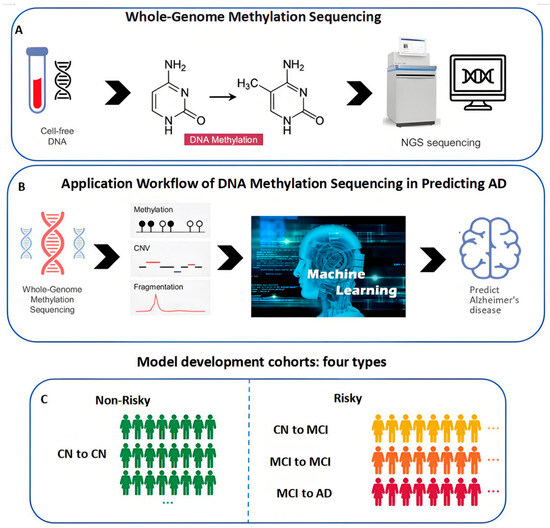
Figure 1.
The workflow of DNA methylation sequencing in predicting AD. (A) The process of creating whole-genome methylation sequencing (WGMS) data. (B) The application workflow of DNA methylation in predicting AD. (C) Model development cohorts: four types.
2.2. Dataset
The datasets are sourced from a cohort of 649 unique individuals taking part in the AD Neuroimaging Initiative (ADNI) ADNIGO and ADNI2. A total of 1905 peripheral blood DNA methylation samples are downloaded from these individuals. These DNA samples have longitudinal data, starting from initial measurement and undergoing visits at intervals of approximately one year or more, with at least four visits, to simulate changes in levels of methylation and depict changes in methylation patterns linked to aging and the advancement of diseases. Derived from clinical data, three types of AD diagnoses were observed: CN, MCI, and AD. Within the cohort of 649 subjects, at baseline, there were 221 individuals classified as CN, 334 individuals with MCI, and 94 individuals with AD. However, at the final visit for each individual, the distribution of AD diagnoses changed to 177 individuals classified as CN, 259 individuals as MCI, and 213 individuals as AD.
From the statistical longitudinal process, the number of diagnoses for each individual is examined. The results reveal that diagnoses remained unchanged for 474 individuals, while 167 individuals had two different diagnoses, and 8 individuals had three different diagnoses. The cohort comprised 167 patients exhibiting two distinct clinical trajectories: 44 progressed from CN to MCI, while 111 advanced from MCI to AD.
Li et al. utilized the Illumina Infinium Human Methylation EPIC BeadChip array to assess each DNA methylation sample, covering approximately 866,000 CpG sites [34]. Samples were randomly allocated using an adjusted incomplete block design to ensure age and gender matching and minimize potential confounders. Beta values for each CpG site, ranging from 0 to 1, were obtained. Subsequently, CpG signals are normalized, batch-corrected, and adjusted for cell type using the ChAMP pipeline. Biological replicates of CpG signals are averaged to obtain normalized methylation profiles for each individual across all CpG sites. Due to uneven visit frequencies for each individual and the possibility of a diagnosis remaining unchanged across multiple visits, the DNA methylation data from the initial and final visits of each participant are utilized as temporal characteristics for the positive dataset. As a result, each individual has two DNA methylation profiles at two time points. Ultimately, the dataset temporal500.h5 is obtained.
In this paper, for the prediction task of CN to MCI, 147 cases of DNA methylation data of CN to CN are used as the negative sample set, and 44 cases of DNA methylation data of CN to MCI are used as the positive sample set. For the prediction task of MCI to AD, 147 cases of DNA methylation data of MCI to MCI are used as the negative sample set, and 111 cases of DNA methylation data MCI to AD are used as the positive sample set.
2.3. Overview of Proposed Deep Learning Model MT-MBLAE
Figure 2 exhibits the overarching structure of the MT-MBLAE model. The MT-MBLAE model structure diagram consists of four core modules: input, encoder, decoder, and prediction modules.

Figure 2.
The structure of proposed MT-MBLAE model.
Input module. The input data include both DNA methylation data and time steps. Here, the data of DNA methylation refer to the quantity at different times, and time steps represent the sequence length, indicating the number of recorded time steps.
Encoder module. This module seeks to acquire compressed feature representations that encapsulate temporal and spatial information from dynamic DNA methylation spectra. It includes both BiLSTM and LSTM modules, where the LSTM in the encoder retains only the data from the last hidden state. The BiLSTM, a distinctive type of RNN, processes sequence data both forward and backward, allowing it to consider both the preceding and following context within the sequence. This capability enhances the model’s understanding of sequence data, capturing richer features and thereby improving model performance.
Decoder module. This module aims to reconstruct the time series of DNA methylation profiles from compressed features. It includes LSTM, which includes all hidden state, time-distributed, and cross-entropy loss [37] modules. The LSTM in the decoder retains the data of all hidden states, and the time-distributed layer applies the same layer and its parameters across each time step in the sequence, sharing weights and biases to reduce the model’s parameters while maintaining consistency in processing time series data. Cross-entropy loss is utilized for calculating loss to guide model training, measuring the disparity between the generated probability distribution and the true target distribution. Through minimizing this loss, the model learns to adjust its parameters to make the generated data closely resemble the real data.
Prediction module. This module includes a fully connected (FC) layer along with a softmax function. The FC layer integrates features from the previous layer, connecting each neuron to all neurons in the preceding layer to capture global relationships among different features. The softmax function converts one or more scores into a probability distribution for making predictions.
2.4. Multi-Task Encoder
The multi-task encoder consists of the following components: BiLSTM and LSTM. It employs a model known as BiLSTM, which is based on LSTM [36], an improved model of the traditional RNN [38].
LSTM manages the flow, update, and forgetting of information ingeniously through the introduction of three control gates comprising input gate, forget gate, and output gate, along with a separate cell state. These mechanisms work together to ensure that the network can maintain important information throughout the sequence transmission while forgetting information that is no longer needed, thereby overcoming the problem of long-distance dependencies.
In the LSTM structure, the input value at time slice t is represented as , and stands for the output of hidden nodes from the preceding unit. The formula for the forget gate can be represented as Formula (1):
The symbol σ signifies sigmoid function. is called the forget gate, it decides , which features to update as , and is a value between [0, 1]. Similarly, and after computing through corresponding neural network layers, the formulas are shown as Equations (2) and (3).
is called input gate, and is used to decide which values to update . The calculation formula for is shown as Equation (4).
represents the output gate, and the output feature matrix of all time slices is obtained by the following Formulas (5) and (6):
Since the BiLSTM comprises two LSTM networks moving in opposite directions, the output of BiLSTM is represented as Formula (7):
The RepeatVector is used to replicate its input vector several times, creating a new sequence. Given a vector of fixed length, RepeatVector repeats this vector several times along a new time dimension, generating a three-dimensional output that serves as the input for the decoder, bridging the encoder and decoder. This makes RepeatVector very useful in transforming non-sequential data into sequential data.
2.5. Multi-Task Decoder
The multi-task decoder consists of LSTM (all state), time-distributed, and cross-entropy loss modules.
LSTM (all state). The hidden states are the outputs at each time step of the sequence, representing the network’s internal representation at each point. By returning all hidden states, an output sequence is generated that mirrors the length of the input sequence, encapsulating the network’s understanding and encoding at each time step. On the other hand, cell states function as a mechanism to convey long-term information across the network. They hold information on long-term dependencies within the sequence, aiding in overcoming the long-term dependency challenges that traditional RNNs encounter.
Time-distributed. The time-distributed layer is used to process outputs from the LSTM hidden layers. The input for the time-distributed layer must be at least a three-dimensional vector, which requires configuring the last LSTM layer to return sequences (for instance, by setting the “return_sequences” parameter to “True”). When using the time-distributed layer wrapped around a dense layer, the aforementioned operation is applied independently to the input at each time step t, as Formula (8):
Here, denotes the input data, W represents the weight matrix, b signifies the bias term, and Activation represents the activation function. For all t = 1,…, time steps, the output at each time step retains its independence while effectively learning parameters through shared weights and biases.
Cross-entropy. The core principle of cross-entropy [37] is the amount of additional information needed when encoding the true distribution based on incorrect or partially matched assumptions (i.e., the model’s predictive distribution). Ideally, if the model’s predictions are completely accurate, the cross-entropy equals the entropy of the true distribution; if there are deviations in the predictions, the cross-entropy increases, with the increase reflecting the degree of inaccuracy.
For a binary classification problem, the expression for the cross-entropy loss function is Formula (9):
Here, N represents the count of samples. stands for the actual label of the i-th sample. denotes the model’s predicted probability that the i-th sample is classified in the positive class, and represents the natural logarithm.
2.6. Prediction Module
The prediction module includes an FC layer and a softmax classifier. The FC layer integrates all features extracted by previous layers (such as convolutional or pooling layers), providing a comprehensive information base for the final decision. In classification tasks, the fully connected layer is often used to output prediction results; for instance, it can map integrated features onto specific categories. The softmax classifier takes the generated feature vector as the input, and after passing through the FC layer, it uses Formula (10) to calculate the score for category k.
represents the overall count of categories, and when c = 2, it handles tasks of binary classification. The softmax function converts neuron outputs into values ranging from [0, 1] and ensures their sum equals 1. Essentially, the output scores for each category are transformed into relative probabilities via Formula (11). Thus, the prediction is made by comparing the predicted probabilities for each category.
2.7. Performance Metrics
Due to the significant differences in the counts of positive and negative samples in this study, this paper combines area under the precision–recall curve (AUPRC) [39] and AUC [39] metrics to evaluate the model, while also using four other indicators for comparison, which are accuracy (ACC), sensitivity (SN), specificity (SP), and Matthews’ correlation coefficient (MCC).
AUPRC is the area under the precision–recall curve (PRC) [39], which focuses particularly on the predictive performance of the positive class (minority class) and is very useful for evaluating imbalanced datasets. The AUPRC represents the average performance of a model across all possible classification thresholds, AUC is defined as the area under the ROC curve. The closer the AUPRC and AUC values are to 1, the better the model’s performance.
Precision as Formula (12):
Recall and AUC as Formulas (13) and (14), respectively:
In this context, TP, FN, TN, and FP correspond to the numbers of true positives, false negatives, true negatives, and false positives, respectively. The equations of ACC, SN, SP, and MCC are expounded below in Formulas (15)–(18).
3. Results
3.1. Experimental Setup
The described methods are benchmarked on two tasks: CN to MCI, and MCI to AD. Experiments utilized the adaptive moment estimation (Adam) [40] gradient descent method to adjust the learning rate, enhancing the efficiency and stability of the training process. To prevent overfitting, dropout techniques are employed during model training. For each prediction task, 15% of the overall samples are allocated as an independent test set, while 85% are utilized for training, with 15% of the training set designated for validation. To reduce the impact of randomness and enhance the reliability of the results, each task is trained independently 10 times, with the final evaluation results being based on the average of these 10 outcomes.
3.2. The Analysis of DNA Methylation Data at a Single Stage
To assess the data characteristics across various transitions—CN to CN, CN to MCI, mild cognitive impairment remaining stable (MCI to MCI), and MCI to AD, it is crucial to regularly monitor changes in DNA methylation. By analyzing DNA methylation data collected at different times, we can evaluate the correlation between patients’ DNA methylation across different periods. DNA methylation data detected in an earlier time period are labeled as Period 1 and used as the x-axis, while data detected in a later period are labeled as Period 2 and used as the y-axis, to plot a scatterplot as shown in Figure 3. This allows for assessing the correlation of DNA methylation data of patients over time.
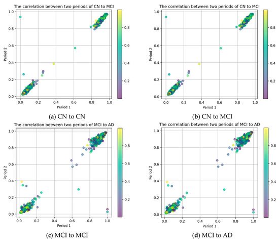
Figure 3.
The relationship between DNA methylation data for a single stage.
For different individual subjects, upon testing DNA methylation data at a single stage, if the DNA methylation data remain linearly correlated, it indicates that the disease progression is slow or temporarily controlled. Conversely, if the correlation between DNA methylation data shows significant changes, it may suggest a transition towards a more severe stage of the disease. From Figure 3, it can be observed that the individual subjects display a linear relationship in their DNA methylation data during the CN to CN (Figure 3a) and MCI to MCI (Figure 3c) stages, whereas some of the DNA methylation data show nonlinear relationships during the CN to MCI (Figure 3b) and MCI to AD (Figure 3d) stages. These results indicate that there are distinctions in the DNA methylation data of subjects at different stages, which can be analyzed to discern the progression of their disease.
3.3. The Analysis of DNA Methylation Data
Treat the DNA methylation data from CN to CN and CN to MCI as one prediction task, predicting the transition from normal to MCI. Consider the DNA methylation data of MCI to MCI and MCI to AD as another prediction task, forecasting the transition from MCI to confirmed AD. In the first task, consider the CN to CN data as negative samples and the CN to MCI data as positive samples; in another task, view the DNA methylation data of from MCI to MCI as negative samples, and from MCI to AD as positive samples. The visualization results of DNA methylation data at two different tasks are represented in Figure 4.

Figure 4.
The visualization analysis of DNA methylation data at different tasks.
From Figure 4a,b, it can see that the positive and negative samples are almost completely overlapping, with no apparent gap. This increases the difficulty for the model to distinguish and extract features from positive and negative samples effectively.
To analyze DNA methylation changes across different populations in the tasks of CN to MCI and MCI to AD, a combined assessment using log2FoldChange [41] and −log10(p-values) is employed. Log2FoldChange denotes the logarithmic ratio of DNA methylation levels between two comparison groups, indicating the magnitude of methylation changes; positive values represent increased methylation, while negative values indicate decreased methylation. −log10(p-values) represents the negative logarithm of p-values obtained from statistical tests to assess the significance of methylation level differences at each site. The higher the value on the vertical axis, the greater the statistical significance.
A threshold is established (p-value < 0.05), typically selecting 0.05 for the p-value. Log2FoldChange is used as the horizontal axis, and −log10(p-values) as the vertical axis, to produce a volcano plot as shown in Figure 4. It is evident that for the CN to MCI task in Figure 5a, the DNA methylation changes in positive and negative samples are well-regulated, with negative samples (CN to CN) concentrated on the left side of the graph and positive samples (CN to MCI) on the right side. A similar pattern is observed for the MCI to AD task in Figure 5b. These results suggest that the changes in DNA methylation levels remain consistent across different stages of AD progression, laying a foundation for subsequent multi-task model predictions.
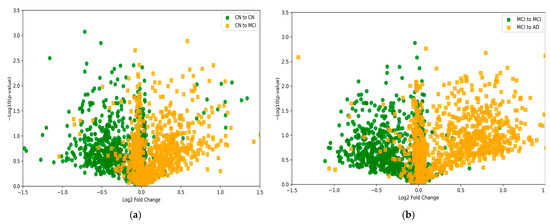
Figure 5.
The DNA methylation changes in adjacent stages of prediction tasks. (a) the task of CN to MCI; (b) the task of MCI to AD.
3.4. The Performance of MT-MBLAE Model
3.4.1. The Relationship Between MT-MBLAE Model Loss and the Number of Epochs
Figure 6 provides a clear visualization of the relationship between the number of epochs and both the training and validation losses of a model. Figure 6a and Figure 6b, respectively, show the changes in model loss over the number of epochs for the prediction tasks CN to MCI and MCI to AD.
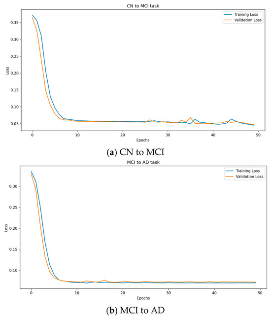
Figure 6.
The relationship between the number of epochs and both the training and validation losses of the MT-MBLAE model.
Initially, both losses are at their highest, peaking at over 0.35 at epoch 1. This indicates that the model begins with limited knowledge about the data and its ability to generalize is not yet developed. As the number of epochs increases, there is a sharp decline in the losses for both the training and validation, suggesting that the model can quickly learn from the training data and refine its predictor. This rapid improvement in loss reduction reflects the capability of the model to adapt its parameters effectively to the underlying patterns in the data. By epoch 20, the decline in losses begins to plateau, indicating that the model started to stabilize. This plateau phase suggests that most of the easy-to-learn patterns have been captured by the model, and additional learning from the training data does not substantially change the performance of the model. When the model reaches epoch 50, both the training and validation losses show minimal changes, with loss as low as 0.05, nearly stabilizing at a constant value. This behavior typically suggests that the model reached its learning capacity, with further epochs providing diminishing returns in terms of loss reduction. At this point, the model is neither significantly overfitting nor underfitting, as the validation loss remains low and stable alongside the training loss.
This analysis points to an optimal stopping point around epoch 50, where extending training further might not yield significant improvements and could risk overfitting if the model starts to learn noise rather than relevant data patterns.
To comprehensively assess the performance of the autoencoder, this paper evaluates the discrepancy between the decoder’s output and the original input data from another perspective by calculating the mean squared error (MSE). As a crucial assessment metric, the lower the MSE value, the closer the autoencoder’s reconstruction is to the original input, indicating better performance.
According to the data presented in Figure 7, whether in the prediction task from CN to MCI or MCI to AD, the model demonstrates a clear trend. As the epoch count during training increases, particularly after reaching 10 epochs, both the MSE of the encoding and the MSE of the validation data significantly decrease, eventually stabilizing at an extremely low level below 0.001. This result highlights the superior performance of the autoencoder in these specific tasks.

Figure 7.
The relationship between the number of epochs and both the encoder MSE and validation encoder MSE of the MT-MBLAE model.
3.4.2. The Impact of Node Quantity on the MT-MBLAE Model in BiLSTM and LSTM
To evaluate the impact of node quantity in the BiLSTM, LSTM, and Dense layers on model performance, this study conducted separate tests on the nodes of each layer. Taking the CN to MCI task as an example, when testing the influence of node quantity in BiLSTM on model performance, the node settings for LSTM and Dense layers were set to typical values, with LSTM set to 256 and Dense set to 64. The node values in BiLSTM ranged from 1 to 512, and the obtained AUC values are shown in the Figure 8. From the Figure 8a, it can be observed that the AUC value reaches its peak when the BiLSTM node value is 177.
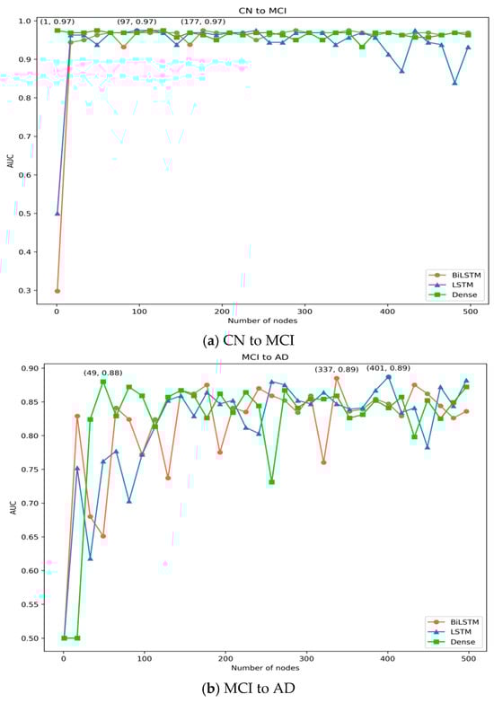
Figure 8.
The impact of BiLSTM, LSTM, and Dense node count on the model’s AUC.
When testing the influence of node quantity in LSTM on model performance, with the BiLSTM node value set to 177 and Dense set to 64, the node values in LSTM ranged from 1 to 512, and the obtained AUC values are shown in Figure 8a. Based on the AUC value, it is apparent that it reaches its maximum when the LSTM node value is 97. Similarly, when testing the influence of node quantity in the Dense layer on model performance, with the BiLSTM node value set to 177 and LSTM set to 97, the node values in the Dense layer ranged from 1 to 512, and the obtained AUC values are shown in the Figure 8. Based on the AUC value, it is apparent that it reaches its maximum when the Dense node value is 1 or 49. Given that a node count of 1 may lead to model instability, the count of Dense nodes is set to 49. Therefore, the count of nodes in the BiLSTM, LSTM, and Dense layers of the CN to MCI task in this study are selected as 177, 97, and 49, respectively.
In the MCI to AD task, the impact of node quantity in the BiLSTM, LSTM, and Dense layers on model performance is illustrated in Figure 8b, yielding similar pattern results as the CN to MCI task. Therefore, the number of nodes in the BiLSTM, LSTM, and Dense layers in this study are selected as 337, 401, and 49, respectively.
3.4.3. The AUC and AUPRC Performance of MT-MBLAE Model
AUC and AUPRC have a higher tolerance for imbalanced data, making these metrics particularly suitable for evaluating model performance on imbalanced datasets. AUC measures the performance of a model across various thresholds, while AUPRC focuses specifically on the predictive performance of the positive class (minority class). MCC and F1 are more sensitive to data imbalance, and MCC is a comprehensive metric that considers TP, FP, TN, and FN, and is very sensitive to data imbalance. The F1 score, being the harmonic mean of precision and recall, can be low for imbalanced data if the model is biased towards predicting the majority class, even if the overall accuracy is high. Therefore, this section uses AUC, ACC, F1, MCC, and AUPRC as evaluation metrics to evaluate the performance of the MT-MBLAE model in predicting MCI to AD and CN to MCI tasks.
The predictive performance of the MT-MBLAE model in predicting the CN to MCI task is shown in Table 1, and the model’s performance in predicting the MCI to AD task is shown in Table 2. It is evident from both tables that the AUC and AUPRC metrics are relatively high, with little variation across the 10 experiments. However, the MCC and F1 metrics show more significant differences across the 10 experiments.

Table 1.
The performance of the MT-MBLAE model in CN to MCI task.
Table 2.
The performance of the MT-MBLAE model in MCI to AD task.
The variability in the Matthews correlation coefficient (MCC) and F1 score in the table can be attributed to the multi-task experiments in this study, where the data subsets used exhibit class imbalance. In the CN to MCI task, the positive samples (CN to MCI) are 44, while the negative samples (CN to CN) are 147. In the MCI to AD task, the positive samples (MCI to AD) are 111, and the negative samples (MCI to MCI) are 147. The uneven number of positive and negative samples causes class imbalance, which makes both the MCC and F1 scores highly sensitive to this imbalance. Therefore, MCC and F1 scores are significantly affected. In terms of the ACC metric, results are almost stable, except in a few experiments. This is related to the use of imbalanced data in this chapter, AUC and AUPRC demonstrate better performance with imbalanced data, indicating that the MT-MBLAE model is effective in forecasting the tasks of CN to MCI and MCI to AD.
3.5. Comparison of MT-MBLAE Model with Other Deep Learning Methods
To evaluate the effectiveness of the MT-MBLAE model with other models, the MT-MBLAE model is compared with MT-CAE [34], MT-LSTMAE [34], and eight other deep learning time prediction methods, making a total of ten methods, see Table 3. These methods are primarily divided into three categories: (i) convolutional neural networks with different counts of convolutional layers (such as CNN1, CNN2); (ii) LSTM and BiLSTM with different counts of LSTM layers (for instance, LSTM1, LSTM2, Bi-LSTM1, and Bi-LSTM2); and (iii) hybrid models combining CNN and LSTM with various counts of LSTM layers (such as CNNLSTM1, CNNLSTM2).
Table 3.
Different deep learning methods.
3.5.1. The Performance of MT-MBLAE Model in CN to MCI Prediction Tasks
This paper uses a boxplot [42] to evaluate the AUC performance of the MT-MBLAE model with other outstanding models, which provides a clear visualization of the dataset’s central tendency and dispersion and can also highlight outliers. A typical boxplot includes the following elements: median, box, whiskers, and outliers.
To mitigate bias in the random stratified sampling process, the procedure is carried out 10 times, and the boxplot of AUC values from the 10 tests is represented in Figure 9.
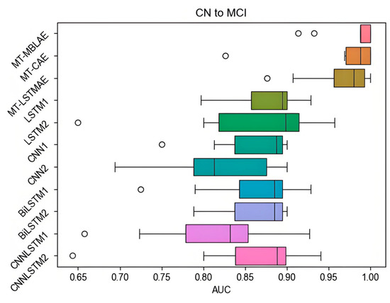
Figure 9.
The AUC value of the MT-MBLAE model in CN to MCI prediction tasks.
Figure 9 illustrates the performance of various models in predicting the progression from CN to MCI. The MT-HBLAE model demonstrates a significantly superior median AUC of 0.9797 (MT-CAE: 0.9715, MT-LSTMAE: 0.9649), with LSTM2, LSTM1, and CNNLSTM2 coming next. The boxplot distribution of the MT-HBLAE model is relatively concentrated with no whiskers, indicating high consistency among the data points, i.e., minimal differences between them. This suggests that the MT-HBLAE model performs well in the CN to MCI task, with AUC prediction performance approaching 1. For other algorithm models, the boxplot distributions are relatively concentrated for MT-LSTMAE and MT-CAE, but the MT-CAE model occasionally has outliers reaching 0.8235, which indicates less stability compared to the MT-HBLAE model. Although the whiskers of the MT-LSTMAE model’s boxplot can reach 1, there is still a gap compared to the MT-MBLAE model, where the boxplot reaches 1. Interestingly, apart from a few models with outliers, circles on the way represent outliers in Figure 9 (the same below in other figures), the performance of the remaining deep learning models is quite consistent, with AUC values all above 0.7. Additionally, the MT-HBLAE model has a smaller boxplot, indicating more concentrated AUC values across multiple experiments, thus demonstrating a more stable performance. These results suggest that the MT-MBLAE model outperforms other methods regarding AUC prediction performance for the CN to MCI prediction task.
In addition to AUC, performance evaluation is also conducted in terms of AUPRC, which is particularly accurate in assessing performance when dealing with imbalanced data. All prediction methods are benchmarked on the two prediction tasks. To reduce the impact of sample randomness and enhance the credibility of the results, the models are executed 10 times, and the AUPRC values from these 10 executions are depicted in a boxplot in Figure 10.
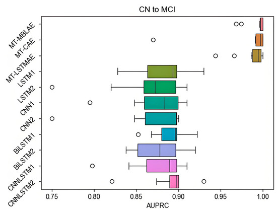
Figure 10.
The AUPRC value of the model in the CN to MCI task.
Figure 10 presents a comparative analysis of AUPRC performance across different deep learning models for predicting the progression from CN to MCI. The MT-HBLAE model demonstrates superior predictive capability with a median AUPRC of 0.997, marginally outperforming other models (MT-LSTMAE: 0.994; MT-CAE: 0.992). The subsequent ranking of model performance reveals CNNLSTM2 (0.8975), LSTM1 (0.8935), CNNLSTM1 (0.8895), CNN2 (0.897), and CNN1 (0.8825), with LSTM2 showing the lowest median performance (0.8725) and a notable outlier (AUPRC = 0.75).
The experimental results, derived from 10 independent trials, indicate that most models achieve AUPRC values within the 0.75–0.95 range, demonstrating reasonable predictive consistency. However, the MT-MBLAE model distinguishes itself through both higher median performance and greater stability, as evidenced by its compact boxplot distribution. These results demonstrate that the MT-MBLAE model outperforms those of other algorithm models.
3.5.2. The Performance of the MT-MBLAE Model in MCI to AD Prediction Task
Figure 11 demonstrates the comparative performance of various deep learning models in predicting the progression from MCI to AD, as measured by AUC values. The MT-MBLAE model emerges as the most effective predictor with a median AUC of 0.895, significantly surpassing other architectures, including BiLSTM2 (0.869), CNNLSTM2 (0.840), and MT-LSTMAE (0.834). These metrics, derived from 10 independent experimental trials, reveal that most models achieve AUC values within the clinically meaningful range of 0.65–0.9, with Bi-LSTM1 being the sole exception at 0.629. These results suggest that the MT-HBLAE model outperforms other methods in terms of AUC prediction performance for the MCI to AD task.

Figure 11.
The AUC value of the MT-MBLAE model in the MCI to AD prediction task.
Figure 12 demonstrates significant variations in AUPRC performance among different models for predicting the conversion from MCI to AD. The MT-HBLAE model substantially outperforms other models with a median AUPRC of 0.9295, which may be attributed to its hybrid bidirectional attention mechanism that enables efficient fusion of multimodal temporal features. Following MT-HBLAE are Bi-LSTM2 (0.913), CNN2 (0.869), and MT-LSTMAE (0.863).

Figure 12.
The AUPRC values of different models in the MCI to AD task.
Notably, the MT-CAE model exhibits an exceptionally low outlier value (AUPRC = 0.525), suggesting potential issues such as vanishing gradients or overfitting in its feature extraction architecture. In contrast, other models consistently achieve AUPRC values between 0.65 and 0.9. These results indicate that the AUPRC values of the MT-MBLAE model outperform those of other algorithm models for the prediction of the MCI to AD task.
The MT-MBLAE model combines the BiLSTM, LSTM, and RepeatVector modules to encode the longitudinal DNA methylation profile data and capture the spatial and temporal information of DNA methylation data. Using the network characteristics of LSTM and BiLSTM, the model can fully consider the previous and subsequent information in the sequence so as to extract more abundant features. In the decoding phase, the combination of LSTM with time distribution and cross entropy loss function enables the model to effectively reconstruct the time series DNA methylation profile data. The design of the time distribution layer enables the same layer and parameters to be shared at each time step of the sequence, thus reducing the number of parameters while ensuring the consistency of the model. Through the effective combination of the encoder and decoder, the mt-mblae model enhances the ability to understand sequence data, and thus shows excellent performance in the multi-task prediction of AD progress.
4. Conclusions
This paper introduces a multi-task prediction model, MT-MBLAE, for predicting the progression of AD from the perspective of deep learning. By effectively combining modules such as BiLSTM, LSTM, RepeatVector, etc., the model encodes DNA methylation profile data, capturing temporal and spatial information from instantaneous DNA methylation spectra. Leveraging the network properties of LSTM and BiLSTM allows for the consideration of both preceding and subsequent information in sequences, enabling the capture of richer features and enhancing the model’s understanding of sequential data. Additionally, the model utilizes LSTM (all hidden state), time-distributed, etc., to reconstruct time series DNA methylation profiles. The time-distributed layer applies the same layer (and its parameters) at each time step of the sequence, sharing the same weights and biases across all time steps, thereby achieving parameter sharing, reducing the model’s parameter count, and ensuring consistency in handling time series data.
This model can predict two types of tasks based on DNA methylation data: CN to MCI and MCI to AD prediction tasks. To mitigate the impact of randomness and enhance result reliability, multiple tests were conducted and compared with other model methods. Experimental results demonstrate the excellent performance of the MT-MBLAE model in predicting the aforementioned tasks. The research in this paper is limited to a single data source, only using longitudinal DNA methylation data, and does not study from a broader perspective, such as multi-omics. In the future, we plan to integrate multi-omics research, conduct further research combined with data of neurodegenerative diseases, such as methylation, transcriptomics, SNPs, and try to conduct external verification.
Author Contributions
Conceptualization, X.Y.; Software, X.Y.; Investigation, R.Z.; Resources, H.L.; Writing—original draft, X.Y.; Writing—review & editing, H.L.; Supervision, R.Z.; Funding acquisition, H.L. and G.Z. All authors have read and agreed to the published version of the manuscript.
Funding
This research was supported by the Education Department of Hainan Province (No. Hnky2024-18), the Hainan Provincial Natural Science Foundation of China (No. 825MS084, No. 823RC488, No. 623RC481, No. 620RC603, No. 721QN0890), the National Natural Science Foundation of China (No. 62262018, No. 62262019), the Haikou Science and Technology Plan Project of China (No. 2022-016), and Hainan Province Graduate Innovation Research Project (No. Qhys2023-408, Qhys2023-407).
Informed Consent Statement
The datasets used in this study are sourced from the AD Neuroimaging Initiative (ADNI) ADNIGO and ADNI2, which involve a cohort of 649 unique individuals. In line with ethical standards in medical research, all participants provided informed consent prior to their inclusion in the study. The ADNI initiative ensures that all patient data is anonymized to maintain privacy and confidentiality, in compliance with relevant data protection laws and regulations such as the Health Insurance Portability and Accountability Act (HIPAA) and the General Data Protection Regulation (GDPR). Additionally, participants were fully informed of the purpose of data collection, including its use in research and model development for AD diagnosis, and were given the option to withdraw from the study at any point without penalty. The ADNI datasets are made available to researchers under strict ethical guidelines to ensure that the privacy and rights of individuals are safeguarded. Furthermore, all research involving these datasets is conducted with transparency, and results are shared in a manner that respects the dignity and autonomy of the participants. Ethical approval for the ADNI study was granted by institutional review boards, ensuring that the research complies with the highest ethical standards in clinical research.
Data Availability Statement
The data supporting this study are openly available at the following URL: https://github.com/lichen-lab/MTAE/blob/main/temporal500.h5 (accessed on 18 April 2025).
Conflicts of Interest
The authors declare no conflict of interest.
References
- Perera, S.; Hewage, K.; Gunarathne, C.; Navarathna, R.; Herath, D.; Ragel, R.G. Detection of novel biomarker genes of Alzheimer’s disease using gene expression data. In Proceedings of the 2020 Moratuwa Engineering Research Conference (MERCon), Moratuwa, Sri Lanka, 28–30 July 2020; IEEE: Piscataway, NJ, USA, 2020. [Google Scholar]
- Lee, T.; Lee, H. Prediction of Alzheimer’s disease using blood gene expression data. Sci. Rep. 2020, 10, 3485. [Google Scholar] [CrossRef]
- Ramaswamy, R.; Kandhasamy, P.; Palaniswamy, S. Feature selection for Alzheimer’s gene expression data using modified binary particle swarm optimization. IETE J. Res. 2023, 69, 9–20. [Google Scholar] [CrossRef]
- Ni, A.; Sethi, A. Alzheimer’s Disease Neuroimaging Initiative. Functional genetic biomarkers of alzheimer’s disease and gene expression from peripheral blood. bioRxiv 2021. [Google Scholar] [CrossRef]
- De la Fuente Garcia, S.; Ritchie, C.W.; Luz, S. Artificial intelligence, speech, and language processing approaches to monitoring Alzheimer’s disease: A systematic review. J. Alzheimer’s Dis. 2020, 78, 1547–1574. [Google Scholar] [CrossRef]
- Thapa, S.; Singh, P.; Jain, D.K.; Bharill, N.; Gupta, A.; Prasad, M. Data-driven approach based on feature selection technique for early diagnosis of Alzheimer’s disease. In Proceedings of the 2020 International Joint Conference on Neural Networks (IJCNN), Glasgow, UK, 19–24 July 2020; IEEE: Piscataway, NJ, USA, 2020. [Google Scholar]
- Murugan, S.; Venkatesan, C.; Sumithra, M.G.; Gao, X.-Z.; Elakkiya, B.; Akila, M.; Manoharan, S. DEMNET: A deep learning model for early diagnosis of Alzheimer diseases and dementia from MR images. IEEE Access 2021, 9, 90319–90329. [Google Scholar] [CrossRef]
- Fisher, C.K.; Smith, A.M.; Walsh, J.R. Machine learning for comprehensive forecasting of Alzheimer’s Disease progression. Sci. Rep. 2019, 9, 13622. [Google Scholar] [CrossRef] [PubMed]
- Modarres, M.H.; Khazaie, V.R.; Ghorbani, M.; Ghoreyshi, A.M.; AkhavanPour, A.; Ebrahimpour, R.; Vahabi, Z.; Kalafatis, C.; Razavi, S.M.K. Early diagnosis of Alzheimer’s dementia with the artificial intelligence-based Integrated Cognitive Assessment: Neuropsychology/computerized neuropsychological assessment. Alzheimer’s Dement. 2020, 16, e042863. [Google Scholar] [CrossRef]
- Esmaeilzadeh, S.; Belivanis, D.I.; Pohl, K.M.; Adeli, E. End-to-end Alzheimer’s disease diagnosis and biomarker identification. In Machine Learning in Medical Imaging. In Proceedings of the 9th International Workshop, MLMI 2018, Held in Conjunction with MICCAI 2018, Granada, Spain, 16 September 2018; Proceedings 9. Springer: Berlin/Heidelberg, Germany, 2018. [Google Scholar]
- Yilmaz, A.; Ustun, I.; Ugur, Z.; Akyol, S.; Hu, W.T.; Fiandaca, M.S.; Mapstone, M.; Federoff, H.; Maddens, M.; Graham, S.F. A community-based study identifying metabolic biomarkers of mild cognitive impairment and Alzheimer’s disease using artificial intelligence and machine learning. J. Alzheimer’s Dis. 2020, 78, 1381–1392. [Google Scholar] [CrossRef]
- Song, M.; Jung, H.; Lee, S.; Kim, D.; Ahn, M. Diagnostic classification and biomarker identification of Alzheimer’s disease with random forest algorithm. Brain Sci. 2021, 11, 453. [Google Scholar] [CrossRef]
- Leuzy, A.; Mattsson-Carlgren, N.; Palmqvist, S.; Janelidze, S.; Dage, J.L.; Hansson, O. Blood-based biomarkers for Alzheimer’s disease. EMBO Mol. Med. 2022, 14, e14408. [Google Scholar] [CrossRef]
- AlMansoori, M.E.; Jemimah, S.; Abuhantash, F.; AlShehhi, A. Predicting early Alzheimer’s with blood biomarkers and clinical features. Sci. Rep. 2024, 14, 6039. [Google Scholar] [CrossRef] [PubMed]
- Sanchez-Mut, J.V.; Gräff, J. Epigenetic alterations in Alzheimer’s disease. Front. Behav. Neurosci. 2015, 9, 347. [Google Scholar] [CrossRef]
- Esposito, M.; Sherr, G.L. Epigenetic modifications in Alzheimer’s neuropathology and therapeutics. Front. Neurosci. 2019, 13, 449570. [Google Scholar] [CrossRef]
- Ma, Y.; Shi, W.; Dong, Y.; Sun, Y.; Jin, Q. Spatial Multi-Omics in Alzheimer’s Disease: A Multi-Dimensional Approach to Understanding Pathology and Progression. Curr. Issues Mol. Biol. 2024, 46, 4968–4990. [Google Scholar] [CrossRef]
- Madrid, A.; Hogan, K.J.; Papale, L.A.; Clark, L.R.; Asthana, S.; Johnson, S.C.; Alisch, R.S. DNA hypomethylation in blood links B3GALT4 and ZADH2 to Alzheimer’s disease. J. Alzheimer’s Dis. 2018, 66, 927–934. [Google Scholar] [CrossRef] [PubMed]
- Kobayashi, N.; Shinagawa, S.; Nagata, T.; Shimada, K.; Shibata, N.; Ohnuma, T.; Kasanuki, K.; Arai, H.; Yamada, H.; Nakayama, K.; et al. Development of biomarkers based on DNA methylation in the NCAPH2/LMF2 promoter region for diagnosis of Alzheimer’s disease and amnesic mild cognitive impairment. PLoS ONE 2016, 11, e0146449. [Google Scholar] [CrossRef]
- Lunnon, K.; Smith, R.; Hannon, E.; De Jager, P.L.; Srivastava, G.; Volta, M.; Troakes, C.; Al-Sarraj, S.; Burrage, J.; Macdonald, R.; et al. Methylomic profiling implicates cortical deregulation of ANK1 in Alzheimer’s disease. Nat. Neurosci. 2014, 17, 1164–1170. [Google Scholar] [CrossRef] [PubMed]
- Comes, A.L.; Czamara, D.; Adorjan, K.; Anderson-Schmidt, H.; Andlauer, T.F.M.; Budde, M.; Gade, K.; Hake, M.; Kalman, J.L.; Papiol, S.; et al. The role of environmental stress and DNA methylation in the longitudinal course of bipolar disorder. Int. J. Bipolar Disord. 2020, 8, 9. [Google Scholar] [CrossRef]
- Wei, X.; Zhang, L.; Zeng, Y. DNA methylation in Alzheimer’s disease: In brain and peripheral blood. Mech. Ageing Dev. 2020, 191, 111319. [Google Scholar] [CrossRef]
- Fransquet, P.D.; Lacaze, P.; Saffery, R.; Phung, J.; Parker, E.; Shah, R.; Murray, A.; Woods, R.L.; Ryan, J. Blood DNA methylation signatures to detect dementia prior to overt clinical symptoms. Alzheimer’s Dementia Diagn. Assess. Dis. Monit. 2020, 12, e12056. [Google Scholar] [CrossRef]
- Bahado-Singh, R.O.; Vishweswaraiah, S.; Aydas, B.; Yilmaz, A.; Metpally, R.P.; Carey, D.J.; Crist, R.C.; Berrettini, W.H.; Wilson, G.D.; Imam, K.; et al. Artificial intelligence and leukocyte epigenomics: Evaluation and prediction of late-onset Alzheimer’s disease. PLoS ONE 2021, 16, e0248375. [Google Scholar] [CrossRef]
- Park, C.; Ha, J.; Park, S. Prediction of Alzheimer’s disease based on deep neural network by integrating gene expression and DNA methylation dataset. Expert. Syst. Appl. 2020, 140, 112873. [Google Scholar] [CrossRef]
- Tan, W.Y.; Hargreaves, C.; Chen, C.; Hilal, S. A machine learning approach for early diagnosis of cognitive impairment using population-based data. J. Alzheimer’s Dis. 2023, 91, 449–461. [Google Scholar] [CrossRef]
- Bahado-Singh, R.O.; Radhakrishna, U.; Gordevičius, J.; Aydas, B.; Yilmaz, A.; Jafar, F.; Imam, K.; Maddens, M.; Challapalli, K.; Metpally, R.P.; et al. Artificial intelligence and circulating cell-free DNA methylation profiling: Mechanism and detection of Alzheimer’s disease. Cells 2022, 11, 1744. [Google Scholar] [CrossRef] [PubMed]
- Mahendran, N.; PM, D.R.V. A deep learning framework with an embedded-based feature selection approach for the early detection of the Alzheimer’s disease. Comput. Biol. Med. 2022, 141, 105056. [Google Scholar] [CrossRef] [PubMed]
- Li, Y.; Haber, A.; Preuss, C.; John, C.; Uyar, A.; Yang, H.S.; Logsdon, B.A.; Philip, V.; Karuturi, R.K.M.; Carter, G.W.; et al. Transfer learning-trained convolutional neural networks identify novel MRI biomarkers of Alzheimer’s disease progression. Alzheimer’s Dement. Diagn. Assess. Dis. Monit. 2021, 13, e12140. [Google Scholar] [CrossRef] [PubMed]
- Wang, T.; Qiu, R.G.; Yu, M. Predictive modeling of the progression of Alzheimer’s disease with recurrent neural networks. Sci. Rep. 2018, 8, 9161. [Google Scholar] [CrossRef]
- Nguyen, M.; He, T.; An, L.; Alexander, D.C.; Feng, J.; Yeo, B.T. Predicting Alzheimer’s disease progression using deep recurrent neural networks. NeuroImage 2020, 222, 117203. [Google Scholar] [CrossRef]
- Lee, G.; Nho, K.; Kang, B.; Sohn, K.-A.; Kim, D. Predicting Alzheimer’s disease progression using multi-modal deep learning approach. Sci. Rep. 2019, 9, 1952. [Google Scholar] [CrossRef]
- Cui, R.; Liu, M.; Alzheimer’s Disease Neuroimaging Initiative. RNN-based longitudinal analysis for diagnosis of Alzheimer’s disease. Comput. Med. Imaging Graph. 2019, 73, 1–10. [Google Scholar] [CrossRef]
- Chen, L.; Saykin, A.J.; Yao, B.; Zhao, F.; Alzheimer’s Disease Neuroimaging Initiative. Multi-task deep autoencoder to predict Alzheimer’s disease progression using temporal DNA methylation data in peripheral blood. Comput. Struct. Biotechnol. J. 2022, 20, 5761–5774. [Google Scholar] [CrossRef]
- Wu, K.; Wu, J.; Feng, L.; Yang, B.; Liang, R.; Yang, S.; Zhao, R. An attention-based CNN-LSTM-BiLSTM model for short-term electric load forecasting in integrated energy system. Int. Trans. Electr. Energy Syst. 2021, 31, e12637. [Google Scholar] [CrossRef]
- Sherstinsky, A. Fundamentals of recurrent neural network (RNN) and long short-term memory (LSTM) network. Phys. D Nonlinear Phenom. 2020, 404, 132306. [Google Scholar] [CrossRef]
- Zhang, Z.; Sabuncu, M.R. Generalized cross entropy loss for training deep neural networks with noisy labels. Adv. Neural Inf. Process. Syst. 2018, 31, 8792–8802. [Google Scholar]
- Li, S.; Li, W.; Cook, C.; Zhu, C.; Gao, Y. Independently recurrent neural network (indrnn): Building a longer and deeper rnn. In Proceedings of the IEEE Conference on Computer Vision and Pattern Recognition, Salt Lake City, UT, USA, 18–23 June 2018. [Google Scholar]
- Ozenne, B.; Subtil, F.; Maucort-Boulch, D. The precision–recall curve overcame the optimism of the receiver operating characteristic curve in rare diseases. J. Clin. Epidemiol. 2015, 68, 855–859. [Google Scholar] [CrossRef] [PubMed]
- Okewu, E.; Misra, S.; Lius, F.S. Parameter tuning using adaptive moment estimation in deep learning neural networks. In Proceedings of the Computational Science and Its Applications–ICCSA 2020: 20th International Conference, Cagliari, Italy, 1–4 July 2020; Proceedings, Part VI 20. Springer: Berlin/Heidelberg, Germany, 2020. [Google Scholar]
- Erhard, F. Estimating pseudocounts and fold changes for digital expression measurements. Bioinformatics 2018, 34, 4054–4063. [Google Scholar] [CrossRef]
- Han, D.; Kwon, S. Application of machine learning method of data-driven deep learning model to predict well production rate in the shale gas reservoirs. Energies 2021, 14, 3629. [Google Scholar] [CrossRef]
Disclaimer/Publisher’s Note: The statements, opinions and data contained in all publications are solely those of the individual author(s) and contributor(s) and not of MDPI and/or the editor(s). MDPI and/or the editor(s) disclaim responsibility for any injury to people or property resulting from any ideas, methods, instructions or products referred to in the content. |
© 2025 by the authors. Licensee MDPI, Basel, Switzerland. This article is an open access article distributed under the terms and conditions of the Creative Commons Attribution (CC BY) license (https://creativecommons.org/licenses/by/4.0/).