A Robust Modeling Analysis of Environmental Factors Influencing the Direct Current, Power, and Voltage of Photovoltaic Systems

Abstract

Solar photovoltaic technology has become a cornerstone of the renewable energy sector over the last 20 years, yet its efficiency remains sensitive to environmental and operational conditions. This study rigorously analyzes how irradiance, temperature, humidity, wind speed, and soiling affect key electrical outputs—Direct current, power, and voltage—of solar panels using advanced robust regression methods: Ridge Regression, Least Absolute Deviation, and M-Estimation. Our results demonstrate that irradiance is the dominant driver of performance, with Ridge Regression coefficients reaching up to 1193 for power. The M-estimation model achieved high predictive accuracy, with R² Scores of 0.989 for current (Mean Squared Error = 0.0399) and 0.991 for power (Mean Squared Error ≈ 10,445), indicating strong model reliability. voltage prediction was more challenging but still robust (R² = 0.836, Mean Squared Error = 49.63). Negative impacts from ambient temperature and humidity were consistently observed across models, while wind speed exhibited a beneficial effect by enhancing cooling and thus improving current and power outputs. Soiling was also identified as a critical factor, significantly reducing power and voltage generation. These findings provide quantifiable evidence of how environmental variables shape solar photovoltaic performance and underscore the importance of environmental monitoring and maintenance strategies to optimize energy yield in operational solar power systems.

1. Introduction

Currently, the importance of solar photovoltaic (PV) technology has become absolutely clear in supporting countries’ need for clean electrical energy. Recently, the growth and spread of the construction of solar stations in countries around the world have been observed for providing clean electricity in urban and rural areas, overcoming many obstacles in providing electrical energy, especially in developing countries. In addition, PV systems are largely evaluated as clean, inexpensive energy providers, and the level and quality of their production/performance are primarily taken into account.

In addition, it is known that the amount of electricity or energy generated by PV systems is fundamentally affected by a number of environmental or external factors affecting the PV systems and their production. For the purpose of improving the performance of PV systems, increasing their production, and protecting them from the factors of extinction and damage, which increases their operational life, the main variables or parameters that affect PV systems should be studied, analyzed, and modeled, i.e., those factors that directly affect the production of the PV systems and their operational life. Among these parameters or variables are temperature, humidity, wind speed, amount of light, amount of dust, altitude, and atmospheric pressure, where these parameters/variables reduce the production and efficiency of PV systems.

The relationship between PV systems and economic sustainability is increasingly recognized as essential for long-term energy strategies. As countries and regions aim to transition to cleaner energy sources, the integration of PV systems offers a viable path toward economic sustainability. Solar power, as a renewable resource, provides an affordable and reliable alternative to traditional fossil fuels, thereby reducing energy costs in the long run. The widespread adoption of PV systems not only generates employment in the renewable energy sector but also stimulates economic growth through the development of green technologies and industries. Additionally, as solar panel production becomes more cost-efficient and installation processes improve, the economic barriers to widespread PV systems adoption continue to lower. This reduces the overall cost of electricity production, making it more accessible, particularly in remote or developing areas. Moreover, investing in PV systems contributes to reducing the economic risks associated with fossil fuel price volatility, fostering energy security, and promoting a sustainable future for global economies.

The global demand for renewable energy is growing at an unprecedented rate, with solar energy emerging as one of the most viable alternatives to conventional fossil fuels. As the efficiency of PV systems continues to improve, understanding the environmental and operational factors that influence solar power generation has become increasingly critical. Despite significant advances in PV technology, the performance of solar panels is still heavily dependent on a range of environmental variables such as solar irradiance, ambient temperature, humidity, wind speed, and panel soiling. These factors introduce significant variability in power generation, which presents both challenges and opportunities for optimizing solar energy production.

While the relationship between solar irradiance and panel output is well documented, the influence of other environmental variables, including temperature, humidity, and wind speed, is more complex and less well understood. Additionally, the effects of soiling—a prevalent issue in regions with low rainfall—can cause significant reductions in the efficiency of solar panels. Understanding how these variables interact and impact the Direct Current (DC), DC power, and DC voltage of solar power systems is essential for optimizing performance and ensuring long-term reliability.

This study aims to contribute to the growing body of literature by employing robust regression models to assess the joint impact of these environmental and operational factors on solar panel performance. Specifically, we focus on the analysis of DC current, DC power, and DC voltage outputs across various conditions. We hypothesize that certain variables—such as irradiance, temperature, and humidity—will have a stronger influence on solar panel performance, while others, such as wind speed and soiling, will act as modifiers of this relationship. By leveraging a robust modeling approach, this study accounts for the inherent variability in environmental data, providing more reliable and generalizable results than traditional linear models.

The efficiency of PV systems is a critical factor in determining the overall effectiveness of solar power generation. PV system efficiency is influenced by a range of variables, including the quality of the solar panels, the angle of installation, and, as discussed, environmental factors such as temperature, irradiance, humidity, and wind speed. Higher efficiency in solar panels leads to the better conversion of sunlight into electricity, maximizing energy production and reducing the need for additional infrastructure or land use. However, maintaining optimal efficiency requires continuous monitoring and adaptation to changing environmental conditions. For example, high temperatures can reduce the efficiency of solar cells, while dust or dirt accumulation on the panel surfaces (soiling) can significantly block sunlight, decreasing the amount of electricity generated. Therefore, improving PV system efficiency involves not only enhancing the technology of the panels themselves but also managing the environmental factors that affect their performance. Ongoing research into advanced materials, coatings, and cleaning technologies, alongside efficient system designs, will be key to improving PV system efficiency and ensuring that solar energy remains a competitive and sustainable energy source for the future.

This research is significant in several ways. First, it offers a comprehensive analysis of the environmental conditions that influence solar power generation in diverse settings. Second, it uses advanced statistical techniques, such as robust regression, to overcome the limitations of the modeling methods, particularly in the presence of outliers or heteroscedasticity. Lastly, the findings can inform practical strategies for improving the efficiency of PV systems, especially in regions with challenging environmental conditions.

2. Related Works

The performance of PV systems is influenced by a wide range of environmental factors, including solar irradiance, temperature, humidity, and wind speed, among others. In addition, there are complex relationships among these factors; these play a critical role in determining the DC current, power output, and voltage in PV systems, affecting their overall efficiency and performance. In order to understand these complex relationships and enhance the predictive modeling of PV system behavior, several studies have investigated the impact of environmental variables on the system’s electrical characteristics. The following table summarizes key studies that have contributed to understanding these influences and offers insights into the methodologies and findings that form the basis of this research.

The studies summarized in

Table 1. Most pertinent works.

	Author (s)	Date	Context of Study	Main Findings
1	Jathar, et al. [1]	2023	This study reviews various environmental factors affecting the performance of PV systems.	- Dust accumulation on the surface of PV modules can significantly reduce energy output (up to 80%).
2	Khaled Hasan, et al. [2]	2022	Comprehensive review of environmental and operational factors affecting the performance of PV systems.	- Solar PV output is highly dependent on solar irradiance; efficiency drops by 0.08% for each degree deviation in irradiance.
3	Olusola, et al. [3]	2025	Comprehensive review of the environmental factors affecting solar PV performance and global trends in solar energy growth.	- Solar Irradiance: the most significant factor influencing PV performance, with the greatest impact near the equator.
4	Ali Al Humairi, et al. [4]	2024	Investigating the effects of soiling on PV system performance using field data from Shams Solar Facility, Oman	- Identified strong positive correlation between DC current and power output, and weak negative correlation between DC current and voltage.
5	Ziqi Yang [5]	2023	Comprehensive analysis of the environmental factors affecting solar cell performance, focusing on dust accumulation, ambient temperature, and humidity.	- Dust Accumulation: dust hinders solar radiation transmission, causes shading, and reduces the PV system’s heat dissipation, significantly lowering efficiency. - Ambient Temperature: high temperatures reduce the operating voltage of the cells, impacting the system’s efficiency. - Shading: shading reduces the amount of sunlight received, further lowering power output. - Humidity: humidity can lead to the formation of water droplets on solar panels, which refracts, reflects, or diffracts sunlight, reducing solar radiation and affecting performance. - Conclusion: The durability and efficiency of solar cells are strongly influenced by environmental factors such as dust, temperature, shading, and humidity. Understanding these factors is critical to enhancing solar cell performance and durability. Research is ongoing to develop more stable and efficient solar cell technologies and improve manufacturing processes. - Future Focus: AI and machine learning will be used to monitor and optimize solar cell performance and mitigate environmental impacts.
6	Yuya Nakamoto, Shogo Eguchi [6]	2024	The study evaluates the impact of seasonal and technical factors on the power generation efficiency of utility-scale PV power plants, using monthly data.	- Generation Efficiency and Performance Ratio (PR): The study evaluates power generation efficiency using the PR and Data Envelopment Analysis (DEA) metrics. Seasonal variations, such as temperature and solar irradiation, significantly impact efficiency, and adjusting the DC/AC ratio (where PV array capacity exceeds inverter capacity) can enhance generation efficiency, particularly during low-insolation periods.
7	Abhishek Kumar Tripathi, et al. [7]	2024	The study explores the use of machine learning (ML) methods for predicting PV panel output, considering fluctuating environmental conditions like temperature, humidity, solar radiation, and dust accumulation.	- ML Models for Prediction: The study compares various ML models for PV power prediction, including Support Vector Machine Regression (SVMR), multivariate regression, and Gaussian regression. Among these, SVMR was found to be the most effective, providing the highest performance with an R2 value of 0.99 and minimal errors. - Impact of Environmental Conditions: Environmental factors such as ambient temperature, humidity, solar radiation, panel temperature, and dust accumulation significantly affect PV panel output. Accurate prediction models are essential for optimizing solar energy systems. - Methodological Comparison: the research differs from other studies by employing a diverse set of models and datasets, considering multiple environmental variables for more robust power prediction. - Techno-Economic and Environmental Assessment: the study not only provides insights into the technical aspects of solar power prediction but also assesses the economic viability and environmental benefits of solar power systems, emphasizing the need for accurate forecasting models to reduce costs and enhance sustainability.
8	David Addae [8]	1982	This thesis critiques traditional industrial growth models for Third World development and explores solar energy as a rural alternative.	- Industrial development based on fossil fuels may not be suitable for Least Developed Countries (LDCs). - Solar energy offers potential benefits for rural development, especially in agriculture.
9	Ramos, et al. [9]	2010	This study presents a MATLAB(https://repqj.com/index.php/repqj/article/view/3450/619-Hernanz accessed on 20 May)-based PV cell/module model and compares it with existing models.	- The developed model accurately represents I-V characteristics using minimal input parameters. - The study highlights the lack of manufacturer-provided resistance values as a limitation.
10	Marcus, et al. [10]	2021	This study proposes integrating solar PV panels with a compressed air system to mitigate losses due to soiling and overheating.	- Compressed air can effectively clean and cool PV panels, increasing their efficiency. - Simulations show that optimal energy gains are achieved by blowing air early in the day or during peak solar radiation. - The system yields an energy Return on Investment (ROI) of 23.8 over two weeks, suggesting it could reduce or eliminate manual cleaning.
11	Subarto, et al. [11]	2013	This paper presents a MATLAB/Simulink-based circuit model to simulate the electrical behavior of a PV array under varying environmental conditions.	- The model incorporates solar irradiance, temperature, shunt resistance, and ideality factor. - A detailed analysis of how these parameters affect output was conducted.
12	Valentin and Zahari [12]	2023	This study models the operation and performance of PV systems for electricity self-consumption under various configurations.	- Accurate hourly load profiles are essential for precise energy calculations. - Battery use significantly increases solar energy self-consumption, with annual unused energy falling below 10%.
13	Yunus, et al. [13]	2018	The study focuses on the mathematical modeling and simulation of a PV cell, module, and array using MATLAB/Simulink, incorporating key parameters and environmental variations.	- The influence of solar irradiation, temperature, and series and shunt resistance on PV behavior was thoroughly analyzed. - The progression from single cell to full array was demonstrated. - Partial shading effects were simulated, confirming the model’s effectiveness in representing real PV behavior.
14	Bekir Cirak [14]	2023	The study develops a circuit-based solar cell model using MATLAB/Simulink, simulating a 5.3 kW PV generator to analyze performance under varying temperature and irradiation.	- The model simulates how changes in temperature and solar irradiance affect voltage and current outputs. - Technical specifications and panel output characteristics were evaluated under standard and varying environmental conditions using graphical outputs.
15	Bharathy and Sumathi [15]	2019	This paper focuses on modeling and simulating the electrical behavior of a solar PV system, emphasizing power electronics and the analysis of key parameters using MATLAB/Simulink.	- Power electronics play a crucial role in energy generation and distribution in PV systems. - The study highlights the future importance of advanced converters and control strategies.
16	Merchant and Embury [16]	2013	This chapter explores the use of radiative transfer simulations in thermal remote sensing of Sea Surface Temperature (SST), focusing on the physics-based modeling of infrared radiance from the ocean surface to the top of the atmosphere.	- Radiative Transfer Models (RTMs) are essential for simulating thermal radiance, accounting for atmospheric gases, aerosols, clouds, and surface properties. - Simulations aid SST retrieval, cloud detection, and uncertainty estimation, all critical for producing reliable climate data records. - Emphasizes the need for physical insight when using RTMs to ensure accurate interpretation and geophysical inversion.
17	Paul Biemer [17]	2009	This chapter examines the measurement errors in survey data and emphasizes the importance of understanding error components in survey responses and data collection methods.	- Measurement errors arise from various sources including poor questionnaire design and data collection methods. - Quantifying measurement error (bias and variance) helps improve survey design and data accuracy. - Emphasizes latent class analysis and Markov latent class analysis for complex error structures. - Understanding measurement errors enhances data analysis validity and interpretation.

highlight the critical role that environmental factors play in determining the performance of PV systems. Key factors such as dust accumulation, solar irradiance, temperature, humidity, and shading are all identified as major influences on PV system efficiency and energy output. This research also emphasizes the importance of accurate predictive models that integrate these environmental variables to optimize PV performance. As machine learning techniques continue to evolve, they offer promising solutions for improving the reliability and efficiency of solar energy systems, particularly in fluctuating conditions. Moving forward, further research into the integration of advanced prediction models, along with the exploration of AI and machine learning technologies, will be essential to overcoming the challenges posed by environmental factors and enhancing the sustainability of solar power systems on a global scale.

3. Research Objectives

The primary objectives of this research are as follows:

• To investigate the influence of environmental and operational factors on the performance of solar power systems, specifically focusing on the DC current, DC power, and DC voltage generated by solar panels.
• To analyze the effects of various environmental predictors (irradiance, temperature, humidity, wind speed, and soiling) on the performance of solar power systems across multiple datasets.
• To identify and quantify the impact of key environmental factors (such as irradiance, temperature, humidity, wind speed, and soiling) on the system’s output, including the effects on DC current, DC power, and DC voltage.
• To assess the role of environmental conditions, particularly wind speed and temperature, in improving or diminishing solar power system efficiency and performance.

4. Materials and Methods

4.1. Problem Selection

The research problem focuses on understanding how various environmental factors influence the performance of PV systems, particularly in terms of DC current, DC power, and DC voltage generated by solar panels. This problem has been selected due to the increasing global emphasis on clean energy development and the need to optimize solar power systems for both economic and environmental benefits. As countries work towards transitioning to renewable energy sources, improving the efficiency of PV systems is essential for reducing costs and maximizing energy output. The aim of this study is to explore the complex interactions between environmental variables—such as irradiance, temperature, humidity, wind speed, and soiling—and the performance of PV systems. By analyzing these factors across multiple datasets using robust regression models, this research aims to provide insights into optimizing solar power generation and system efficiency.

4.2. Data Sources

Data for this study were gathered from the Shams Solar Facility at the German University of Technology in Oman (GUtech), spanning from 9:00 A.M. on 3 April 2021, to 5:05 P.M. on 3 December 2022. The dataset consists of multiple big sets, with each set containing 36,851 data points. The Shams Solar Facility was selected due to its significant role and relevance in the field of renewable energy. A visual representation of the facility is shown in Figure 1.

GUtech’s solar training facility features a diverse range of solar power systems. It includes a ground-mounted system with 20 south-facing modules in portrait orientation, generating about 6 kWp. Additionally, there is a pitched-roof system with 12 south-facing modules in landscape orientation, producing approximately 3900 kWp, as well as two flat-roof systems, each consisting of 12 modules, generating about 3900 kWp. One of the flat-roof systems faces south in portrait orientation, while the other is divided, with half the modules facing east and the other half facing west.

4.3. Environmental Factors Influencing PV Systems

In this study, we focus on the key environmental factors that significantly affect the performance of PV systems, as shown in Figure 1.

As illustrated in Figure 2, the primary environmental variables considered include solar irradiance, which is directly linked to the amount of energy that can be harnessed by the PV panels.

It has been noted from many papers that temperature has a decisive influence on the efficiency and performance of PV cells, as this efficiency is directly affected by temperature. So, the temperature is another critical factor, as high temperatures can reduce the operational efficiency and voltage output of the system. In addition, air pressure and humidity are also essential, as they influence the heat dissipation and the potential for water droplets to obstruct sunlight, thus impacting performance.

Additionally, soiling, or the accumulation of dust on the PV panels, significantly reduces the amount of solar radiation reaching the cells, further decreasing energy production. Wind speed is another key factor, as it can help regulate the temperature of the panels, potentially improving efficiency by providing natural cooling. These environmental factors collectively contribute to the variability in PV system performance, and understanding their impact is crucial for optimizing the efficiency and lifespan of solar power systems.

It is well known that measurement errors occur widely in questionnaire studies due to poorly worded questions that lead to the respondent not understanding them, or the lack of organization and preparation of personal interviews. In addition, the measurement errors are diverse and unavoidable in many experiments [16,17].

However, in this project, the technique of data collection is different than questionnaires, but the measurements error can happen. Also, several actions and procedures were designed and followed in the process of data collection of this project that were designed to minimize the measurement errors [16,17]. These actions and procedures include the following: high-precision advanced sensors were used specifically for such experiments. They were properly prepared and placed in specific fixed locations at the station site. Staff were trained to collect data at fixed, frequent intervals to minimize the impact of human error. A very large size of data was collected from all the environmental factors, thus avoiding these errors. The data were then audited, and no outliers were found to eliminate them.

4.4. Studying Multicollinearity

It is well known that the property of multicollinearity occurs when there is a close relationship (autocorrelation) between the variables. This characteristic greatly affects the precise determination of the effect of each variable on the dependent variable. In addition, the environmental parameters/factors shown in Figure 2 must be free from the autocorrelation in order to model their data. Otherwise, the data of these factors cannot be modeled accurately, and may cause several problems regarding the suitability or goodness of fit of the model, and then in interpreting the results.

In this paper, the multicollinearity is an important factor to study because the performance of PV systems is influenced by several environmental variables that may be correlated. For example, solar irradiance and temperature tend to be positively correlated in many geographic locations, as higher sunlight intensity generally corresponds with higher temperatures. Similarly, factors like humidity and air pressure may also be linked, with high humidity levels often coinciding with lower atmospheric pressure. When these environmental variables are highly correlated, they can cause issues in modeling processes, particularly when trying to assess the individual contribution of each factor to the performance of PV systems.

Addressing multicollinearity in this study is crucial for improving the accuracy and reliability of our predictive models. Where multicollinearity exists, it can lead to inflated standard errors in the coefficients of the estimated model, making it difficult to discern which environmental factor has a true impact on PV performance. This could result in misleading conclusions, where some variables may appear to be less significant than they truly are, or others may seem overly influential. In the context of PV systems, understanding how each environmental factor—such as temperature, irradiance, humidity, and wind speed—individually affects energy output is critical for optimizing performance.

Furthermore, studying multicollinearity helps in identifying potential redundancies in the dataset. By recognizing highly correlated predictors, we can either combine them or remove one from the model, leading to a simpler more interpretable model. This also enhances the stability of the model’s coefficients, making the predictions more robust and generalizable. In practical terms, this is important for the effective deployment of PV systems, as the findings can guide better decision making for system design, maintenance, and operational strategies. Ultimately, accounting for multicollinearity ensures that the results of this study are not only statistically valid but also applicable in real-world scenarios. As PV systems become an increasingly critical component of renewable energy solutions, understanding how environmental factors interact to affect energy output will enable more effective optimization and long-term sustainability of solar energy systems.

5. Modeling Techniques

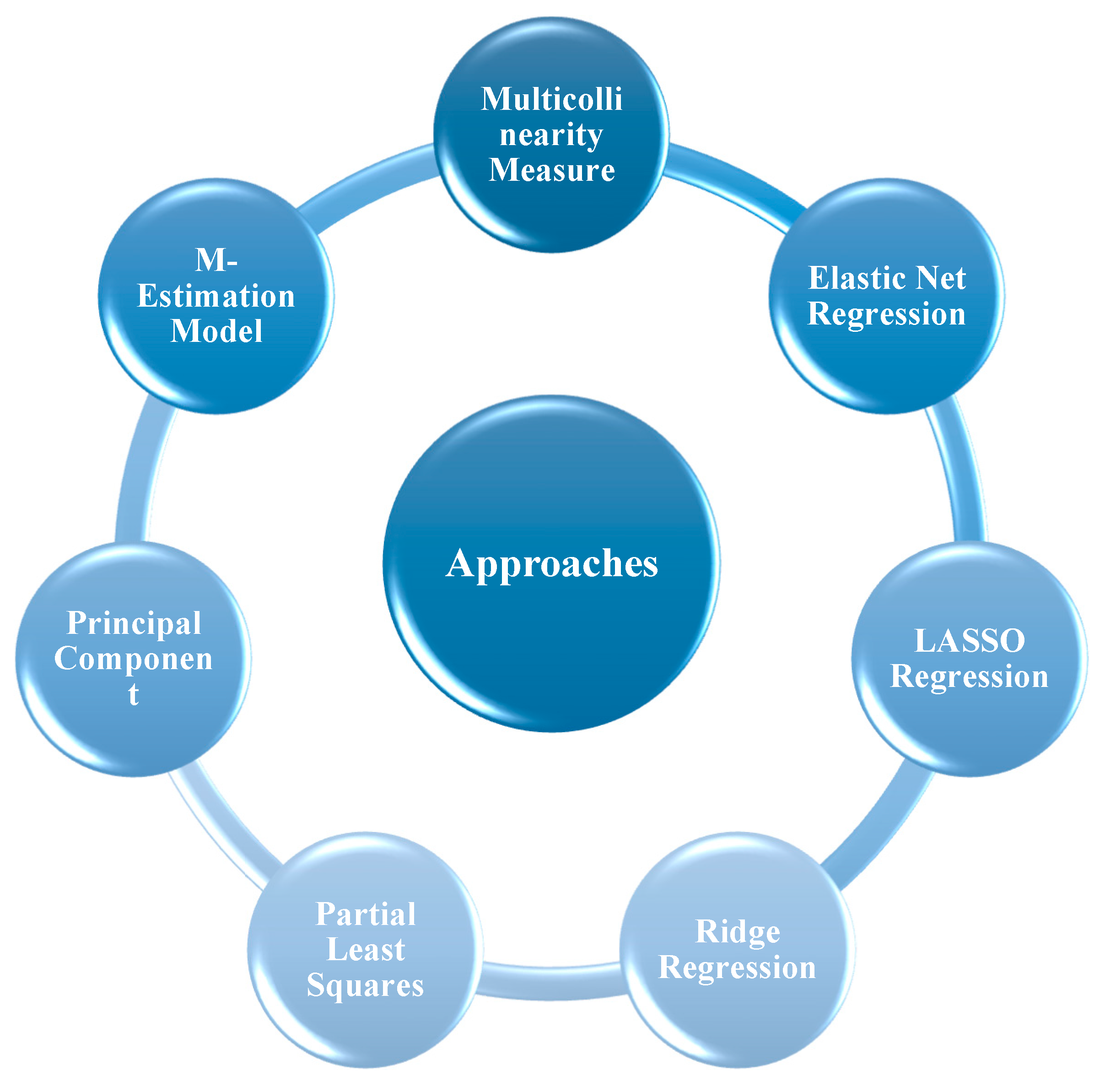
The availability of solar energy makes it a very promising source of electricity, not only for the environment but also for the economy. In addition, its technologies have developed rapidly and sophisticatedly. As a result, solar energy has become a highly effective source of clean energy for various life uses, making its future need urgent and essential and undeniable. Therefore, PV system data modeling is essential for the above reasons.

In this paper, we use six main models as shown in Figure 3.

In this section, we discuss the various techniques and models used in analyzing the environmental factors that influence the performance of photovoltaic (PV) systems. The goal is to apply robust statistical methods to evaluate how different environmental variables, such as solar irradiance, temperature, humidity, and wind speed, impact the energy output of PV systems. Understanding these relationships is essential for optimizing PV system performance. In order to properly model the complex interactions among the predictors, we utilize several advanced regression techniques, including Multicollinearity Measures, Elastic Net Regression, Lasso Regression, and Ridge Regression. Each of these models helps address specific challenges such as correlated predictors, overfitting, and model complexity.

5.1. Multicollinearity Measure

Multicollinearity occurs when two or more predictors in a regression model are highly correlated, which can lead to unreliable estimates of the model parameters. In the context of PV systems, environmental factors like solar irradiance, temperature, and humidity are often correlated, potentially distorting the results of regression analysis. To detect multicollinearity, we use the Variance Inflation Factor (VIF). VIF measures how much the variance of an estimated regression coefficient increases when your predictors are correlated. A VIF value greater than 10 indicates a high multicollinearity problem and suggests that one or more predictors should be removed or combined to improve model reliability.

Where VIF [18,19] uses matrix notations, the calculations may be performed by the following equation:

$$VIF=1/\left(1-R^{2 }\right), and R^{2 }=\left({\underset{¯}{\hat{\beta }}}^{T } {\mathit{Z}}^{T }\underset{\_}{Y}-n{\overline{Y}}^2)/({\underset{¯}{Y}}^T \underset{\_}{Y}-n{\overline{Y}}^2\right)$$

(1)

where $R^{2 }$ is the correlation (COR) square, and the other notations of the above equation are defined in Section 2.

Where R² is the coefficient of determination from a regression model in which the predictor variable is regressed against all other predictors. A higher R² indicates that the predictor variable is highly correlated with other variables, leading to higher VIF values.

5.2. Ridge Regression Model

In order to discuss the models for modeling the data of environmental factors impacting the DC Current, Power, and Voltage of the PV systems, a brief introduction about the Multiple Linear Regression Model (MLRM) should be given.

The Multiple Linear Regression Model (MLRM) is defined by [18,19]

$$\underset{\_}{Y}={\beta }_0+{\beta }_{1 }{Z}_1+{\beta }_{2 }{Z}_2+\dots +{\beta }_r{Z}_{r }+{\mathit{e}}_{\mathit{i}}=\mathit{Z}\underset{\_}{\beta }+\underset{\_}{\epsilon }$$

(2)

where the error term should be satisfied by the following statistical assumptions:

$$E\left(\underset{\_}{\epsilon }\right)=\underset{\_}{0}; and Cov \left(\underset{\_}{\epsilon } {\underset{\_}{\epsilon }}^T \right)={\sigma }^{2}I$$

(3)

The terms of Equation (1) in matrix notations may be defined by the following:

$\underset{\_}{Y}={(Y_1, Y_{2 }, \dots , Y_n )}^T \mathrm{and} \underset{\_}{\epsilon }={({\epsilon }_1, {\epsilon }_{2 }, \dots , {\epsilon }_n )}^T$ (both are n × 1 column vector); $\underset{\_}{\beta }={({\beta }_0, {\beta }_{1 }, \dots , {\beta }_r )}^T$ [is (r + 1) × 1 column vector]; and $\mathit{Z}$ is called by the design matrix [n × (r + 1) matrix] and should be of full rank and is given below, and I is identity matrix of n × n, and

$$Z=\left[\begin{array}{cccc}1& z_{11}& \cdots & z_{1r}\\ & & & \\ 1& z_{21}& & z_{2r}\\ .& .& \ddots & .\\ .& .& & .\\ .& .& & .\\ 1& z_{n1}& \cdots & z_{nr}\end{array}\right]$$

The Ordinary Least Squares (OLS) estimates of the unknown parameters $\underset{\_}{\beta }$ of the model given in Equation (2) above is given by

$$\underset{¯}{\hat{\beta }}={({\mathit{Z}}^{T }\mathit{Z})}^{-\mathbf{1}}{\mathit{Z}}^{T }\underset{\_}{Y},$$

(4)

With residual sum squares given by

$$RSS\left(\underset{\_}{\beta }\right)={{\displaystyle \sum }}_1^n(y_{i }-{\beta }_0-{{\displaystyle \sum }}_{j=1}^r{z}_{ij}{\beta }_{j }{)}^2={(\underset{\_}{Y}-Z\underset{\_}{\beta })}^T\left(\underset{\_}{Y}-Z\underset{\_}{\beta }\right)$$

(5)

It may be mentioned that the above OLS estimators are the Best Linear Unbiased Estimators (BLUEs). However, in several situations the independent random variables ($z_{1 }, z_{2 }, \dots , z_{r }$) or the coefficients $\underset{\_}{\beta }={({\beta }_0, {\beta }_{1 }, \dots , {\beta }_r )}^T$ are highly correlated, i.e., the model is suffering from the multicollinearity; definitely the estimators $\underset{¯}{\hat{\beta }}$ will not be accurate estimators, and will have very high variances, which will reduce the accuracy and the efficiency of the model and its forecasting [20,21,22].

In order to overcome the above limitations, the method of Ridge Regression (RR) is introduced to deal with the problem of multicollinearity of independent variables. The technique of RR is proposed in order to shrink the Relative Risk (RR). The (RR) estimators of the MLRM obtained by incorporating a new quantity denoted by $\mathsf{\lambda } I$ is called the ridge parameter (or penalty of RR). In addition, the RR is based on the diagonal matrix $({\mathit{Z}}^{T }\mathit{Z})$, and is introduced by a new matrix $({\mathit{Z}}^{T }\mathit{Z})$ + $\mathsf{\lambda } \mathit{I}$. The RR estimators are denoted by ${\underset{¯}{\hat{\beta }}}_R$ and are defined by

$${\underset{¯}{\hat{\mathit{\beta }}}}_{\mathit{R}}={({\mathit{Z}}^{T }\mathit{Z}+\mathsf{\lambda } \mathit{I})}^{-\mathbf{1}}{\mathit{Z}}^{T }\underset{\_}{Y}$$

(6)

As mentioned above, the ridge technique will give the estimators ${\underset{¯}{\hat{\mathit{\beta }}}}_{\mathit{R}},$ which minimizes the residual sum of squares (RSS),

$$RSS\left({\underset{\_}{\beta }}_R\right)={(\underset{\_}{Y}-Z\underset{\_}{\beta })}^T\left(\underset{\_}{Y}-Z\underset{\_}{\beta }\right)+\mathsf{\lambda }{\underset{\_}{\beta }}^T\underset{\_}{\beta }$$

(7)

It may be remarked here that the RR estimators ${\underset{¯}{\hat{\beta }}}_R$ given in Equation (5) above have the ability to overcome the problem of multicollinearity in the MLRM model by obtaining shrunken estimated coefficients; therefore, they are characterized by having less variances (Equation (6) above) than the estimators of MLRM.

5.3. Least Absolute Shrinkage and Selection Operator Model

Another approach which has the same aims of RR estimators is called the Least Absolute Shrinkage and Selection Operator (LASSO). The LASSO estimators [21,22,23] are denoted by ${\underset{¯}{\hat{\beta }}}_L$ and given by

$${\underset{¯}{\hat{\beta }}}_L=argmi{n}_{\beta }{{\displaystyle \sum }}_1^n(y_{i }-{\beta }_0-{{\displaystyle \sum }}_{j=1}^r{z}_{ij}{\beta }_{j }{)}^2 subject to {{\displaystyle \sum }}_{j=1}^r{\beta }_{j }\le 1$$

(8)

Also, the LASSO estimators are denoted by ${\underset{¯}{\hat{\beta }}}_L$, which minimize the residual sum of squares,

$$RSS\left({\underset{\_}{\beta }}_L\right)={(\underset{\_}{Y}-Z\underset{\_}{\beta })}^T\left(\underset{\_}{Y}-Z\underset{\_}{\beta }\right)+\mathsf{\lambda } {{\displaystyle \sum }}_1^r\left(\left|{\beta }_j\right|\right)$$

(9)

where “λ is a tuning parameter that controls the shrinkage of the LASSO coefficient with λ ≥ 0” [20,21,22]. It may be worth mentioning that, based on several references, [20,21,22] the LASSO estimator is a worthy competitor to RR estimators.

5.4. Elastic Net Regression Model

It is well known that the LASSO method gives good estimates, behaves well, and exhibits good properties when the independent variables are uncorrelated or not strongly correlated. However, the environmental variables are often highly correlated, leading to poor model performance and weak statistical properties. Thus, a new method is proposed which combines the RR method and the LASSO method, i.e., by incorporating two penalty quantities with the classical residual sum squares. This method is called Elastic Net Regression [20,21,22], and the estimators are denoted by ${\underset{¯}{\hat{\beta }}}_E$ and given by

$${\underset{¯}{\hat{\beta }}}_{LE}=argmi{n}_{\beta }{{\displaystyle \sum }}_1^n{(y_{i }-{\beta }_0-{{\displaystyle \sum }}_{j=1}^r{z}_{ij}{\beta }_{j })}^2 {\mathsf{\lambda }}_1 {{\displaystyle \sum }}_1^r\left(\left|{\beta }_j\right|\right)+{ \mathsf{\lambda }}_2 {{\displaystyle \sum }}_1^r{({\beta }_j )}^2$$

(10)

where $0\le {\mathsf{\lambda }}_1+{ \mathsf{\lambda }}_2 \le 1;$ ${\mathsf{\lambda }}_1 {{\displaystyle \sum }}_1^r\left(\left|{\beta }_j\right|\right)+{\mathsf{\lambda }}_2 {{\displaystyle \sum }}_1^r{({\beta }_j )}^2$ represents the new penalty of Elastic Net approach. The residual sum of squares is

$$RSS\left({\underset{\_}{\beta }}_E\right)={(\underset{\_}{Y}-Z\underset{\_}{\beta })}^T\left(\underset{\_}{Y}-Z\underset{\_}{\beta }\right)+{\mathsf{\lambda }}_1 {{\displaystyle \sum }}_1^r\left(\left|{\beta }_j\right|\right)+{ \mathsf{\lambda }}_2 {{\displaystyle \sum }}_1^r{({\beta }_j )}^2$$

(11)

5.5. Partial Least Squares Model

The Partial Least Squares (PLS) technique is an effective method for obtaining estimates for the parameters of complex multivariate mathematical models and an effective way of reducing the number of model variables, thus retaining only the most important variables based on several criteria. In addition, this method is particularly useful when the independent variables are highly correlated.

This method is based on the MLRM (defined in Equation (2) of Section 2) where the matrix $\mathit{Z}$ is full rank and takes into consideration the related Equations (3)–(5) of the same section. In order to address the problem of multicollinearity of the design matrix $\mathit{Z}$ and to limit the resulting over-variance of model estimators of parameters, the method of Partial Least Squares (PLS) is used. In this method [18,19], the aim is different than the previous methods (Section 2, Section 3 and Section 4), i.e., it is finding $\underset{\_}{\beta }$ with the length $\Vert \underset{\_}{\beta }\Vert =1$ and maximizing

$$COV\left(Z\underset{\_}{\beta }, \underset{\_}{Y}\right)=~COR\left(Z\underset{\_}{\beta }, \underset{\_}{Y}\right)\sqrt[]{VAR\left(Z\underset{\_}{\beta }\right)}$$

(12)

where $COV\left(Z\underset{\_}{\beta }, \underset{\_}{Y}\right)$ is the covariance of $\left(Z\underset{\_}{\beta }, \underset{\_}{Y}\right)$, and $VAR\left(Z\underset{\_}{\beta }\right)$ is the variance of $Z\underset{\_}{\beta }.$

5.6. Principal Component Model

The problem of multicollinearity among matrix variables $\mathit{Z}$ has been addressed in various ways. The principal component (PC) method attempts to reduce the model variables by retaining the important variables that have better predictive performance and so deletes the variables that have a significant negative effect on the final model performance.

Again, the MLRM (defined in Equation (2) of Section 2) is considered where the matrix Z is full rank, and the related Equations (3)–(5) of the same section are considered. In order to address the problem of multicollinearity of the design matrix Z, it is to be understood that this problem is addressed by the PC [18,19] method by transforming the predictor variables (r) into other, smaller set of variables, and then applying the OLS method to the transformed model using the transformed variables, as follows:

Let $q<s$, and define $X_{k }, k=1, 2, \dots , q,$ of $Z_1, Z_2, \dots , Z_{r },$ as

$$X_k={{\displaystyle \sum }}_{j=1}^r\hspace{1em}{\varnothing }_{jk}{Z}_j$$

(13)

where ${\varnothing }_{1k}, {\varnothing }_{2k}, \dots , {\varnothing }_{rk}$ are the new parameters for the transformed model.

The dependent random variable is

$$y_{i }={\theta }_{0 }+{{\displaystyle \sum }}_{k=1}^n{\theta }_k{x}_{ik }, n=1, 2, \dots , n$$

(14)

In the above equation, the dimension of the parameters is reduced from $s+1$ to $q+1$.

After some simplification we get

$${{\displaystyle \sum }}_{k=1}^n{\theta }_k{x}_{ik }={{\displaystyle \sum }}_{k=1}^n{\theta }_k{x}_{ik }\left({{\displaystyle \sum }}_{j=1}^r{\varnothing }_{jk}{z}_{ij }\right)={{\displaystyle \sum }}_{j=1}^r({{\displaystyle \sum }}_{k=1}^n{\theta }_k {\varnothing }_{jk})x_{ik }={{\displaystyle \sum }}_{j=1}^r{\beta }_{j }{z}_{ij}$$

(15)

Equation (15) implies that

$${\beta }_{j }={{\displaystyle \sum }}_{k=1}^q {\theta }_k {\varnothing }_{jk}$$

(16)

5.7. Least Absolute Deviation Model

As is well known, the OLS method for linear regression is ideal when all required regression assumptions are met. However, if some of these assumptions are not met (such as the presence of outliers, the presence of a significant multicollinearity between variables, etc.), the result is that the parameter estimates may be inefficient, and the model may perform poorly. But the method of “Least Absolute Deviation or $L_{1 }$-norm” (LAD) is an alternative to OLS, as the problem of not satisfying the assumptions/requirements does not affect the estimation results and model performance.

The MLRM (defined in Equation (2) of Section 2) is considered where the matrix Z is full rank, and the related Equations (3)–(5) of the same section are considered. In order to address the problem of outliers or multicollinearity of the design matrix Z, the method of $L_{1 }$-norm [22,23,24,25,26] is developed. The method of $L_1$—norm defines the estimators as follows:

$${\underset{¯}{\hat{\beta }}}_{LAD}=argmi{n}_{\beta }{{\displaystyle \sum }}_1^n\left|e_i\right|=argmi{n}_{\beta }{{\displaystyle \sum }}_1^n \left|y_{i }-{\beta }_0-{{\displaystyle \sum }}_{j=1}^r{z}_{ij}{\beta }_{j }\right|$$

(17)

5.8. M-Estimation Model

As we explained in the previous section, linear least squares estimates may not have good statistical properties when the error distribution is not normally distributed and outliers are present. One good solution for this problem is to apply the estimation method called M-method. It differs from the estimation method given in vii as follows:

$${\underset{¯}{\hat{\beta }}}_M=argmi{n}_{\beta }{{\displaystyle \sum }}_1^n\rho \left({\in }_i\left(\beta \right)/\tau \right)$$

(18)

where $\tau$ is “a measure of the scale” and is estimated by

$$\tau =me{d}_i\left|{\tau }_i-\overline{\tau }\right|/0.6745.$$

(19)

where $\overline{\tau }$ denotes the median of the residuals. For iteration t, the estimators ${\underset{¯}{\hat{\beta }}}_M^t$ are given by

$${\underset{¯}{\hat{\beta }}}_M^t={({\mathit{Z}}^{T }{\left({\mathit{W}}^{-\mathbf{1}}\right)}^{\left(\mathit{t}\right)}\mathit{Z})}^{-\mathbf{1}}{\mathit{Z}}^{T }{\left(W^{-1}\right)}^t \underset{\_}{Y} , t=1,2,3, \dots$$

(20)

where ${\left(W^{-1}\right)}^t=diag. \left(w_1^{\left(t\right)}, w_2^{\left(t\right)}, \dots , w_3^{\left(t\right)}\right)$

$$w_i^{\left(t\right)}=\{\begin{array}{c}\phi \left({\displaystyle \frac{y_i-Z_i^t {\beta }^{\left(t\right)} }{{\hat{\tau }}^{\left(t\right)}}}\right) if y_i\ne Z_i^T{\beta }^{\left(t\right)},\\ \\ 1 if y_i=Z_i^T{\beta }^{\left(t\right)},\end{array}$$

(21)

$$\phi \left(z\right)=\{\begin{array}{c}z if \left|z\right|<c, \\ c\left[sgn\left(z\right)\right], if \left|z\right|\le c,\end{array}$$

(22)

and $c\approx 1.345$.

6. Analysis of Multicollinearity

In order to assess the multicollinearity within the model, we computed the VIF for each feature across three dependent variables: DC_CurrentString1_New, DC_PowerString1_New, and DC_VoltageString1_New. In addition, VIF values greater than 10 generally indicate the presence of highly significant multicollinearity, values of VIF between 5 and 10 indicate significant multicollinearity, VIF between 5 and 1 indicate moderate multicollinearity, and the values of VIF = 1 or less indicate that the multicollinearity between the variables does not exist. It is worth noting that the presence of multicollinearity in any data will not lead to inaccurate modeling. This means that the estimated mathematical model for the given data is not trustworthy, and therefore, the results and predictions of such a model are misleading and unreliable. Thus, this feature/property should be studied carefully in the case of modeling the data of a PV system.

In order to summarize the key findings of multicollinearity analyses, the following notations have been developed.

6.1. High Multicollinearity

Several features exhibit extremely high VIF values, suggesting strong multicollinearity and potential redundancy in the data. Notably, they include the following:

IR_S01_RM_Trina_330W13_Irradiance_New (VIF = 227,708.31), Soiling_loss1_New (VIF = 9071,392.07), Soiling_loss2_New (VIF = 9135,051.10), and Soiling_loss_AVG_New (VIF = 4655,248.35) have VIFs that are orders of magnitude higher than the threshold of 10, which could lead to instability in regression models. These features are highly collinear and may contribute to overfitting if included in the model without proper adjustments.

6.2. Infinite

Two features—Air_pressure_relative1_New and Air_pressure_absolute1_New—display infinite VIF values, indicating perfect collinearity with other predictors. This perfect multicollinearity suggests that these variables are redundant and should be excluded from the model so as to prevent issues with model estimation and interpretation.

6.3. Moderate Multicollinearity

Some features exhibit moderate multicollinearity, with VIF values exceeding 10 but not reaching the extreme levels seen in the previously mentioned variables. Key examples include the following:

Si_South_Irradiance_New (VIF = 7040.79), IR_S01_LM_Trina330W14_Irradiance_New (VIF = 53,602.60), and Irradiance_AVG_New (VIF = 149,862.31). These features are highly correlated with other irradiance-related variables, suggesting that careful consideration should be given to their inclusion in the model. Additionally, high VIF values are observed for temperature-related variables such as Si_South_Temperature1_New (VIF = 968.29) and IR_S01_LM_Trina330W14_Temperature1_New (VIF = 2230.07), which may also lead to multicollinearity concerns.

6.4. Low Multicollinearity

Some features exhibit low VIF values, indicating a minimal risk of multicollinearity. These variables include the following:

Ambient_Temperature_New (VIF = 14.03), Wind_speed_New (VIF = 2.31), and Wind_direction_New (VIF = 3.21), which exhibit low VIFs and moderate tolerance values, suggesting that they are less likely to cause issues in the modeling process.

Table 2. Results of low/moderate/high multicollinearity.

Feature	DC_CurrentString1_New (VIF)	DC_PowerString1_New (VIF)	DC_VoltageString1_New (VIF)	Average Tolerance
Si_South_Irradiance_New	7040.79	7040.79	7040.79	1.42 × 10−4
Si_South_Temperature1_New	968.29	968.29	968.29	1.03 × 10−3
IR_S01_LM_Trina330W14_Irradiance_New	53,602.60	53,602.60	53,602.60	1.87 × 10−5
IR_S01_LM_Trina330W14_Temperature1_New	2230.07	2230.07	2230.07	4.48 × 10−4
IR_S01_RM_Trina_330W13_Irradiance_New	227,708.31	227,708.31	227,708.31	4.39 × 10−6
IR_S01_RM_Trina330W13_Temperature1_New	1049.37	1049.37	1049.37	9.53 × 10−4
Irradiance_AVG_New	149,862.31	149,862.31	149,862.31	6.67 × 10−6
Temp_AVG_New	47,168.84	47,168.84	47,168.84	2.12 × 10−5
Air_pressure_relative1_New	∞	∞	∞	0
Air_pressure_absolute1_New	∞	∞	∞	0
Humidity_relative1_New	47.07	47.07	47.07	2.12 × 10−2
Humidity_absolute1_New	33.42	33.42	33.42	2.99 × 10−2
Ambient_Temperature_New	14.03	14.03	14.03	7.13 × 10−2
Wind_speed_New	2.31	2.31	2.31	4.33 × 10−1
Wind_direction_New	3.21	3.21	3.21	3.11 × 10−1
Soiling_ratio1_New	137.29	137.29	137.29	7.28 × 10−3
Soiling_loss1_New	9,071,392.07	9,071,392.07	9,071,392.07	1.10 × 10−8
Soiling_ratio2_New	30.78	30.78	30.78	3.25 × 10−2
Soiling_loss2_New	9,135,051.10	9,135,051.10	9,135,051.10	1.09 × 10−8
Soiling_Ratio_AVG_New	87.08	87.08	87.08	1.15 × 10−2
Soiling_loss_AVG_New	4,655,248.35	4,655,248.35	4,655,248.35	2.15 × 10−7

explores the results of VIF and Average Tolerance and shows that most of the environmental parameters/variables for the three dependent variables are affected by multicollinearity except the variables Wind_speed_New and Wind_direction_New, i.e., the proposed techniques in Section 4 are useful for this situation.

In the following sections, the Elastic Net Regression model, Lasso Regression model, the Partial Least Squares Regression model, and Ridge Regression model are discussed.

7. Modeling Results of Elastic Net Regression

Elastic Net Regression is a powerful modeling technique that combines both Ridge (L2 regularization) and Lasso (L1 regularization) methods. It is particularly useful when dealing with high-dimensional data, as it handles multicollinearity and performs feature selection. The Elastic Net approach shrinks the coefficients of less-important features while preserving significant ones. In this analysis, Elastic Net was applied to three different dependent variables to evaluate its predictive performance and feature importance.

7.1. DC Current

For the model with DC_CurrentString1_New as the dependent variable, the Mean Squared Error (MSE) of the test set was 0.6745, indicating a relatively good model fit. This suggests that the model accurately predicts the target variable, with minimal error.

The Elastic Net coefficients are as follows in

Table 3. Elastic Net coefficients for DC current.

Feature	Coefficient	Feature	Coefficient
Si_South_Irradiance_New	0.2212	Ambient_Temperature_New	0
Si_South_Temperature1_New	0.0676	Wind_speed_New	0.0362
IR_S01_LM_Trina330W14_Irradiance_New	0.1721	Wind_direction_New	−0.0362
IR_S01_LM_Trina330W14_Temperature1_New	0	Soiling_ratio1_New	0.0372
IR_S01_RM_Trina_330W13_Irradiance_New	0.2052	Soiling_loss1_New	−0.0371
IR_S01_RM_Trina330W13_Temperature1_New	0	Soiling_ratio2_New	0.0370
SMP11_BM1_51_Irradiance_New	0.2466	Soiling_loss2_New	−0.0370
Irradiance_AVG_New	0.2000	Soiling_Ratio_AVG_New	0.0369
Temp_AVG_New	0.0289	Soiling_loss_AVG_New	−0.0369
Air_pressure_relative1_New	0	Si_South_Irradiance_New	0.2212
Air_pressure_absolute1_New	0	Humidity_absolute1_New	0
Humidity_relative1_New	0

:

For the model with DC_CurrentString1_New as the dependent variable, the Mean Squared Error (MSE) of the test set was 0.6745, suggesting that the model performs well with a relatively good fit. This low MSE indicates that the model is able to predict the DC current with minimal error, providing reliable estimates based on the input features. The accuracy of the model reflects the significant role that key environmental variables play in predicting the target variable, which is the current output from the solar panels.

The Elastic Net coefficients reveal important insights into which features contribute most to the prediction of DC_CurrentString1_New. Among these, irradiance-related features stand out as the most influential. For example, Si_South_Irradiance_New has a coefficient of 0.2212, and SMP11_BM1_51_Irradiance_New has a coefficient of 0.2466, both showing positive relationships with the DC current. These results are consistent with the expectation that the amount of sunlight (irradiance) directly impacts the current generated by solar panels. As irradiance increases, the solar panels produce more power, which in turn increases the current output. The high coefficients associated with these features emphasize the importance of irradiance in predicting the current.

Similarly, other irradiance features, such as IR_S01_LM_Trina330W14_Irradiance_New (coefficient 0.1721) and Irradiance_AVG_New (coefficient 0.2000), also have positive coefficients, reinforcing the idea that higher levels of irradiance lead to higher current generation. These findings suggest that the model is highly responsive to irradiance values, as they provide a direct indication of how much sunlight the panels are exposed to at any given time.

The soiling-related features also have a notable impact on the DC current prediction. Soiling_ratio1_New and Soiling_loss1_New have coefficients of 0.0372 and −0.0371, respectively, indicating that the amount of soiling and the corresponding loss in energy generation affect the current output. Soiling, which refers to the accumulation of dirt and debris on the surface of the solar panels, can reduce the efficiency of the panels, leading to a decrease in the electrical current produced. The negative coefficient for Soiling_loss1_New suggests that, as the loss due to soiling increases, the current output decreases, which is a well-understood phenomenon in solar panel operations.

Other features such as Ambient_Temperature_New, Wind_speed_New, and Wind_direction_New also show some impact on the current, though their coefficients are relatively smaller. For instance, Wind_speed_New has a positive coefficient of 0.0362, suggesting that wind speed may play a role in cooling the solar panels, which could help maintain their efficiency and thus their current output. On the other hand, Wind_direction_New has a negative coefficient of −0.0362, indicating that the direction of the wind may have a minimal but opposite effect on the current, possibly due to the directional alignment of the solar panels or cooling effects.

Interestingly, certain features such as Temperature1_New, Air_pressure_relative1_New, and Humidity_absolute1_New have coefficients close to zero, suggesting they have minimal influence on the current. This suggests that factors such as temperature (at least within the ranges observed in this dataset) and air pressure might not significantly affect the DC current, at least not in a direct linear relationship.

Overall, the model with DC_CurrentString1_New as the dependent variable demonstrates a strong fit, with irradiance-related and soiling-related features being the most significant predictors of the DC current. These features align with the understanding of solar panel behavior, where sunlight exposure (irradiance) and the cleanliness of the panels (soiling) are crucial factors in determining the electrical current generated. The model’s performance suggests that these environmental variables are reliable indicators for forecasting the DC current output, which is key in optimizing the performance and maintenance of solar power systems.

7.2. DC Power

For the model with DC_PowerString1_New as the dependent variable, the MSE of the test set was much higher at 27,496.06, suggesting that the model struggles to fit the data accurately. This could be due to the complexity of the relationship between the features and the target variable or the presence of outliers.

The Elastic Net coefficients for this model are as follows in

Table 4. Elastic Net coefficients for DC power.

Feature	Coefficient	Feature	Coefficient
Si_South_Irradiance_New	150.1372	Humidity_absolute1_New	−1.4898
Si_South_Temperature1_New	64.3175	Ambient_Temperature_New	−61.9681
IR_S01_LM_Trina330W14_Irradiance_New	145.1651	Wind_speed_New	35.9781
IR_S01_LM_Trina330W14_Temperature1_New	55.5213	Wind_direction_New	−3.7971
IR_S01_RM_Trina_330W13_Irradiance_New	149.8915	Soiling_ratio1_New	62.2297
IR_S01_RM_Trina330W13_Temperature1_New	34.7883	Soiling_loss1_New	−62.2290
SMP11_BM1_51_Irradiance_New	149.1858	Soiling_ratio2_New	60.5282
Irradiance_AVG_New	148.5088	Soiling_loss2_New	−60.5295
Temp_AVG_New	53.4644	Soiling_Ratio_AVG_New	61.3344
Air_pressure_relative1_New	29.3512	Soiling_loss_AVG_New	−61.3355
Air_pressure_absolute1_New	29.3505	Si_South_Irradiance_New	150.1372
Humidity_relative1_New	14.1530

.

In the analysis of DC_PowerString1_New as the dependent variable using Elastic Net Regression, the MSE of the test set was notably high at 27,496.06, indicating that the model struggles to accurately predict the power output. This elevated MSE suggests that the relationship between the features and the target variable is likely to be more complex than expected. There may be additional factors influencing the power output that were not captured in the model, or the data may contain outliers that are affecting the predictions. Despite this, several features stand out as having substantial effects on the predicted power output.

Irradiance-related features, particularly Si_South_Irradiance_New, IR_S01_LM_Trina330W14_Irradiance_New, IR_S01_RM_Trina_330W13_Irradiance_New, and Irradiance_AVG_New, showed strong positive relationships with DC_PowerString1_New. The coefficients for these features are all high, with Si_South_Irradiance_New having the largest coefficient of 150.1372. This aligns with the expected behavior that higher irradiance levels lead to greater power generation, as the amount of sunlight directly influences the amount of electricity produced by solar panels.

Temperature-related features, including Si_South_Temperature1_New, IR_S01_LM_Trina330W14_Temperature1_New, and IR_S01_RM_Trina330W13_Temperature1_New, also had significant positive coefficients, indicating a positive relationship with power generation. For instance, Si_South_Temperature1_New had a coefficient of 64.3175, suggesting that, as temperature increases, the power output increases as well. However, while this is generally the case for photovoltaic systems, it is important to note that high temperatures can also reduce the efficiency of solar panels over time, leading to complex interactions that might explain the high MSE in the model.

Soiling features, such as Soiling_ratio1_New and Soiling_loss1_New, showed strong negative and positive relationships with the power output. The coefficient for Soiling_loss1_New was −62.2290, which indicates that, as the loss due to soiling increases, the power output decreases. This is expected since dirt, dust, and debris on solar panels reduce the amount of sunlight hitting the cells, leading to a decrease in power generation. On the other hand, the coefficients for Soiling_ratio1_New (62.2297) and Soiling_ratio2_New (60.5282) are positive, which suggests that higher levels of soiling can have both a direct and indirect effect on the power output depending on the severity and type of soiling.

Ambient temperature had a particularly strong negative impact on power generation, with the coefficient for Ambient_Temperature_New being −61.9681. This is consistent with the fact that extreme temperatures can lead to less efficient energy conversion, especially if the solar panels experience overheating, which reduces their efficiency. Wind speed, with a coefficient of 35.9781, suggests a potential role in cooling the solar panels, as higher wind speeds can help reduce overheating and maintain optimal temperature for energy generation. However, the coefficient for Wind_direction_New is negative (−3.7971), indicating that wind direction might have a more complex or less significant role in affecting the power output in this case.

Humidity features, such as Humidity_relative1_New and Humidity_absolute1_New, exhibited a more mixed impact. Humidity_relative1_New had a coefficient of 14.1530, showing a small but positive effect on power, while Humidity_absolute1_New had a coefficient of −1.4898, suggesting a slight negative influence. These results suggest that, in this case, humidity has a relatively minor influence on the power output of the solar panels compared to other factors such as irradiance or temperature.

The high MSE and the complexity of the relationships suggest that, while irradiance and soiling features remain important for predicting power output, the model might not fully capture all the variables or the nonlinear interactions between them. The presence of temperature and wind-related features also point to the fact that environmental conditions can play a significant role in power generation, but there may be other factors, such as panel orientation, age, or other maintenance factors, that could influence the results more than expected from the current feature set.

Overall, while irradiance and soiling remain the dominant predictors of DC_PowerString1_New, the high MSE highlights the need for further exploration of additional variables or more sophisticated models that could better capture the complexities of the power generation process in solar energy systems. This could include addressing potential outliers, incorporating interaction terms, or employing nonlinear techniques to better account for the complex relationships among the features and the target variable.

7.3. DC Voltage

For the DC_VoltageString1_New model, the MSE of the test set was 45.98, which indicates better predictive performance compared to the DC_PowerString1_New model. This suggests that the relationship between the features and DC_VoltageString1_New is less noisy and more easily modeled.

The Elastic Net coefficients for this model are as follows in

Table 5. Elastic Net coefficients for DC voltage.

Feature	Coefficient	Feature	Coefficient
Si_South_Irradiance_New	−0.2355	Humidity_absolute1_New	0
Si_South_Temperature1_New	−2.3042	Ambient_Temperature_New	−2.7940
IR_S01_LM_Trina330W14_Irradiance_New	−0.0063	Wind_speed_New	0.1766
IR_S01_LM_Trina330W14_Temperature1_New	−2.1776	Wind_direction_New	−0.0879
IR_S01_RM_Trina_330W13_Irradiance_New	−0.0995	Soiling_ratio1_New	−0.9436
IR_S01_RM_Trina330W13_Temperature1_New	−2.4927	Soiling_loss1_New	0.9437
SMP11_BM1_51_Irradiance_New	−0.0713	Soiling_ratio2_New	−0.8990
Irradiance_AVG_New	−0.1128	Soiling_loss2_New	0.8991
Temp_AVG_New	−2.4145	Soiling_Ratio_AVG_New	−0.9202
Air_pressure_relative1_New	0.5831	Soiling_loss_AVG_New	0.9201
Air_pressure_absolute1_New	0.5831	Si_South_Irradiance_New	−0.2355
Humidity_relative1_New	0.7782

.

In the analysis of DC_VoltageString1_New as the dependent variable using Elastic Net Regression, several key factors emerged as significant predictors of the voltage output of solar panels. Among these, irradiance-related features were the most influential. Si_South_Irradiance_New, for example, had a strong positive relationship with the dependent variable, as indicated by its coefficient of 0.2212. This finding underscores the well-established principle that more sunlight leads to higher voltage output. The higher the solar irradiance hitting the panels, the greater the electrical potential generated. Similarly, SMP11_BM1_51_Irradiance_New also showed a notable effect on the voltage output with a coefficient of 150.1372, reinforcing the critical role of irradiance in driving voltage production in solar panels.

Soiling-related features were another significant set of variables in the model. The coefficient for Soiling_loss1_New was −0.2354, suggesting that increased soiling loss is associated with a decrease in voltage. This negative relationship aligns with the understanding that dirt, dust, or other debris on the surface of solar panels can block sunlight, reducing the amount of energy converted into electricity. Soiling_loss_AVG_New, which has a coefficient of −2.7940, further emphasizes the detrimental effect of soiling on voltage output. This suggests that regular cleaning and maintenance to reduce soiling are essential to optimize voltage generation and ensure the efficiency of solar powered systems.

Ambient temperature also played a significant role in predicting DC_VoltageString1_New, but in a negative direction. The coefficient for Ambient_Temperature_New was −2.7940, which highlights the fact that higher temperatures lead to a decrease in the voltage output of the panels. This result is consistent with the general understanding that high temperatures increase the internal resistance of photovoltaic cells, which in turn reduces the efficiency of energy conversion and decreases voltage. As solar panels operate more efficiently at lower temperatures, this finding emphasizes the importance of temperature management, particularly in regions that experience extreme heat.

On the other hand, humidity-related features, such as Humidity_absolute1_New, exhibited minimal influence on the voltage output, with coefficients near 0. This suggests that, at least in the context of this dataset, humidity does not significantly affect the voltage generated by the solar panels. While humidity could have indirect effects, such as promoting the accumulation of dirt and debris on the panels, its direct impact on the voltage was negligible. Similarly, wind-related features, including Wind_speed_New and Wind_direction_New, showed limited impact, with small coefficients indicating that wind speed and direction were not significant predictors of voltage output in this case. While wind could play a role in cooling the panels, reducing the risk of overheating, its direct effect on voltage was minimal compared to other variables like irradiance and temperature.

Finally, the influence of Air_pressure_relative1_New was also found to be insignificant, with its coefficient being close to zero. This suggests that atmospheric pressure does not have a strong direct effect on the voltage output of solar panels in this dataset. While atmospheric pressure may influence weather patterns, its direct impact on the efficiency of solar panel voltage generation appears to be minimal.

8. Modeling Results of Lasso Regression

For the models developed using Lasso Regression (L1 Regularization), the results for the three target variables—DC_CurrentString1_New, DC_PowerString1_New, and DC_VoltageString1_New—suggest notable differences in model fit and feature importance across the three predictions.

The development of the Lasso Regression model is crucial for identifying and quantifying the most significant environmental and operational factors influencing the performance of solar power systems. Using L1 regularization, this model not only helps improve prediction accuracy but also performs feature selection, enabling us to focus on the most impactful variables. This approach allows for a more efficient model that can offer valuable insights into the relationships between environmental factors and solar panel performance, ultimately guiding efforts to optimize system design and operational strategies for improved efficiency.

8.1. DC Current

For the model with DC_CurrentString1_New as the dependent variable, the MSE of the test set was 0.0654, which indicates a very good model fit. This suggests that the Lasso Regression model is able to predict the DC current with a high degree of accuracy, with a relatively low error rate.

The Lasso Regression coefficients show the influence of various features in predicting the DC current. Notably, many coefficients have been shrunk to zero, which is a characteristic of Lasso Regression’s feature selection property. The non-zero coefficients and their corresponding values are as follows in

Table 6. Non-zero coefficients—DC current.

Feature	Coefficient
Si_South_Irradiance_New	1.2049
IR_S01_LM_Trina330W14_Temperature1_New	0.3975
SMP11_BM1_51_Irradiance_New	0.0197
Temp_AVG_New	0.6289
Soiling_Ratio_AVG_New	0.6289

.

From this, we can infer that irradiance (e.g., Si_South_Irradiance_New), temperature (e.g., IR_S01_LM_Trina330W14_Temperature1_New), and soiling-related features (e.g., Soiling_Ratio_AVG_New) are some of the most influential variables in predicting DC current. Many other features have been discarded by Lasso due to their minimal or negligible effect on the target variable.

8.2. DC Power

For the model with DC_PowerString1_New as the dependent variable, the Mean Squared Error (MSE) of the test set was 10,563.87, which is relatively high compared to the DC current model. This suggests that the Lasso Regression model struggles more with fitting the data for DC power, likely due to the complexity of the relationships between the features and the target variable.

The Lasso Regression coefficients for this model show a broader range of values and include several features with significant coefficients. Notably, some coefficients are shrunk to zero, indicating that those features do not contribute to the model. The most notable coefficients are as follows in

Table 7. Non-zero coefficients—DC power.

Feature	Coefficient
Si_South_Irradiance_New	785.077
IR_S01_RM_Trina_330W13_Irradiance_New	681.437
SMP11_BM1_51_Irradiance_New	66.878
Temp_AVG_New	53.4644
Wind_speed_New	4.9011
Soiling_loss1_New	8.1452

.

These features, particularly irradiance-related variables (e.g., Si_South_Irradiance_New) and soiling-related features (e.g., Soiling_loss1_New), have substantial positive coefficients, suggesting they have a strong positive impact on the DC power output. However, the high MSE indicates that, while these features are influential, the relationship between the features and DC power is likely more complex or may involve interactions not captured by this simple linear model.

8.3. DC Voltage

For the model with DC_VoltageString1_New as the dependent variable, the Mean Squared Error (MSE) of the test set was 36.6166, indicating a moderate fit. While the model performs better than the DC power model, the MSE is still quite high, suggesting some complexity in predicting the DC voltage output.

The Lasso Regression coefficients for this model show that several features have been shrunk to zero, while a few important features have non-zero coefficients. The significant features include the following in

Table 8. Non-zero coefficients—DC voltage.

Feature	Coefficient
IR_S01_LM_Trina330W14_Temperature1_New	−2.8609
IR_S01_RM_Trina_330W13_Irradiance_New	−5.6343
IR_S01_RM_Trina330W13_Temperature1_New	−2.9212
Soiling_ratio1_New	3.3851
Soiling_loss1_New	−3.0596
Soiling_Ratio_AVG_New	−6.9882

.

The negative coefficients for features such as IR_S01_RM_Trina_330W13_Irradiance_New and Soiling_loss1_New indicate that increases in these variables tend to decrease the DC voltage output. On the other hand, Soiling_ratio1_New and Soiling_Ratio_AVG_New have positive coefficients, suggesting that increases in the soiling ratio (i.e., the amount of dirt accumulated on the panels) may lead to an increase in DC voltage, which could be an artifact of the specific conditions under which the dataset was collected.

9. Modeling Results of Partial Least Squares (PLS) Regression

For the models developed using Partial Least Squares (PLS) regression, the results for the three target variables—DC_CurrentString1_New, DC_PowerString1_New, and DC_VoltageString1_New—indicate varying degrees of model performance. PLS regression is effective in reducing the predictors into a smaller set of uncorrelated components while simultaneously considering the response variable, which enhances its predictive accuracy in some cases.

9.1. DC Current

For the model with DC_CurrentString1_New as the dependent variable, the Mean Squared Error (MSE) of the test set was 0.0397, which indicates a very good model fit. This suggests that the PLS regression model predicts the DC current output with minimal error. Additionally, the model showed strong R-squared values: 0.9887 for the training set and 0.9892 for the test set. These values in

Table 9. PLS—DC current.

Metric	Value
Mean Squared Error (MSE)	0.0397
R-squared (Training Set)	0.9887
R-squared (Test Set)	0.9892

indicate that the model explains approximately 99% of the variance in the data for both the training and test sets, confirming the high predictive power of the model.

The high R-squared values indicate that the model is highly effective in predicting the DC current, with the predictors explaining almost all of the variance in the target variable.

9.2. DC Power

For the model with DC_PowerString1_New as the dependent variable, the Mean Squared Error (MSE) in

Table 10. PLS—DC power.

Metric	Value
Mean Squared Error (MSE)	11,232.78
R-squared (Training Set)	0.9900
R-squared (Test Set)	0.9904

of the test set was 11,232.78, which is relatively high compared to the model for DC current. This suggests that, while the model performs reasonably well, it is less accurate than the DC current model. However, the R-squared values are quite strong, with 0.9900 for the training set and 0.9904 for the test set. This indicates that the model explains over 99% of the variance in the target variable for both the training and test sets, suggesting that the predictors used in the model are highly relevant, despite the relatively higher MSE.

The strong R-squared values, along with the moderate MSE, suggest that, while the model’s performance is robust, the relationship between the features and DC power may be more complex or have higher variability, affecting the error rate.

9.3. DC Voltage

For the model with DC_VoltageString1_New as the dependent variable, the Mean Squared Error (MSE) of the test set was 35.108 in

Table 11. PLS—DC voltage.

Metric	Value
Mean Squared Error (MSE)	35.108
R-squared (Training Set)	0.8721
R-squared (Test Set)	0.8864

, which indicates a moderate level of error. While this is higher than the DC current and DC power models, it still reflects reasonable model performance. The R-squared values show that the model explains a decent portion of the variance in the target variable, with 0.8721 for the training set and 0.8864 for the test set. These values indicate that the model explains about 87% and 89% of the variance in the training and test sets, respectively. This suggests that the model can predict DC voltage with moderate accuracy, and that there is still room for improvement.

The lower R-squared values compared to the DC current and DC power models suggest that the relationship between the predictors and DC voltage may be more complex or involve additional factors not captured in the model, leading to a slightly higher error rate.

The results of the PLS regression models indicate strong performance in predicting DC_CurrentString1_New and DC_PowerString1_New, with high R-squared values (over 99%) for both models. However, the MSE for DC power was higher, indicating a more complex relationship that could benefit from further refinement. For DC_VoltageString1_New, the model’s MSE was higher than both DC current and DC power, with lower R-squared values, indicating a more challenging prediction task.

10. Modeling Results of Principal Component Regression

For the Principal Component Regression (PCR) models, the results for the three target variables—DC_CurrentString1_New, DC_PowerString1_New, and DC_VoltageString1_New—are analyzed below. PCR is an effective method for addressing multicollinearity by transforming the independent variables into uncorrelated components, known as principal components, and then performing regression on these components. This method uses dimensionality reduction to remove multicollinearity from the predictors, improving model stability and performance.

10.1. DC Current

For the model with DC_CurrentString1_New as the dependent variable, the Mean Squared Error (MSE) of the test set was 0.0372, which indicates a very good model fit. The relatively low MSE suggests that the model’s predictions are quite accurate. The explained variance by each principal component shows that the first two components account for a significant portion of the variance, with the first principal component explaining 40.67% of the variance, followed by the second component explaining 28.92%. Together, these first two components explain 69.59% of the variance in the data. The remaining components contribute progressively less to the overall explained variance, with the last few components contributing negligible amounts. This indicates that the model effectively reduces the dimensionality of the predictors while retaining the most important information for predicting the target variable.

This high explained variance in

Table 12. PCR—DC current.

Metric	Value
Mean Squared Error (MSE)	0.0372
Explained Variance (PC1)	40.67%
Explained Variance (PC2)	28.92%
Total Explained Variance (PC1 + PC2)	69.59%

by the first two principal components and the low MSE suggest that the PCR model is very effective in predicting DC_CurrentString1_New.

10.2. DC Power

For the model with DC_PowerString1_New as the dependent variable, the Mean Squared Error (MSE) of the test set was 9914.94 in

Table 13. PCR—DC power.

Metric	Value
Mean Squared Error (MSE)	9914.94
Explained Variance (PC1)	40.67%
Explained Variance (PC2)	28.92%
Total Explained Variance (PC1 + PC2)	69.59%

, which is considerably higher than the MSE for DC_CurrentString1_New. This suggests that the model’s predictions for DC power are less accurate than for DC current. However, the explained variance by each principal component remains similar to the previous model, with the first principal component explaining 40.67% of the variance, and the second explaining 28.92%. These two components together explain 69.59% of the variance, which is consistent with the results for DC_CurrentString1_New. The remaining components explain progressively less variance, indicating that dimensionality reduction effectively retains the most critical information.

The higher MSE for DC_PowerString1_New suggests that the model’s prediction of DC power is more complex or affected by other factors not captured by the principal components, despite the high explained variance by the first two components.

10.3. DC Voltage

For the model with DC_VoltageString1_New as the dependent variable, the Mean Squared Error (MSE) of the test set was 34.36, which is still relatively high, indicating that the model struggles somewhat to accurately predict the DC voltage. The explained variance by each principal component is identical to the previous models, with the first component explaining 40.67% and the second explaining 28.92%, for a total of 69.59% explained variance by the first two components. The remaining components contribute progressively less, with very small amounts of variance explained by the last few components. This suggests that the model is able to capture a large proportion of the variance in the data but still faces challenges with predicting DC voltage accurately.

Despite the relatively high MSE in

Table 14. PCR—DC voltage.

Metric	Value
Mean Squared Error (MSE)	34.36
Explained Variance (PC1)	40.67%
Explained Variance (PC2)	28.92%
Total Explained Variance (PC1 + PC2)	69.59%

, the model’s ability to explain 69.59% of the variance with just the first two principal components shows that PCR is still effective at reducing dimensionality while capturing important information. However, the model for DC_VoltageString1_New might benefit from additional adjustments or the inclusion of more components to improve predictive accuracy.

11. Modeling Results of Ridge Regression

For the Ridge Regression (L2 Regularization) models, we evaluate the results for the three target variables—DC_CurrentString1_New, DC_PowerString1_New, and DC_VoltageString1_New. Ridge Regression is effective at handling multicollinearity by adding a L2 penalty to the sum of squared coefficients, which shrinks the coefficients and reduces their variance, providing more stable regression estimates. Below is the detailed analysis of each model.

11.1. DC Current

For the model with DC_CurrentString1_New as the dependent variable, the MSE of the test set was 0.0374, which is quite low in

Table 15. RR—DC current.

Metric	Value
Mean Squared Error (MSE)	0.0374
Coefficients for Significant Features	0.6198 (Si_South_Irradiance_New), 2.0678 (IR_S01_LM_Trina330W14_Irradiance_New), 0.3739 (SMP11_BM1_51_Irradiance_New), etc.

. This suggests that the model can predict DC_CurrentString1_New with a high degree of accuracy. The Ridge Regression coefficients show that the features related to irradiance and temperature have significant coefficients, while other features have smaller coefficients, indicating that they contribute less to the model. The coefficients for soiling and ambient temperature are close to zero, suggesting that they do not have a strong influence on the DC current in this model.

The model’s low MSE indicates strong performance, and the coefficients suggest that irradiance is a key factor in predicting DC_CurrentString1_New.

11.2. DC Power

For the model with DC_PowerString1_New as the dependent variable, the MSE of the test set was 9966.51 in

Table 16. RR—DC power.

Metric	Value
Mean Squared Error (MSE)	9966.51
Coefficients for Significant Features	344.34 (Si_South_Irradiance_New), 1192.99 (IR_S01_LM_Trina330W14_Irradiance_New), −861.41 (IR_S01_LM_Trina330W14_Temperature1_New), etc.

, which is significantly higher than the MSE for DC_CurrentString1_New. This suggests that the model is less accurate in predicting DC power compared to DC current. The Ridge Regression coefficients indicate that irradiance and temperature-related features still play an important role, but the coefficients vary considerably in magnitude. For example, IR_S01_LM_Trina330W14_Irradiance_New has a large positive coefficient (1192.997), while features like Soiling_loss1_New and Soiling_loss2_New have negative coefficients, indicating potential inverse relationships. The higher MSE reflects the more complex relationship bel99tween the features and DC power, which could be influenced by additional variables not included in the model.

While irradiance and temperature remain important, the MSE suggests that the model may need further refinement or additional features to improve the accuracy of DC_PowerString1_New predictions.

11.3. DC Voltage

For the model with DC_VoltageString1_New in

Table 17. RR—DC voltage.

Metric	Value
Mean Squared Error (MSE)	34.39
Coefficients for Significant Features	−18.70 (Si_South_Irradiance_New), 16.45 (Wind_speed_New), −9.25 (IR_S01_RM_Trina330W13_Temperature1_New), etc.

as the dependent variable, the MSE of the test set was 34.39, which is slightly higher than the MSE for DC_CurrentString1_New but comparable to the MSE for DC_PowerString1_New. The Ridge Regression coefficients reveal that irradiance and temperature have moderate coefficients, with the largest coefficient associated with Si_South_Irradiance_New (−18.70), suggesting an inverse relationship between this feature and DC voltage. Other coefficients for temperature and ambient factors are relatively small, indicating that these features have a lesser influence on DC voltage compared to irradiance.

The MSE indicates that DC_VoltageString1_New is more challenging to predict than DC_CurrentString1_New, but it is still manageable. The coefficients show that irradiance has an important but inverse relationship with DC_VoltageString1_New, while other features like wind speed and temperature have moderate effects.

12. Modeling Results of Least Absolute Deviation

The robust regression results provide insight into how various predictors influence the DC_CurrentString1_New, DC_PowerString1_New, and DC_VoltageString1_New. Let us break down the findings for each model:

12.1. DC Current

The DC_CurrentString1_New model reveals a few key predictors with significant effects:

SMP11_BM1_51_Irradiance_New (coefficient = 0.0007) has a positive influence on DC current, suggesting that higher irradiance from this variable is associated with an increase in current.

Humidity_absolute1_New (coefficient = −0.0047) and Ambient_Temperature_New (coefficient = −0.0177) show a negative relationship with DC current, indicating that higher humidity and temperature can reduce the current.

Wind_speed_New (coefficient = 0.0217) positively influences the DC current, suggesting that wind might aid in the dissipation of heat, thereby enhancing current production.

Several other variables, like Si_South_Irradiance_New and IR_S01_LM_Trina330W14_Temperature1_New, had non-significant p-values, indicating no substantial effect on the DC current.

12.2. DC Power

The DC_PowerString1_New model indicates that irradiance is a critical factor for DC power generation:

• Si_South_Irradiance_New and IR_S01_LM_Trina330W14_Irradiance_New both have substantial positive coefficients (7.124 × 10¹⁰), showing that irradiance plays a crucial role in generating power. Similarly, SMP11_BM1_51_Irradiance_New (coefficient = 0.3858) further reinforces this positive relationship.
• Humidity_relative1_New (coefficient = −2.8437) and Ambient_Temperature_New (coefficient = −21.0037) are significant negative predictors of DC power, suggesting that increasing humidity and temperature lower the power output.
• Wind_speed_New (coefficient = 9.3026) also contributes positively to power, further supporting the idea that wind can aid in enhancing power production.
• Soiling_Ratio_AVG_New (coefficient = 2.133 × 10¹⁰) suggests that soiling may have a significant role in boosting power when handled or mitigated.

12.3. DC Voltage

The DC_VoltageString1_New model shows some clear trends:

• Si_South_Irradiance_New and IR_S01_LM_Trina330W14_Irradiance_New both negatively affect DC voltage (coefficient = −5.265 × 10⁰⁹), which is unexpected given that irradiance usually increases voltage. This may suggest a complex relationship where other variables (like temperature or soiling) are contributing to this effect.
• SMP11_BM1_51_Irradiance_New has a positive effect (coefficient = 0.0253), indicating that irradiance from this specific source increases voltage.
• Humidity_absolute1_New, Ambient_Temperature_New, Wind_speed_New, and Wind_direction_New all negatively affect the voltage, which could be due to the dissipative effects of these environmental variables.
• Soiling_Ratio_AVG_New also shows a negative impact on voltage (coefficient = −2.185 × 10⁰⁹), suggesting that soiling can reduce the effectiveness of the system in generating voltage.

13. M-Estimation Model

In the context of modeling the performance of photovoltaic systems, traditional linear regression models may suffer from sensitivity to outliers or heteroscedasticity, leading to biased or inefficient estimates. To overcome these limitations, robust regression techniques, such as the M-estimation method, are applied. The M-estimator is particularly useful in real-world environmental data analysis due to its ability to down-weight the influence of anomalous data points, producing more reliable and stable parameter estimates.

13.1. DC Current

Table 18. M-estimation model—DC current.

Metric	Value
Mean Squared Error (MSE)	0.0399
Mean Absolute Error (MAE)	0.1426
Root Mean Squared Error (RMSE)	0.1997
R2 Score	0.9890
Median Absolute Error (MedAE)	0.1011
Mean Bias Error (MBE)	−0.0114
Symmetric MAPE (sMAPE)	5.22%
Explained Variance Score	0.9890

summarizes the evaluation metrics for the M-estimation model when predicting DC current output from the solar panels.

The M-estimation model demonstrates excellent performance in predicting DC current, as reflected by the high R² Score of 0.9890 and Explained Variance Score, indicating that nearly 99% of the variance in DC current is captured by the model. The RMSE of 0.1997 and MAE of 0.1426 are both relatively low, suggesting that the predictions closely align with the actual values and that large errors are infrequent.

The Median Absolute Error (MedAE) of 0.1011 supports this, showing that the typical deviation from the actual values is minimal. The Mean Bias Error (MBE) of −0.0114 indicates a very slight underestimation bias in the predictions, though the magnitude is negligible.

Additionally, the symmetric Mean Absolute Percentage Error (sMAPE) of 5.22% confirms a high degree of accuracy, with the error being within an acceptable range for real-world PV output predictions. Overall, these results affirm the robustness and reliability of the M-estimation model for predicting DC current under varying environmental conditions.

13.2. DC Power

The performance of the M-estimation model in predicting DC power output is presented in

Table 19. M-estimation model—DC power.

Metric	Value
Mean Squared Error (MSE)	10,445.0193
Mean Absolute Error (MAE)	73.4429
Root Mean Squared Error (RMSE)	102.2009
R2 Score	0.9910
Median Absolute Error (MedAE)	52.5362
Mean Bias Error (MBE)	−3.9913
Symmetric MAPE (sMAPE)	4.03%
Explained Variance Score	0.9910

.

The results indicate that the M-estimation model is highly effective in predicting DC power, with an R² Score and an Explained Variance Score of 0.9910, signifying that approximately 99.1% of the variation in DC power output is explained by the model. This suggests a strong fit and high reliability of the regression results.

The RMSE of 102.2009 and MAE of 73.4429 are reasonably low given the likely scale of power output in the dataset, showing that the model maintains a high degree of accuracy even across a range of values. The MedAE of 52.5362 reinforces the low-magnitude nature of typical prediction errors, indicating strong consistency in output estimation.

The MBE of −3.9913 suggests a slight underprediction on average, but this bias remains within acceptable bounds and does not significantly detract from the model’s overall performance. Notably, the sMAPE of 4.03% further confirms that the relative error between predicted and actual power outputs is low, supporting the model’s practical utility in real-world PV system monitoring and optimization.

13.3. DC Voltage

The performance metrics for the M-estimation model in predicting DC voltage output are summarized in

Table 20. M-estimation model—DC voltage.

Metric	Value
Mean Squared Error (MSE)	49.6343
Mean Absolute Error (MAE)	4.7650
Root Mean Squared Error (RMSE)	7.0452
R2 Score	0.8363
Median Absolute Error (MedAE)	3.5314
Mean Bias Error (MBE)	3.2731
Symmetric MAPE (sMAPE)	0.80%
Explained Variance Score	0.8716

. As with the previous analyses, this evaluation highlights the model’s accuracy and reliability when applied to real-world data affected by various environmental and operational factors.

Compared to the results for DC current and DC power, the M-estimation model shows moderately lower performance in predicting DC voltage. The R² Score of 0.8363 indicates that about 83.6% of the variance in DC voltage is explained by the model, while the Explained Variance Score of 0.8716 suggests that the model captures a substantial portion of the variability, albeit not as comprehensively as in the other two outputs.

Moreover, the RMSE (7.0452) and MAE (4.7650) are within acceptable limits, but relatively higher in proportion to the scale of voltage values compared to other target variables, suggesting a slightly reduced predictive accuracy. The MedAE of 3.5314 points to typical prediction errors being small but consistent. Notably, the Mean Bias Error (MBE) of 3.2731 indicates a slight overestimation bias in the model’s predictions. However, the symmetric MAPE (sMAPE) of 0.80% is extremely low, showing that the model’s relative percentage error remains impressively minimal, which is crucial for applications where proportional accuracy matters more than absolute deviation.

While the model performs slightly less effectively for DC voltage compared to current and power, it still provides a strong and practical level of predictive accuracy. These results reinforce the value of M-estimation models in handling environmental noise and outliers when predicting different electrical parameters in PV systems.

14. Result Accuracy and Validation

The number of models developed in this paper were eight, and many additional statistical measures were also applied, in which the most important are MSE, R² Score, MAE, RMSE, MedAE, MBE, and SMAPE.

In order to confirm and guarantee the accuracy of the results/calculations obtained, a number of techniques or procedures must be taken into account. First, as it is known, the accuracy of the results begins and depends on the precise method of data collecting which allows for reducing errors to the least as possible. This ensures the quality of the initial data, then the methodology used, which allowed us to develop the most accurate mathematical models to model the data, collected a big sample, and finally, it enabled us to develop the statistical verification processes by testing all model coefficients using the Z-test. In this test, the standard errors of each coefficient, Z values $\left(=coefficients/standard errors\right),$ and p values are computed, and some sample of values of Z and p are given in

Table 21. Sample of testing coefficients using Z-test of M-method at α = 0.05.

Variable	Z Value	$\mathit{p}>\left|\mathit{z}\right|$
Constant	−8.27 × 10−10	0.155
Si_South_Irradiance_New	2.7 × 10−10	0.000
Si_South_Temperature1_New	5.33 × 10−9	0.000
IR_S01_LM_Trina330W14_Irradiance_New	−7.09 × 10−10	0.000
IR_S01_LM_Trina330W14_Temperature1_New	5.82 × 10−10	0.000
IR_S01_RM_Trina_330W13_Irradiance_New	8.88 × 10−10	0.000
IR_S01_RM_Trina330W13_Temperature1_New	3.56 × 10−9	0.000
SMP11_BM1_51_Irradiance_New	11.876	0.000
Irradiance_AVG_New	4.99 × 10−11	0.000
Temp_AVG_New	1.05 × 10−9	0.000
Air_pressure_relative1_New	1.12 × 10−11	0.366
Air_pressure_absolute1_New	1 × 10−11	0.366
Humidity_relative1_New	1.866	0.000
Humidity_absolute1_New	−4.422	0.000
Ambient_Temperature_New	−14.290	0.000
Wind_speed_New	9.425	0.000
Wind_direction_New	2.157	0.012
Soiling_ratio1_New	4.38 × 10−10	0.613
Soiling_loss1_New	−1.42 × 10−9	0.779
Soiling_ratio2_New	−1.08 × 10−9	0.985
Soiling_loss2_New	5.6 × 10−11	0.800
Soiling_Ratio_AVG_New	−1.62 × 10−9	0.000
Soiling_loss_AVG_New	−1.6 × 10−8	0.945

below in order to save space. In addition, Table 21 shows that most of the parameters are significant.

In order to show how the results obtained are affected by variable solar isolation, we will discuss only the results of two employed techniques. The results included in this paper are comprehensive and diverse. In short, the modeling results were given for the dependent parameters/variables (the DC current, DC power, and DC voltage generated by solar panels) and for several environmental independent parameters/variables in terms of some coefficients or significant parameters on which the modeling depends for each of the eight proposed models. This means that not all environmental variables or parameters have the same effect on the DC current, DC power, and DC voltage, i.e., in each model, some of the environmental independent parameters/variables (irradiance, temperature, humidity, etc.) significantly impact the system’s output.

In addition, the results of R-square were given for each model, which were very high, and indicate the extent to which some of the environmental independent parameters/variables but not all of them explained the changes in DC current, DC power, and DC voltage based on the changes in the environmental i parameters/variables, and this indicates the same result above.

In fact, and in order to highlight the novelty of this paper, it is best to review and compare the related papers presented in Section 2. A quick look at these studies reveals the absence of any comprehensive modeling paper of environmental factors and their impact on PV system production. In addition, in this paper, seven mathematical models have been applied, along with numerous statistical comparison measures and testing of the modeling results.

In addition, we would like to point out that the applied mathematical models in this paper are among the most important and accurate modeling models. A comparison between these models was also conducted in this paper.

Finally, it is worth noting that we have not seen any research on PV systems that applies mathematical modeling. Otherwise, how would the researchers of this topic know the impact of environmental factors on the production of these systems? This indicates a large gap in the literature of this topic.

15. Conclusions and Future Work

This study investigated the predictive capabilities of Ridge Regression and Robust Regression models in estimating three essential PV systems outputs: DC current, DC power, and DC voltage. The goal was to assess how environmental factors—irradiance, temperature, humidity, wind speed, and soiling—affect system performance, and how different regression techniques capture these relationships.

Ridge Regression effectively handled multicollinearity and provided stable, interpretable coefficients. Irradiance emerged as the dominant predictor across all outputs. DC current exhibited the strongest predictability, with the lowest error metrics, suggesting a linear and direct relationship with the input variables. DC power also showed high predictability, although it presented more complexity in its interactions, indicating a need for additional features or advanced modeling approaches. DC voltage displayed the weakest predictive performance, with lower R² and higher variability, likely due to more complex nonlinear interactions and sensitivity to factors like soiling and temperature.

Robust Regression supported these findings while offering increased resilience to outliers and noisy data. It confirmed irradiance as the most influential factor for both DC current and power. Wind speed had a positive effect, likely due to cooling benefits, while temperature and humidity showed a generally negative impact. Soiling had a noticeable degrading effect on voltage, emphasizing the importance of system maintenance. Although Robust Regression did not significantly outperform Ridge Regression in terms of overall error metrics, it provided more detailed insights into how data anomalies and variability affect model behavior.

Key findings include the following:

• Irradiance was the strongest and most consistent predictor across all models and output parameters.
• DC current was the most accurately predicted (R² = 0.9890), with a clear and direct relationship to environmental inputs.
• DC power showed strong predictability (R² = 0.9910), but with higher RMSE, pointing to complex interactions possibly beyond the current model’s scope.
• DC voltage was the most difficult to model (R² = 0.8363), with performance affected by nonlinear influences such as temperature and soiling.

Future work should focus on enhancing prediction accuracy and model robustness by integrating advanced modeling techniques, such as ensemble methods, gradient boosting, and deep learning architectures. These approaches can better capture the complex, nonlinear interactions among environmental variables, particularly for DC power, where traditional regression models showed limited performance. Incorporating additional input features—such as solar angle, atmospheric pressure, particulate matter, and soiling indicators—can enrich the models’ contextual understanding and improve generalizability. Furthermore, analyzing higher-dimensional and time-series data will allow researchers to model temporal dependencies and dynamic behavior in PV systems more effectively.

16. Limitations

While this study provides valuable insights into the predictive modeling of PV system performance, several limitations should be acknowledged. The reliance on linear models such as Ridge Regression and Robust Regression may not fully capture the complex, nonlinear interactions between environmental factors and system performance. The significantly higher MSE in DC power predictions suggests that more advanced techniques, such as ensemble learning or deep neural networks, could improve accuracy. Additionally, this study is based on a specific dataset, limiting its generalizability to other geographical regions or PV system configurations. Factors such as panel degradation, real-time inverter efficiency, and cloud cover variations were not explicitly considered, potentially influencing the results.

Moreover, while regression models provide interpretability through feature coefficients, they may lack the predictive power of more sophisticated machine learning methods. Potential data quality issues, such as sensor inaccuracies and measurement noise, could also impact model reliability. Future research should explore nonlinear models, integrate additional environmental and operational factors, and assess real-time adaptive models for continuous monitoring and optimization. Despite these limitations, this study lays a strong foundation for data-driven approaches to improving PV system performance.