Article

Hybrid Stochastic–Information Gap Decision Theory Method for Robust Operation of Water–Energy Nexus Considering Leakage

School of Electric Power Engineering, South China University of Technology, Guangzhou 510006, China
*
Author to whom correspondence should be addressed.
Electronics 2025, 14(13), 2644; https://doi.org/10.3390/electronics14132644
Submission received: 16 March 2025 / Revised: 22 May 2025 / Accepted: 23 May 2025 / Published: 30 June 2025

Abstract

The water–energy nexus (WEN) is of great significance due to the strong interdependence between the energy and water sectors. Nevertheless, water leakage in water distribution networks (WDNs), which is often ignored in existing WEN operation models, causes notable water and energy losses. In this research, a cooperative operation model for WEN considering WDN water leakage is put forward. A hybrid stochastic–information gap decision theory (IGDT) method was tailored in this study to properly manage the probabilistic uncertainties associated with renewable generation, electrical and water demand in the WEN, and water leakage with limited information to enhance the robustness of the operation strategies of the WEN under complex operational conditions. The proposed model and method were validated on a modified IEEE 33-bus system integrated with a 15-node commercial WDN. The co-optimization model reduced the operational cost by 23.01% compared to the independent operation model. When considering water leakage, the joint optimization resolved the water supply shortage issue caused by ignoring leakage and reduced the water purchase volume by 94.44 cubic meters through coordinated optimization. These quantitative results strongly demonstrate the effectiveness of the proposed framework.

1. Introduction

The energy sector and water systems are critical infrastructures in modern society and deeply interconnected. Energy systems are among the largest water consumers, accounting for approximately 10% of total water withdrawals globally [1]. Meanwhile, the operation of water systems highly depends on energy. For instance, water systems are responsible for about 4% of the total electricity consumption in the U.S. [2], with pumping making up the vast majority of this. Besides the direct electricity–water connection, solar power can also be used for water production and has the potential to meet water and energy demands in arid regions [3]. Further, it has also been shown in real-world practice that the impacts of contingencies and operational decisions can spread across systems [4,5]. The operation of water systems is considered a potential flexible resource to cope with the uncertainty introduced by the introduction of renewable energy sources into power systems, which is a key challenge for the future power grid. Therefore, the water–energy nexus (WEN) is emerging as one of the most important concepts for both academia and industry.
Although power and water systems are highly interdependent, the electrical distribution network (EDN) and water distribution network (WDN) are conventionally managed separately. So, many studies focus on WEN cooperative optimization to cut costs and conserve resources. Optimal power–water flow models were studied and proposed in [6,7] for the joint optimization of power and water systems to reduce operational costs. Reference [8] proposed an optimization-based method to exploit the feasibility of the timing of pumping to reduce energy consumption, decrease operational costs, and encourage the use of wind power. Reference [9] also proposed an optimal operation model and leveraged the flexibility of the WEN to minimize the overall cost of the system. The optimal operation of the distribution-level WEN was formulated as a mixed-integer nonlinear programming (MINLP) problem in [10,11] and solved to minimize the energy cost of the WEN. Further, an optimal power–water–heat flow problem was formulated and solved in [12] to minimize the total operational cost of the interconnected power–water–heat network. Reference [13] proposed an optimal operation model to reduce both the operational cost and the amount of carbon dioxide emissions, considering carbon capture and storage technology. Reference [14] presented a two-stage distributionally robust optimization (DRO) model for the integrated WEN including power, gas, and water systems to minimize total day-ahead and real-time operational costs. A two-stage trading model was also developed in [15] to handle the energy management of the WEN; the uncertainties were considered using a DRO-based method in the proposed model. Reference [16] considered the robust co-optimization problem of the WEN from a multi-energy perspective. In the paper, a two-stage nonlinear programming model was proposed to minimize the operational cost of an integrated energy system (IES) with gas, electricity, and water distribution networks.
Previous studies on the WEN’s cooperative operation have offered useful ideas for improving overall system efficiency. Nevertheless, potential water leakage in WDNs, a common real-world issue, has rarely been considered. Leakage in WDNs primarily includes visible leakage, invisible leakage, and other forms of leakage [17]. Visible leakage refers to observable water loss, typically characterized by substantial flow and identifiable leakage points, which often require immediate repair to prevent further damage and waste. In contrast, invisible leakage involves water loss that cannot be directly observed within the piping system, often occurring between the pipe wall and joints or within the underground piping network. It is typically caused by factors such as pipe aging, corrosion, material fatigue, and construction defects [18]. A substantial proportion of pipeline leaks are invisible, leading to significant water and energy losses, as well as increased costs for consumers and operators of the WDNs. Leakage can greatly jeopardize the operational efficiency and reliability of water distribution systems. For instance, Mexico City loses approximately 40% of its potable water annually due to leakage and other non-revenue water [19]. Globally, an estimated 126 billion cubic meters of water are wasted annually due to non-revenue water including leakage, resulting in an economic loss of nearly USD 39 billion in 2019 [20].
Although water leakage is a prevalent issue in WDNs, leading to significant water loss and energy waste, it has not been seriously considered by the WEN model in the existing literature, which remains an important challenge to the optimal operation of WDNs [21]. To fill this research gap, a co-optimization model for the WEN that incorporates proper pressure control and distributed energy resource (DER) scheduling is proposed in this paper to mitigate leakage, reducing both water waste and operational costs for the integrated system.
Further, the operation of the WEN is influenced by a few uncertainty sources, e.g., renewable generation, etc. Conventionally, uncertainties with probabilistic characteristics can be addressed by a few mature optimization techniques, e.g., stochastic optimization (SO) [22], robust optimization (RO) [23], Conditional Value-at-Risk (CVaR) [24], etc. SO relies on the probabilistic distribution functions of stochastic parameters, providing a probability-based perspective on uncertainty [22]. In contrast, robust optimization constructs models around uncertainty intervals for stochastic variables, focusing on the most adverse scenarios, which typically lead to conservative solutions [23]. CVaR is particularly effective in handling distributions with significant tail risks associated with uncertain factors, making it widely applicable, though sensitive to parameter fluctuations [24]. The above methods assume knowledge on the distribution and/or support of the stochastic parameters. The IGDT method does not require assumptions about the probability distributions of uncertain parameters and can provide decision-making strategies that adapt to the risk preferences of decision-makers. However, this method also has some disadvantages. When dealing with a large number of uncertainty factors with clear probability distributions, the computational complexity may be high [25]. Compared to other existing methods, the main pros and cons of proposed method in this paper are shown in Table 1.
In this paper, a joint optimization model for the cooperative operation of power and water distribution systems considering the uncertainties from renewable generation, electrical demand, water demand, and potential leakage in the WDN is devised. The model aims to optimize the costs of the overall system, guiding decision-making processes under complex operational conditions. To account for the uncertainties inherent in the system, the paper introduces a novel hybrid stochastic–IGDT framework for the operation problem of the WEN. The uncertainty associated with the renewable generation, electrical demand, and water demand with probabilistic characteristics is addressed through a stochastic optimization method. The impact of potential leakage in WDN is mitigated leveraging IGDT with a risk-averse strategy, considering varying levels of risk aversion. The proposed hybrid stochastic–IGDT model provides robustness to the operation strategy of the WEN under combined uncertainties and a complex operational environment.
The main contributions of this work are summarized as follows:
  • A cooperative optimization model is proposed to jointly optimize the operation of the WEN considering the uncertainties from renewable generation, electrical demand, water demand, and potential leakage in the WDN. To the best of the authors’ knowledge, this is the first optimal operation model of WEN taking the impacts of water leakage into account, which enhances the reliability and robustness of the proposed model.
  • Combining the advantages of both stochastic optimization and IGDT, a hybrid stochastic–IGDT approach is proposed to handle both the probabilistic uncertainties and potential leakage in the cooperative operation model of the WEN.
  • A risk-averse strategy of the proposed hybrid stochastic–IGDT model of the WEN is applied to solve the joint operational decision problem of the WEN to provide necessary robustness to the operator, and a linearization method is presented to solve the proposed model efficiently.
The remainder of this paper is organized as follows. Section 2 introduces and explains the joint optimization model for the operation of the WEN considering potential water leakage. The hybrid stochastic–IGDT model is presented in Section 3 followed by the linearization method to solve the proposed model in Section 4. Section 5 presents the case study results of the proposed co-optimization framework. Finally, Section 6 concludes paper.

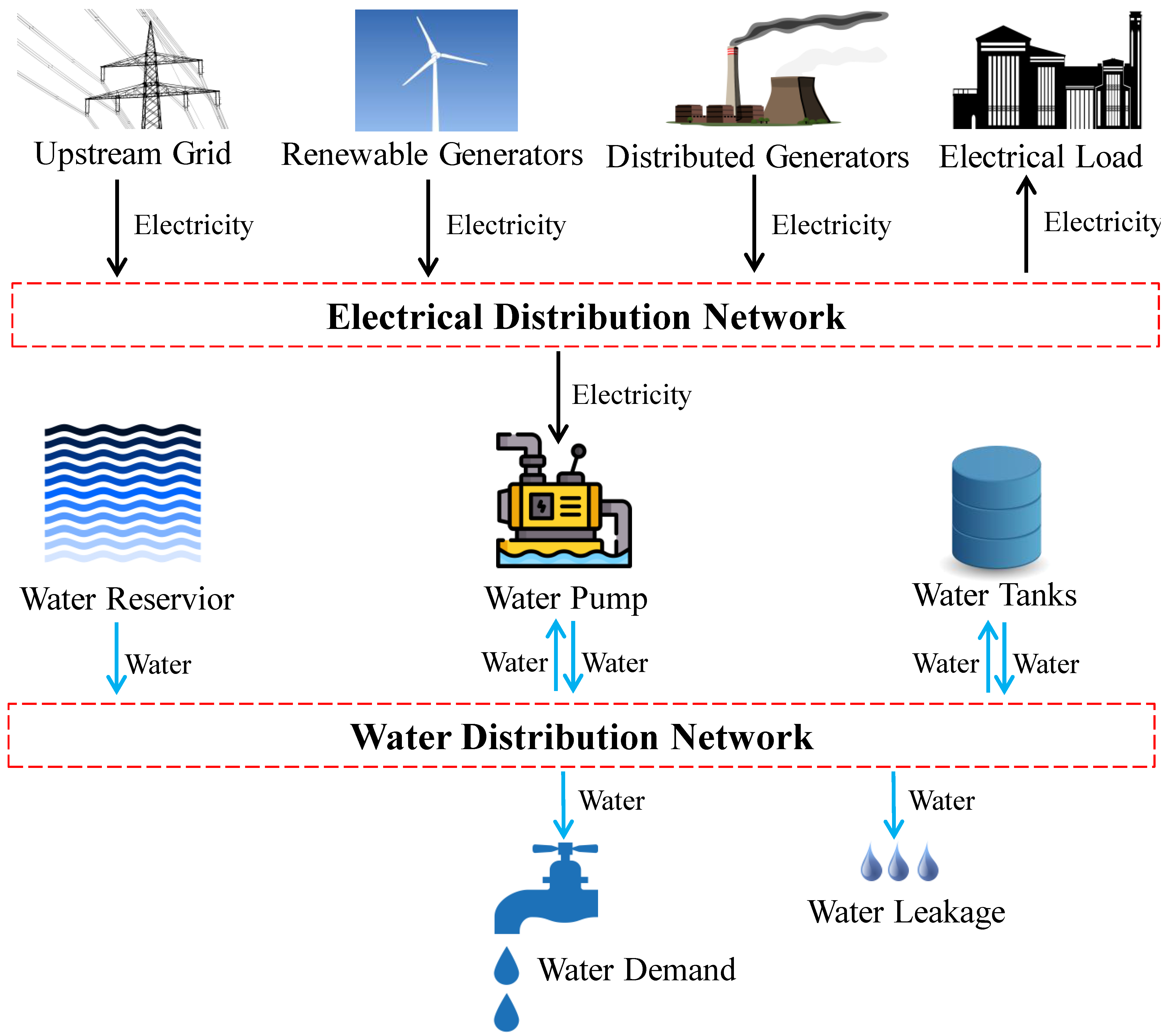
2. Cooperative Optimization Model of Water–Energy Nexus

In this section, the co-optimization model for the operation of the WEN is developed and presented in detail. The WEN in the proposed model includes the electrical distribution system and the water distribution system, as shown in Figure 1. The EDN delivers electricity from the upstream power grid, renewable generation (e.g., wind turbines), and conventional distributed generators (DGs) to supply the electrical loads including the pumps in the water distribution system. Meanwhile, the water demand is supplied by the water sources (e.g., water reservoir and tanks) through the WDN while the pumps are operated to maintain proper water head and flow in the pipes. Meanwhile, the water leakage in the WDN is considered in the proposed model.

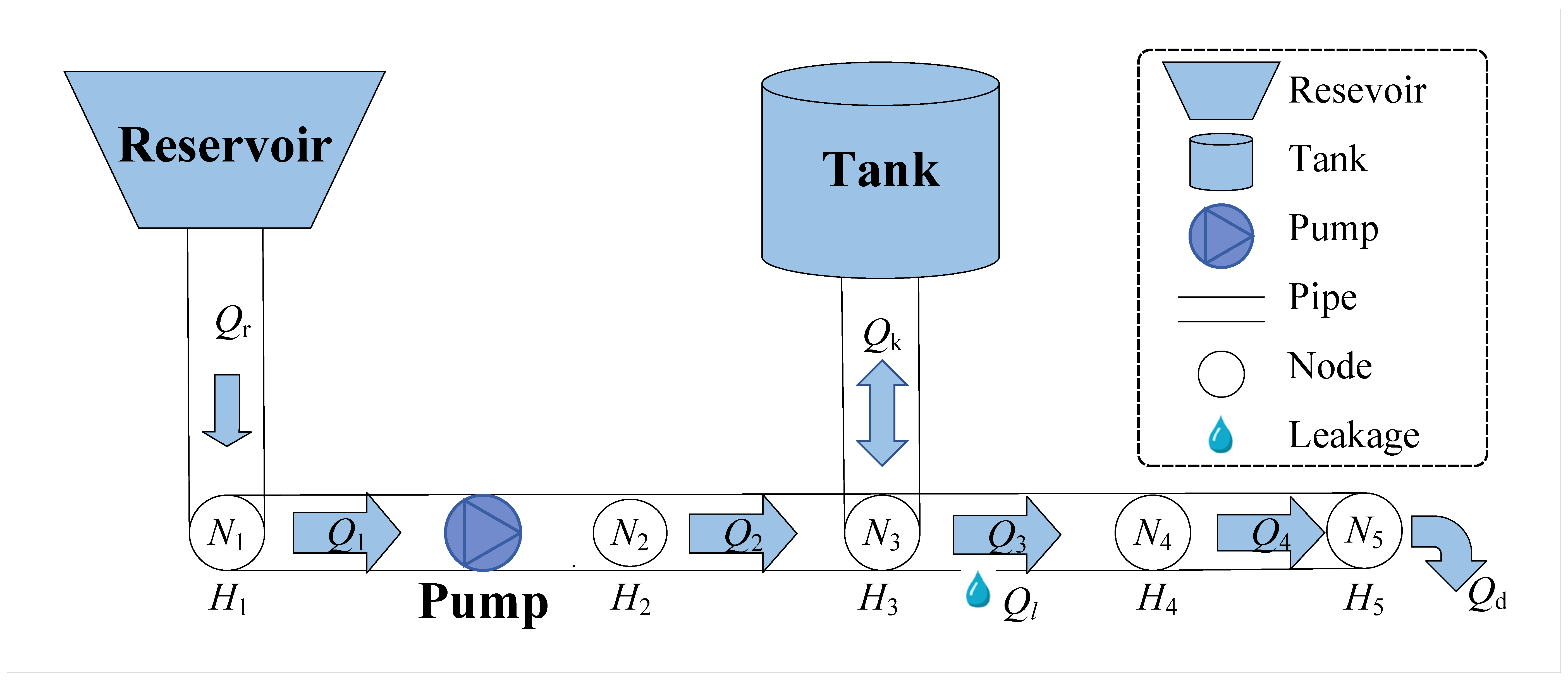
2.1. Configuration of Water Distribution System

The WDN can be represented by a directed graph G = ( N WDN , E WDN ) , as shown in Figure 2, which includes R reservoirs, P pipes, U pumps, K tanks, D water demand, and L leakage. N WDN = N J N RSV N TK is the set of N nodes including the set of reservoirs N RSV , tanks N TK , and connection nodes N J , while E WDN = E O E U is the set of E arcs (i.e., pipes) in the WDN that includes the sets of pipes without pumps E O and with pumps E U . In this paper, it is assumed that pumps are all installed in E U . Thus, E U can also represent the set of pumps in the WDN. T = 1 , , T is the set of scheduling time intervals in the proposed model.
In the WDN comprising interconnected pipes, pumps, and storage tanks, water is conveyed from the source to end-users, with potential losses occurring due to leakage along the pipeline infrastructure. At each node i N WDN in the WDN, the water head H i , t generally consists of two parts, including the pressure head due to the kinetic energy of the water, denoted by H i , t PRE , and the elevation head due to the gravitational potential energy, denoted by H i , t ELE . Thus, H i , t = H i , t PRE + H i , t ELE , i N WDN . Meanwhile, each arc j E WDN in the WDN has a certain water flow rate, denoted by Q j , t . The water flow rate in pipes is influenced simultaneously by the elevation difference between the nodes, the pressure head generated by the pumps, and the water head loss in pipes caused by friction.

2.1.1. Reservoir Constraints

H i , t = H i , t ELE i N RSV , t T
This equation defines the water head at reservoir nodes N R S V . Here, H i , t represents the hydraulic head at node i in time interval t, while H i , t E L E denotes the elevation head. This constraint is derived from the physical characteristic of reservoirs, which are typically modeled as infinite sources with fixed water levels. The assumption of constant head simplifies the hydraulic analysis and is widely adopted in WDN studies [26].

2.1.2. Water Tank Constraints

Q ¯ k Q k , t T K Q ¯ k k N T K , t T
Θ k , t = Θ k , t 1 + Q k , t T K t k N T K , t T
Θ ̲ k Θ k , t Θ ¯ k k N T K , t T
Equation (2a) restricts the flow rate Q k , t T K into/out of tank k to within the physical capacity limits ± Q ¯ k . This ensures that the tank’s inflow/outflow does not exceed the maximum rate allowed by connected pipes and pumps [27].
Equation (2b) represents the mass balance principle for tanks, where Θ k , t is the stored volume at time t, and t is the time step. This dynamic constraint captures the temporal dependency of tank levels.
Equation (2c) enforces the minimum and maximum storage limits Θ ̲ k and Θ ¯ k , preventing overflow or complete depletion. These constraints are fundamental for maintaining system reliability and are commonly used in WDN optimization.

2.1.3. Pumps Constraints

As the coupling component in the WEN, the water pumps consume electricity from the EDN and provide water head gain in the WDN.
H u , t P M = Ω u , t a u , 1 a u , 2 Q u , t Ω u , t a u , 3 u E U , t T
p u , t P M = Ω u , t 3 b u , 1 b u , 2 Q u , t Ω u , t u E U , t T
0 p u , t P M p ¯ u u E U , t T
0 Q u , t u E U , t T
Equation (3a) describes the pump head–flow relationship using an affinity law-based model, where H u , t P M is the head added by pump u at time t, and Ω u , t is the pump speed. Parameters a u , 1 , a u , 2 , and a u , 3 are pump-specific coefficients derived from manufacturer data [28]. Equation (3b) calculates the electrical power consumption p u , t P M as a cubic function of speed, reflecting the energy required to drive the pump. This model is widely used due to its accuracy in representing pump efficiency curves. Equations (3c) and (3d) ensure that pump operation stays within physical bounds: power consumption does not exceed the rated capacity p ¯ u , and flow rates are non-negative (preventing reverse flow). These constraints are critical for realistic pump modeling and energy optimization.

2.1.4. Node and Pipeline Constraints

In the WDN, the following equations govern the water head and flow-related constraints, each playing a crucial role based on the principles of water distribution system operation.
k : k i ε WDN Q k i , t + Q i , t RSV = j : i j ε WDN Q i j , t + Q i , t DM + Q i , t TK i N WDN , t T
Equation (4) represents the flow-balance constraint at nodes in the WDN. It enforces the principle of mass conservation, ensuring that k : k i ε WDN Q k i , t + Q i , t RSV , the total water inflow to node i at time t, is equal to j : i j ε WDN Q i j , t + Q i , t DM + Q i , t TK , the total outflow. This is fundamental for proper water distribution system operation.
H ̲ i H i , t H ¯ i i N WDN , t T
Equation (5) defines the bounds of the water head at each node i in the WDN at time t. The lower bound H ̲ i ensures sufficient pressure for water supply, while the upper bound H ¯ i safeguards the system against damage caused by excessive pressure.
Q ¯ i j Q i j , t Q ¯ i j i - j E WDN , t T
Equation (6) sets the flow-rate limits for pipes in the WDN. These limits, Q ¯ i j and Q ¯ i j , are determined by the physical capabilities of the pipes, ensuring that the flow rate Q i j , t remains within a safe and efficient range.
L i j , t = H i , t H j , t i - j E O , t T
For pipes without pumps ( i j E O ), Equation (7) calculates the head loss L i j , t based on the pressure drop due to friction between nodes i and j. It is a fundamental equation for analyzing energy loss in such pipes.
L i j , t = H i , t H j , t + H i j , t PM i - j E U , t T
In the case of pipes with pumps ( i j E U ), Equation (8) accounts for both the natural head loss H i , t H j , t and the pump-induced head gain H i j , t PM , providing a comprehensive model for head loss calculation.
L i j , t = F i j Q i j , t | Q i j , t | 1.852 i - j E WDN , t T
Equation (9) is the Hazen–Williams equation for head loss. It effectively estimates the head loss L i j , t in WDN pipes, especially for turbulent flow conditions. The resistance coefficient F i j , which is determined by the pipe’s material characteristics (as defined in Equation (10)), and the flow rate Q i j , t are used in this non-linear formula to calculate the head loss [29]. Q i j , t denotes the water flow of the pipe from node i to j at time t, Q i , t RSV is the water flow from the reservoir to node i at time t, Q i , t DM is the water demand at node i, Q i , t TK is the water flow to node i from the water tanks, L i j , t is the water head loss in pipe i j due to friction, H i , t is the water head at node i, H ̲ i and H ¯ i are the lower and upper bounds of the water head of node i, and F i j is the resistance coefficient of pipe i j , which is determined by the material characteristic of the pipe, as shown in Equation (10).
F i j = f i j l i j 2 d i j A i j 2 g i - j E WDN
Equation (10) calculates the resistance coefficient F i j of pipe i j . It is based on the pipe’s physical properties, including the friction coefficient f i j , length l i j , diameter d i j , cross-sectional area A i j , and the acceleration due to gravity g. This coefficient is essential for accurately determining the head loss in pipes as used in Equation (9). g is the acceleration due to gravity, f i j , l i j , d i j , and A i j are the friction coefficient, length, diameter, and area of pipe i j , respectively.

2.1.5. Water Leakage Constraints

Water leakage is a prevalent phenomenon in the management of WDN, causing considerable loss of water and energy from the moment that the leaks are formed. The relationship between the leakage rate and water head can be formulated by an exponential function as shown in Equation (11) below [30].
Q i j , t LK = λ LK H i j , t ϕ i j E WDN , t T
where Q i j , t LK is the leakage rate of pipe i j at time t, λ LK is the leakage coefficient, H i j , t is the average water head of pipe i j at time t, and ϕ is the leakage exponent.

2.2. Power Distribution Network Constraints

In this paper, a linearized DistFlow model is applied to formulate the power flow in the power distribution network of the WEN, which is widely used in the analysis of the energy management and optimal operation of electrical distribution systems and WEN [14].

2.2.1. Power Flow Constraints

In the EDN, the following equations describe the power flow and related constraints. Each equation has a distinct meaning and its selection is based on the fundamental principles of power system operation.
p t GD + d D i 0 p d , t DG + w W i 0 p w , t WT p i 0 , t EL u U i 0 p u , t PM = j : i 0 j E EDN p i 0 j , t t T
Equation (12) represents the active power balance constraint at the root bus i 0 . Ensuring the balance of active power at the root bus is crucial for maintaining the stability and proper operation of the entire distribution network. If the active power balance is not maintained, it can lead to power shortages, voltage instability, and inefficient operation of electrical equipment.
q t GD + d D i 0 q d , t DG q i 0 , t EL = j : i 0 j E EDN q i 0 j , t t T
Equation (13) is the reactive power balance constraint at the root bus i 0 . By maintaining the reactive power balance at the root bus, we can ensure that the voltage levels in the distribution network remain within an acceptable range, which is necessary for the proper operation of electrical devices.
d D i p d , t DG + w W i p w , t WT p i , t EL u U i p u , t PM = j : i j E EDN p i j , t i N EDN { i 0 } , t T
For buses other than the root bus ( i N EDN { i 0 } ), Equation (14) enforces the active power balance. Similar to the root bus active power balance equation, it sums up the active power sources (from distributed generators and renewable units) and subtracts the active power demands (loads and pumps) at a particular bus i.
d D i q d , t DG q i , t EL = j : i j E EDN q i j , t i N EDN { i 0 } , t T
Equation (15) is the reactive power balance constraint for buses other than the root bus. It ensures that the reactive power sources (from distributed generators) minus the reactive power demands (loads) at a bus i are equal to the reactive power flowing out of that bus.
V j , t = V i , t r i j p i j , t + x i j q i j , t V 0 i N EDN , i j E EDN , t T
Equation (16) describes the relationship between the voltages at two adjacent buses i and j in the distribution network. It shows how the voltage at bus j at time t, V j , t , is related to the voltage at bus i, V i , t , and the power flows (active p i j , t and reactive q i j , t ) between them. The terms r i j and x i j are the resistance and reactance of the line connecting the two buses, and V 0 is the rated voltage at the root bus.
p ¯ i j p i j , t p ¯ i j i j E EDN , t T
Equation (17) sets the limits for the active power flow p i j , t in the branches of the distribution network. The upper and lower limits p ¯ i j and p ¯ i j are determined by the physical capabilities of the transmission lines and associated equipment.
q ¯ i j q i j , t q ¯ i j i j E EDN , t T
Equation (18) sets the bounds for the reactive power flow q i j , t in the network branches. Similar to the active power flow limits, the upper and lower limits q ¯ i j and q ¯ i j are based on the equipment capabilities.
V ̲ V i , t V ¯ i N EDN , t T
Equation (19) defines the lower and upper limits for the voltage V i , t at each bus i in the distribution network. The lower limit V ̲ and the upper limit V ¯ are set based on the requirements of electrical equipment connected to the buses. p u , t PM denotes the active power demand of pump u at time t, and p i , t EL and q i , t EL are the active and reactive power of the electrical loads other than the pumps at bus i at time t, respectively; p i j , t and q i j , t are the active and reactive power flows from bus i to bus j, respectively; p ¯ i j and q ¯ i j are the upper limits of the active and reactive power flows of the branch from bus i to bus j, respectively; r i j and x i j are the resistance and reactance of the branch in the EDN from bus i to bus j, respectively; V i is the voltage at bus i, V 0 is the rated voltage at the root bus, and V ¯ and V ̲ are the upper and lower voltage limits, respectively.

2.2.2. Distributed Generator Constraints

The active and reactive power outputs of the DGs are constrained by their upper and bounds, respectively, as shown in Constraints (20) and (21).
0 p d , t DG p ¯ d DG d D , t T
q ̲ d DG q d , t DG q ¯ d DG d D , t T
where p ¯ d DG denotes the upper limit of the active power output of DG unit d, and q ¯ d DG and q ̲ d DG are the upper and lower limits of the reactive power output of DG unit d, respectively.

2.3. Optimal Operation Model of WEN

The optimal operation problem of the WEN can be formulated by an optimization model as follows.
min t T c t E p t GD + d D a d DG p d t DG + b d DG p d t DG + c d DG + c W Q t RSV
subjected to (1)–(21).
Equation (22) illustrates the objective function of the WEN to minimize the operational cost of the overall system, which consists of three parts: the first part is the cost for electricity procurement from the upstream power grid, where c t E denotes the electricity price from the upstream grid; the second part is the total operational cost of the distributed generators, where a d DG , b d DG , and c d DG are the coefficients of the generation cost of DG unit d; the last part represents the water procurement cost from the reservoir, where c W is the purchase price per cubic meter of water.

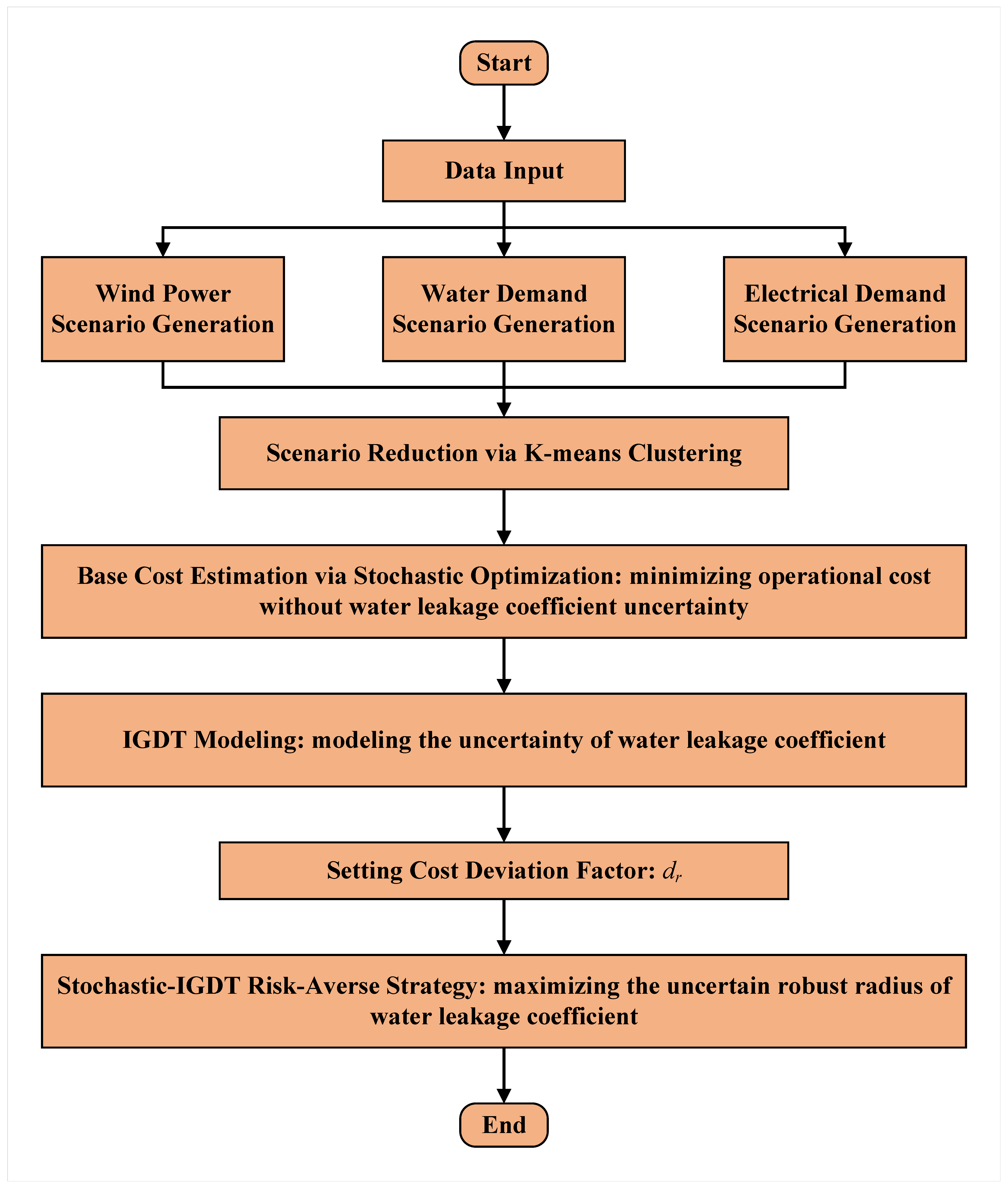
3. Hybrid Stochastic–IGDT Model of WEN Considering Leakage

The optimal operation of the WEN is challenging under the uncertainties associated with renewable generation, electrical loads, water demand, and potential water leakage in the WDN. Generally, there are rich analyses on the stochastic characteristics of renewable generation, electrical loads, and water demand. The probability distribution of these stochastic variables can be estimated and obtained from historical data. However, there is limited analysis on the stochastic characteristics of the leakage of the WDN for operation research [17]. Especially when the leakage is invisible, while it is possible to see potential leakage in one or a set of the pipes in the WDN, the detailed stochastic information of water leakage remains uncovered, which makes it difficult to use, and degrades the solution quality of using, optimization tools such as SO that depend on accurate stochastic information of the uncertain parameters [21,31]. To this end, a hybrid stochastic–IGDT model is proposed in this paper, in which an IGDT-based approach is developed to cope with the impacts of potential leakage in the WDN while the uncertainties from renewable generation, electrical loads, and water demand in the WEN are addressed using SO.

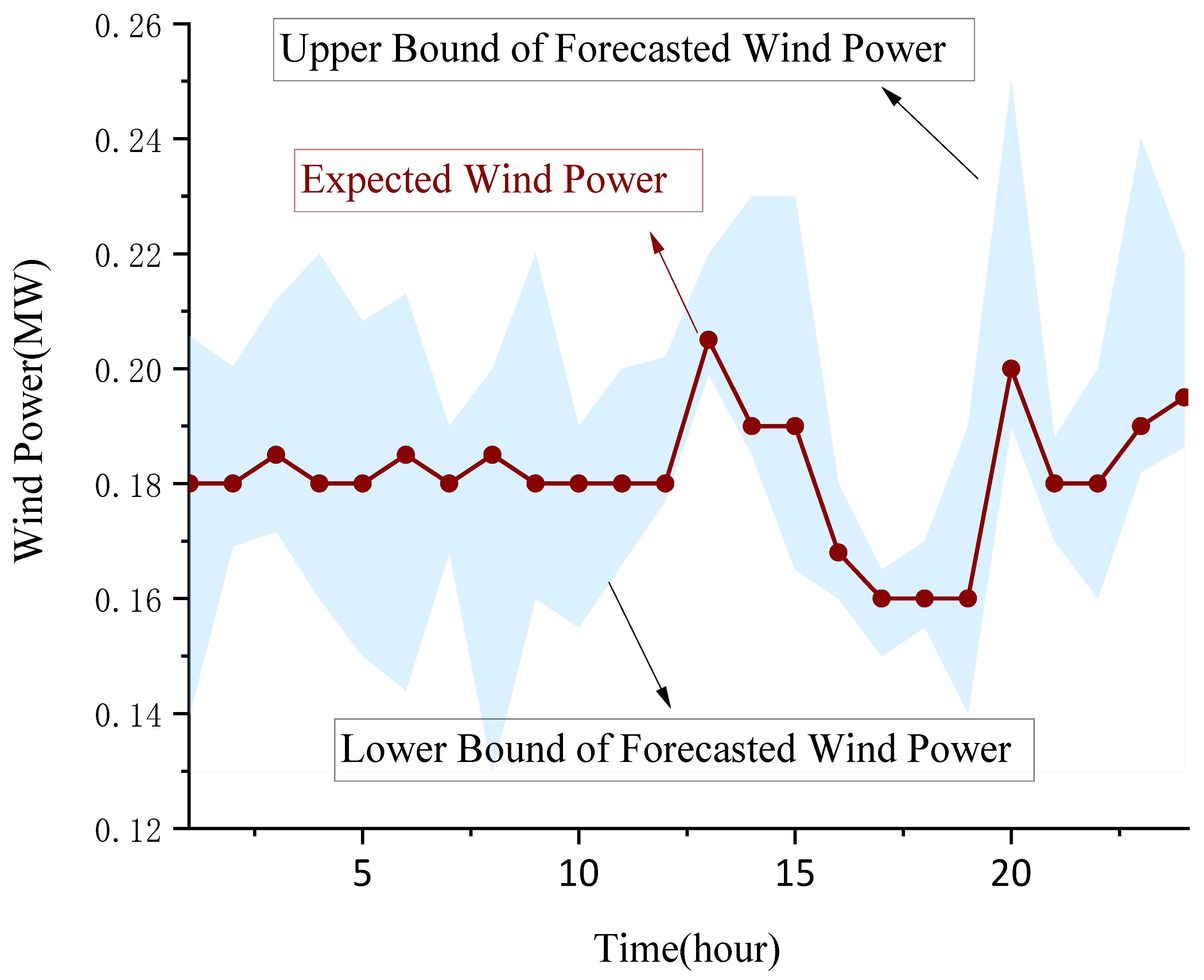
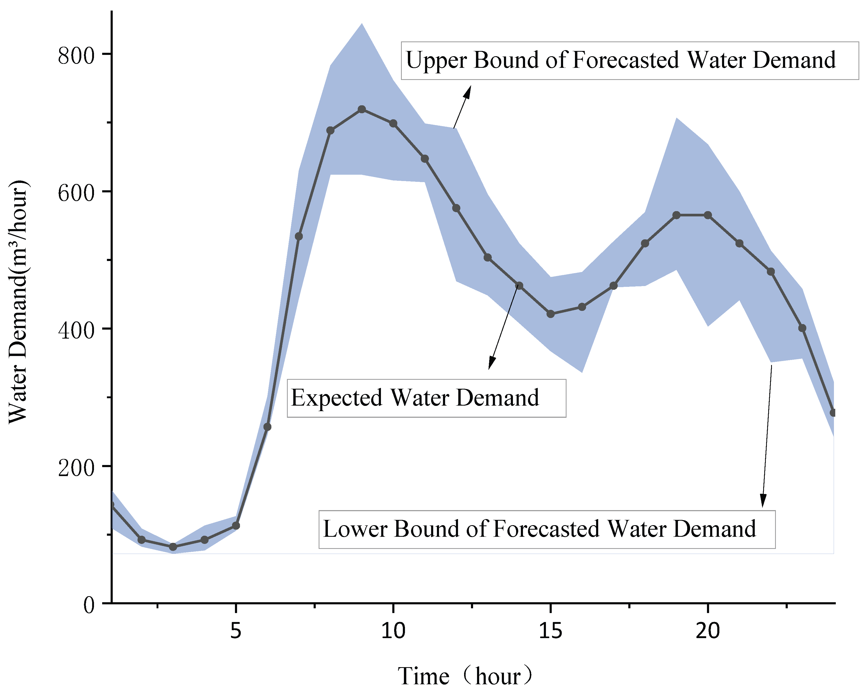
3.1. Probabilistic Uncertainty Modeling and Scenario Generation

The stochastic information concerning wind power, electrical demand, and water demand in the WEN is assumed to be available in this paper. The modeling of these stochastic variables can be presented as follows:
P w , t WT = P ^ w , t WT + P w , t Err , WT
P i , t EL = P ^ i , t EL + P i , t Err , EL
Q i , t DM = Q ^ i , t DM + Q i , t Err , DM
where P ^ w , t WT , P ^ i , t EL , and Q ^ i , t DM are the forecast or expected values of the output of wind turbine w, the electrical demand at node i in the EDN, and water demand at node i in the WDN, respectively; P w , t WT , P i , t EL , and Q i , t DM are the forecast errors of the wind generation, electrical demand, and water demand, respectively. Without loss of generality, P w , t WT , P i , t EL , and Q i , t DM are assumed to follow an independent normal distribution with a respective mean value and standard deviation [32]. For a scenario-based method, the set of uncertain scenarios can be generated through stochastic tools, e.g., Monte Carlo Simulation. In this paper, a set of uncertain scenarios is generated using Monte Carlo Simulation, and the K-mean clustering technique is applied to the scenario reduction process to obtain the typical uncertain scenario, limiting the number of scenarios for higher computational efficiency and performance while preserving the necessary elements of the original scenarios [33].

3.2. Stochastic Optimization Model

In the proposed hybrid stochastic–IGDT based model, a stochastic optimization problem of the WEN is first performed with a predicted leakage coefficient in the WDN to provide a baseline in the IGDT model.
The objective function of the stochastic optimization problem for the cooperative operation of the WEN can be obtained by reformulating model (22) as follows:
min Z cost SO = s S t T π s c t E p t GD + d D a d DG p d , t , s DG + b d DG p d , t , s DG + c d DG + c W Q t RSV
subject to (1)–(21) of all scenarios.
The SO model above minimizes the expected operational cost of the WEN to schedule the electricity procurement from the upstream grid and water procurement from the reservoir in the first stage and the output of the DGs in the second stage. By solving the SO problem above, the optimal solution for the operation of WEN considering the probabilistic uncertainties is obtained. Denote the optimal solution of the SO model by Z cost SO * = argmin Z cost SO . The obtained solution of the SO model will serve as a baseline to formulate the performance criterion in the IGDT model to cope with the potential leakage in the WDN.

3.3. Hybrid Stochastic–IGDT Optimization

Water leakage is a prevalent phenomenon in the water distribution system that can be hidden and difficult to allocate. Even though there are many water leakage detection techniques, it is still difficult to accurately describe leakage flow using explicit equations because water leakage has a complex relationship with the leakage location, the characteristics of the pipeline itself, and the water head at the leakage point [34]. Consequently, the leakage coefficient is often provided with an inaccurate value, making the scheduling decision of the SO mentioned above invalid. Thus, the fluctuation range of the leakage coefficient needs to be further considered. Without clear and accurate stochastic characteristics of the water leakage coefficient, SO and other optimization techniques that depend on the stochastic information of the uncertainties fall short in accurately formulating the impacts of potential leakage, while decisions derived from robust optimization tend to be overly conservative and misaligned with daily system operations [23]. To this end, this study employs the IGDT method to formulate the uncertainty of the leakage coefficient, aiming to identify an acceptable variation range given the operational cost limits, ensuring the operation decisions of the WEN remain valid and acceptable in performance under complex operational conditions. Furthermore, the IGDT-based method equips the WEN operator with the flexibility to adopt a risk-averse strategy when confronting uncertainties related to leakage [25,35].
The uncertainty set of the leakage coefficient λ LK can be formulated as follows:
Φ λ ˜ LK , α = λ LK : λ LK λ ˜ LK λ ˜ LK α , α 0
where α is the uncertainty horizon parameter and λ ˜ LK represents the estimated leakage coefficient. The constraint of the leakage coefficient with the uncertainty set as (27) can then be formulated as
( 1 α ) λ ˜ L λ L ( 1 + α ) λ ˜ L
The overall operational cost of the WEN can be determined as
Z cost = s S t T π s c t E p t GD + d D a d DG p d , t , s DG + b d DG p d , t , s DG + c d DG + c W Q t RSV
A risk-averse strategy is proposed in this study for the solution of the operation of the WEN. The risk-averse strategy desires to seek the largest uncertainty radius of the uncertainty quantity when the optimization aim falls into the permissible range, represented as follows:
max α
subject to (1)–(21) for all scenarios, (28), (29), and
Z cost ( 1 + d r ) Z cost SO *
where ( 1 + d r ) Z cost SO * represents the acceptable bound of the operational cost of the WEN in the risk-averse strategy, and d r is the robustness factor set by the WEN operator. The larger the value of the robustness factor, the less sensitive the scheme is to the fluctuation of the uncertainty quantity, the better the robustness of the model, and the stronger the risk avoidance ability of the WEN. Constraint (31) ensures that the operational cost of the WEN is bounded within the acceptable range while maximizing the tolerance of the strategy against potential water leakage conditions of the WDN. The overall procedure of the proposed hybrid stochastic–IGDT method for the risk-averse operation of WEN considering leakage is illustrated in Figure 3.

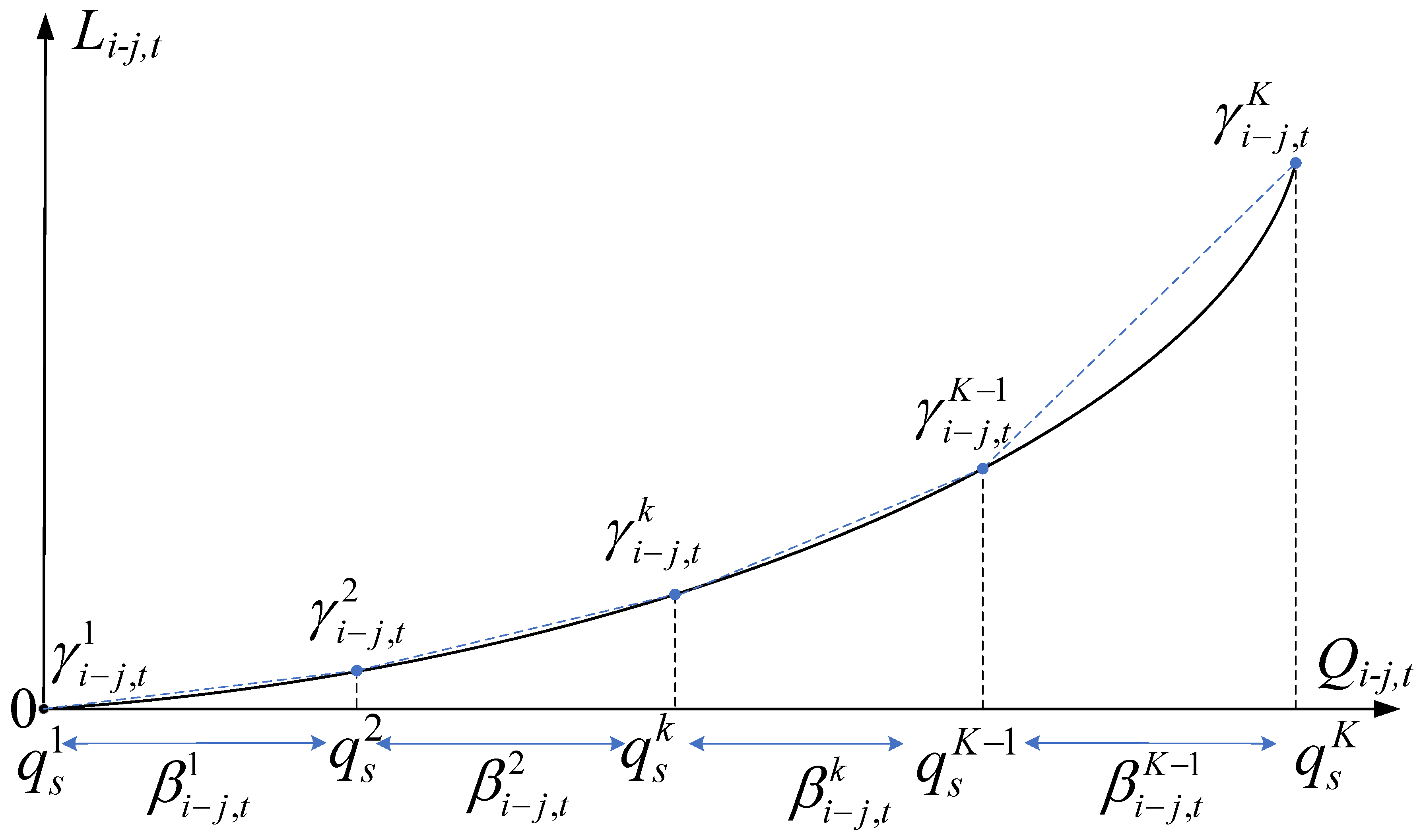
4. Linearization and Solution Method of Hybrid Stochastic–IGDT Model

The proposed hybrid stochastic–IGDT model of WEN presented in the previous sections is a nonlinear programming (NLP) problem due to the hydraulic constraints, which include the water head loss constraint (9), the water pumps’ operation constraints (3a)–(3b), and the leakage constraint (11). In order to support efficient solutions of the proposed model with off-the-shelf solves, a piece-wise linearization approach is applied to the nonlinear constraints in this study.
Constraint (9) illustrates the relationship between water head loss and the water flow. Figure 4 shows the hypothetical nonlinear water head loss function and the piece-wise linear approximation procedure [36]. Firstly, the Q i j axis is divided into K 1 segments evenly with K breakpoints. Each breakpoint k is associated with the sampling value of the water flow q i j 1 , q i j 2 , …, q i j K and a continuous variable γ i j , t k [ 0 , 1 ] . Each interval [ q i j k , q i j k + 1 ] is associated with a binary variable β i j , t k { 0 , 1 } .
Q i j , t = k = 1 K q i j k γ i j , t k
L ^ i j , t = k = 1 K L i j , t ( q i j k ) γ i j , t k
Every water flow segment q i j [ q i j k , q i j k + 1 ] can be represented by a linear combination of two consecutive breakpoints, q i j k and q i j k + 1 , weighted by the associated variable γ i j , t k , as shown by (32), and thus the water head loss L i j , t can be approximated by the linear function L ^ i j , t as a convex combination of the function values computed at the breakpoints q i j k and q i j k + 1 weighted by the same associated variables γ i j , t k , as shown by (33).
k = 1 K 1 β i j , t k = 1
k = 1 K γ i j , t k = 1
γ i j , t k β i j , t k 1 + β i j , t k k = 2 , , K 1
γ i j , t 1 β i j , t 1
γ i j , t K β i j , t K 1
0 γ i j , t k 1
Only a single line fragment is activated at the same time as a result of Constraint (34), which guarantees that merely a single binary variable β i j , t k may hold the value 1. Therefore, just a pair of consecutive positive continuous variables, γ i j , t k and γ i j , t k + 1 , are allowed to take non-zero values by constraints (35)–(39). As such, the water head loss constraint (9) is linearized. The leakage constraint (11) can be linearized similarly.
Constraints (3a) and (3b) show that the water head gain generated by pump u and the power consumed by pump u follow a nonlinear bivariate function associated with the speed of pump u and the water flow rate of pump u. As shown in Figure 5, the procedure of the linearization of Constraints (3a) and (3b) can therefore be performed using a convex combination triangulation method [36].
Firstly, the axis Q u , t is divided into N 1 segments evenly with N breakpoints, q u 1 , q u 2 , …, q u V , and the axis Ω u , t is divided into M 1 segments evenly with M breakpoints ω u 1 , ω u 2 , …, ω u M , where q u 1 and q u V as well as ω u 1 and ω u M coincide with the lower and upper bounds of the Q u , t and Ω u , t domains. Then, the functional domain of a bivariate function is partitioned into an array of rectangles. Consider the rectangle delineated by vertices ( q u v , ω u m ) , ( q u v + 1 , ω u m + 1 ) , ( q u v , ω u m + 1 ) , and ( q u v + 1 , ω u m + 1 ) , which is further segmented by diagonals into a pair of triangles defined by vertices ( q u v , ω u m ) , ( q u v , ω u m + 1 ) , and ( q u v , ω u m ) , ( q u v , ω u m + 1 ) . Each vertex ( v , m ) is associated with a continuous variable γ u , t ν , m within the [0, 1] interval, and binary variables, h ¯ u , t ν , m ( ν = 1 , , V 1 ; m = 2 , , M ) and h ̲ u , t ν , m ( ν = 2 , , V ; m = 1 , , M 1 ) , representing the apexes of the upper left and lower right triangles, respectively.
The locus of any pump’s operation point, constrained by q u ν Q u , t q u ν + 1 and ω u m Ω u , t ω u m + 1 , is uniquely defined by the linear amalgamations of the vertex coordinates, weighted by the pertinent variables γ u , t v , m , as dictated by Equations (40) and (41). The multivariate incremental functions h u , t ( Q u , t , Ω u , t ) and the power expressions P u , t W ( Q u , t , Ω u , t ) are thereafter linearly transfigured into h ^ u , t and P ^ u , t W as per Equations (42) and (43), which are in turn the convex combinations of the function values appraised at the triangle vertices encasing the operational point ( Q u , t , Ω u , t ) , with weighting by γ u , t v , m . Constraint (44) mandates that each resolution distinctly opts for a single triangle. Constraints (45) to (47) ensure that, in the majority of resolutions, no more than three of the continuous variables γ u , t v , m adopt non-zero magnitudes.
Q u , t = ν = 1 V m = 1 M q u ν γ u , t ν , m
Ω u , t = ν = 1 V m = 1 M ω u m γ u , t ν , m
h ^ u , t = ν = 1 V m = 1 M h u , t ( q u ν , ω u m ) γ u , t ν , m
P ^ u , t W = ν = 1 V m = 1 M P u , t W ( q u ν , ω u m ) γ u , t ν , m
ν = 1 V m = 1 M h ¯ u , t ν , m + h ̲ u , t ν , m = 1
ν = 1 V m = 1 M γ u , t ν , m = 1
γ u , t ν , m h ¯ u , t ν , m 1 + h ¯ u , t ν + 1 , m + h ¯ u , t ν , m + h ̲ u , t ν 1 , m + h ̲ u , t ν , m + 1 + h ̲ u , t ν , m ν , m
0 γ u , t ν , m 1 ν , m

5. Simulation and Discussions

In this section, case studies are used to demonstrate the effectiveness and applicability of the proposed co-optimization for the operation of the WEN considering leakage with the hybrid stochastic–IGDT approach.

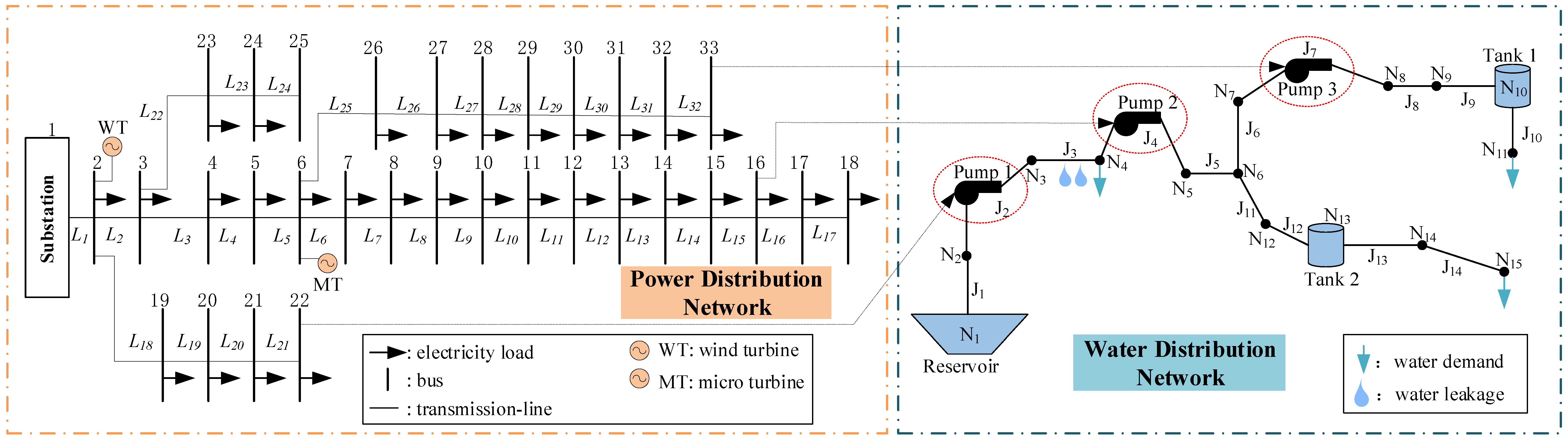
5.1. Key Parameters in Case Studies

The efficacy of the proposed robust operation model of WEN is evaluated on a test system with an EDN coupled with a WDN. The EDN in the test system is a modified IEEE 33-bus test system, which includes a micro-turbine connected to Bus 6 and a wind turbine connected to Bus 2. The WDN is a 15-node commercial-scale WDN that comprises 11 pipelines, two storage tanks, and three water demand nodes. Three pumps are installed in the WDN to provide necessary water head gain. They are connected to Buses 16, 22, and 33 of the EDN, respectively. The diagram of the test system of WEN in the case study is shown in Figure 6. The profile data for the EDN and WDN in the case study are provided in [37,38], respectively. Simulations in the case studies are performed using the Gurobi solver (version 10.0.3) on a desktop equipped with an Intel® Core™ i5-8500 CPU (Intel, Santa Clara, CA, USA), 8 GB of RAM, and a 64-bit operating system.
It is assumed in the case studies that the forecast errors in wind power, electrical demand, and water demand follow normal distributions: N ( 0 , ( 0.2 P WT ) 2 ) for wind power, N ( 0 , ( 0.1 P EL ) 2 ) for electrical loads, and N ( 0 , ( 0.1 Q DM ) 2 ) for water demand. A thousand original scenarios were generated using Monte Carlo Simulations and reduced to ten typical scenarios using the K-means clustering method to form the scenario set. The associated probabilities are listed in Table 2. The forecast wind power and water demand are shown in Figure 7 and Figure 8, respectively.
To better understand the scenarios in Table 2, let us take Scenario 5 and 9 as examples. Scenario 5, with a probability of 0.006, is the least likely. Its low probability implies a rare combination of wind power, electrical, and water demands. Here, variable values likely deviate greatly from expectations; for example, wind power could sharply differ from its mean, and electrical and water demands may fluctuate wildly. Such extreme combinations, though unlikely in practice, are accounted for due to the uncertainty modeled by Monte Carlo Simulation. Scenario 9, with a 0.260 probability, is the most likely. It represents the typical combination of these demands, serving as a benchmark for the system’s behavior under uncertainty. In this scenario, the values of wind power, electrical demand, and water demand deviate minimally and balancedly from their expected levels, reflecting common outcomes from the Monte Carlo Simulation.

5.2. Case Study Results

Four cases were simulated: Case I (independent WDN and EDN operation, no leakage), Case II (independent operation with leakage), Case III (WEN co-optimization, no leakage), and Case IV (WEN co-optimization with leakage in the fourth pipeline, leakage coefficient 3 × 10 5 ). Additionally, in order to examine the impacts of leakage positions on system operation, different leakage positions in the WDN with different various robustness coefficients were simulated. The results of the four respective cases are summarized in Table 3.
Table 2 shows that the comparison between Cases I and III demonstrates the effectiveness of the proposed WEN co-optimization model. It significantly reduces electrical energy consumption and cuts the operational cost by 23.01%. These results underscore the potential of integrated optimization strategies in improving system efficiency and reducing expenses. Comparisons between Cases I and II, as well as those between Cases III and IV, reveal that a leakage rate of 1–10% in individual water pipelines increases water procurement requirements by about 7% and 4%, respectively, leading to total operational cost increases of 4% and 3%. However, the comparison between Cases II and IV demonstrates that the joint optimization, which strategically coordinates the operation of pumps, water flow, and tanks, properly manages the hydraulic head in the WDN. Such adjustment minimizes the water loss due to the leakage, achieving a substantial reduction in total operational cost by CNY 28,201.29. These findings support coordinated optimization as a valuable approach for enhancing the efficiency and sustainability of the WEN.
To assess the impact of piece-wise linearization on optimization results and computational efficiency, we compared the outcomes of Case III using two methods: piece-wise linearization with five breakpoints and a non-linearized approach.
As shown in Table 4, the two methods have only a marginal difference in objective function values. Slight variations in power expense, purchased water volume, and total operational cost are within an acceptable range, indicating that the linearization error of piece-wise linearization has negligible impact on the final results. However, the computational performance differs significantly. Without linearization, the solving time increases from 120 s to 935 s, nearly tripling. This highlights the high computational burden of the non-linearized method, especially for more complex problems. In conclusion, piece-wise linearization balances computational efficiency and solution accuracy effectively. By sacrificing a small amount of precision, it greatly reduces the solving time.
Water leakage wastes resources and makes the traditional WEN co-optimization scheduling model infeasible. Figure 9 shows the difference between hourly water demand and supply when the fourth pipeline leaks (leakage coefficient 3 × 10 5 ), reflecting the impact of leakage on water supply. In the absence of leakage, the volume of water purchased from the reservoir should precisely match the total demand with the flow to/from the tanks. However, when leakage occurs in the pipeline without the operator’s awareness, as assumed in the traditional WEN model, approximately 10% of the water flow is lost (Case II), resulting in an insufficient supply.
As shown in Figure 6, the tested leaky pipe (Pipe 4) in the case studies is located downstream of the first pump, which raises the water head for the downstream network (Figure 10). Figure 11 shows that in the leakage scenario (Case IV), Pump 1 operates at a lower speed for the majority of the time, primarily to overcome friction between the water and the pipes, as well as head loss due to elevation. Such strategies are notably different with Case III, where Pump 1 occasionally operates at a much higher power consumption (approximately 195% more than in Case IV). As a result, the average head of the leaking pipe in Case IV is 52% lower than that in Case III, reducing the leakage rate and thus lowering the system’s operational costs. In contrast, since the leakage occurs upstream of Pumps 2 and 3, there is no need to strictly control the head at these nodes. Therefore, the power consumption of Pumps 2 and 3 in Case IV remains largely unchanged from that in Case III for most of the operational period, as shown in Figure 12.
In order to validate the resilience of the proposed hybrid stochastic–IGDT method, Case IV is solved using the hybrid stochastic–IGDT method and pure SO method under two conditions. Pipeline No.4 exhibits a nominal leakage coefficient of 3 × 10 5 (10% leakage rate) under normal conditions, but this coefficient may surge to 1.5 × 10 4 (47% leakage rate) due to unexpected corrosion or structural damage (Table 5). The SO method, which assumes a fixed leakage coefficient, fails to account for such fluctuations, leading to severe water shortages and an 18.1% cost increase from emergency responses. In contrast, the hybrid stochastic–IGDT method maintains 99% supply satisfaction with minimal deficits under extreme conditions and exhibits 0.01% cost resilience.
To investigate the impacts of the water leakage location and coefficient on water loss, scenarios with leakage in each pipe of the WDN were tested while the water leakage coefficients were set to 3 × 10 5 , 4 × 10 5 , and 5 × 10 5 in each scenario, respectively. The results are presented in Figure 13. It is indicated that the leakage amount is associated with the location of the leaking pipe. Generally, less water leakage occurs in the upstream (1st to 4th pipes), while relatively higher water leakage is observed in the middle and lower reaches (5–14th water pipes). Moreover, a larger leakage factor leads to a greater amount of water leakage.
The literature [31] indicates that while current technologies can accurately locate leaking pipes, precisely estimating the leakage rate remains challenging. In the model proposed in this paper, the pipeline leakage coefficient is set to 3 × 10 5 , corresponding to a leakage rate of approximately 1–10% of the original water flow rate. At this leakage rate, the minimum operational cost of the water–energy nexus system calculated via stochastic optimization serves as a baseline value. To assess the tolerance range of the uncertainty in the pipeline leakage coefficient within the hybrid stochastic-IGDT solution strategy, different system robustness coefficients ( d r = 0.01 , 0.02 , 0.03 , 0.04 ) were assigned to different water supply pipes, corresponding to acceptable operational cost increases of 1%, 2%, 3%, and 4%, respectively. The operation results of the proposed hybrid stochastic–IGDT framework in Case IV are presented in Figure 14, where the left-hand axis represents the maximum deviation rate of the leakage coefficient α , and the right-hand axis represents the normalized operational cost Z cost . These four figures, respectively, illustrate the impacts on the performance of the water–energy nexus system model when leakage occurs in (a) the first, (b) the fifth, (c) the ninth, and (d) the fourteenth water supply pipes. Overall, there is a positive correlation between the robustness factor d r and the deviation degree of the leakage coefficient, validating the core mechanism of the hybrid stochastic–IGDT framework to enhance system robustness by expanding the uncertainty tolerance range. Specifically, α for all water supply pipes increases significantly with the increase in d r . For example, α of the first water supply pipe increases from 6.1 × 10 5 to 14.1 × 10 5 , demonstrating an enhanced tolerance of the system to uncertainties.
The hydraulic characteristics of water supply pipes significantly influence the tolerance of pipeline leakage coefficient deviation. Upstream pipes, such as the first one, demonstrate the highest leakage tolerance ( α = 14.1 × 10 5 at d r = 0.04 ) due to their low-head conditions, which limit leakage volume and mitigate the impact on the water distribution network. In contrast, midstream pipes, like the fifth one, exhibit much lower α values ( 1.44 × 10 5 at d r = 0.04 ). High-head environments in these pipes lead to severe pressure drops upon leakage, triggering costly emergency measures, thus necessitating stricter α settings in the model. Downstream pipes, including the ninth and fourteenth ones, present moderate tolerance levels with α reaching 3.35 × 10 5 and 5.68 × 10 5 at d r = 0.04 . They can maintain acceptable cost increases by preferentially scheduling water tanks while expanding α . For example, the upstream pipe’s α can reach 14.1 × 10 5 with only a 4% cost increase at d r = 0.04 , exemplifying the trade-off between robustness and economy in different system regions. In summary, the proposed hybrid stochastic-IGDT approach ensures system effectiveness and feasibility even under wide-ranging leakage coefficient deviations. These findings underscore the need for customized risk management strategies in water distribution systems, tailored to the distinct characteristics and vulnerabilities of individual pipes. The method thus offers a robust framework for optimizing operational efficiency under multiple uncertainties.
The above findings highlight the significance of customized risk management strategies in water distribution systems, considering the unique characteristics and vulnerabilities of various pipeline segments. The hybrid stochastic-IGDT method emerges as an effective approach for enhancing system resilience against multiple uncertainties, offering a robust framework for optimizing operational efficiency amidst variable conditions.

6. Conclusions

This study presents a WEN cooperative operation model with a hybrid stochastic–IGDT method considering uncertainties and WDN leakage. Case studies show that integrating EDN and WDN optimization can improve system efficiency and reduce water waste and operational costs. It is also shown in the results that potential water leakage in the WDN can lead to sub-optimal or even infeasible solutions of the WEN operation model if it is not considered. The proposed hybrid stochastic–IGDT approach can effectively alleviate the impacts of probabilistic uncertainties from renewable generation, electrical loads, water demand, and the limited stochastic information of water leakage. The solution of the proposed method provides necessary robustness with a risk-averse strategy for the operation of the WEN. This cooperative optimization strategy of WEN not only bolsters the sustainability and reliability of the overall system but also offers valuable insights for the future design and operation of related integrated energy systems. The approach provides a framework for balancing the competing demands of water and energy resources, ensuring that both are managed in a way that minimizes environmental impacts, maximizes economic efficiency, and handles complex operational conditions.
Future research may expand the WEN model to include other energy systems from an IES perspective, which could provide more operational flexibility and significantly influence the operational decisions. Additionally, incorporating advanced detection and localization techniques for pipe leakages will be considered to further improve the model’s ability to respond to real-time operational conditions and reduce water and energy waste. Furthermore, additional studies will be performed focusing on the operational stability and reliability of interconnected WENs, particularly in the context of increasing climate variability and the growing demand for both water and energy resources.

Author Contributions

Conceptualization, J.Z., Z.L. and Q.-H.W.; methodology, J.Z. and Z.L.; software, J.Z.; validation, J.Z. and Z.L.; formal analysis, J.Z. and Z.L.; investigation, J.Z.; resources, Z.L. and Q.-H.W.; data curation, J.Z. and Z.L.; writing—original draft preparation, J.Z.; writing—review and editing, J.Z. and Z.L.; visualization, J.Z. and Z.L.; supervision, Z.L. and Q.-H.W.; project administration, Z.L.; funding acquisition, Z.L. All authors have read and agreed to the published version of the manuscript.

Funding

This research is supported by the Guangdong Basic and Applied Basic Research Foundation (Program No. 2023A1515011171).

Institutional Review Board Statement

Not applicable.

Informed Consent Statement

Not applicable.

Data Availability Statement

The data can be found in References [37,38].

Conflicts of Interest

The authors declare no conflicts of interest.

Nomenclature

T Set of scheduling time intervals
N WDN Set of nodes in the water distribution network
N RSV Set of reservoir nodes in the water distribution network
N TK Set of water tank nodes in the water distribution network
E WDN Set of pipes in the water distribution network
E O Set of pipes without pumps in the water distribution network
E U Set of pipes with pumps in the water distribution network (equivalent to the set of pumps)
N EDN Set of nodes in the electrical distribution network
E EDN Set of branches in the electrical distribution network
D Set of distributed generators
D i Set of distributed generators connected to node i in the electrical distribution network
W Set of renewable generation units (e.g., wind turbines)
W i Set of renewable generation units installed at node i in the electrical distribution network
U Set of pumps
U i Set of pumps connected to node i in the electrical distribution network
H i , t Water head at node i in the water distribution network at time t
H i , t E L E Elevation head at node i in the water distribution network at time t
H ̲ i Lower bound of water head at node i in the water distribution network
H ¯ i Upper bound of water head at node i in the water distribution network
Q k i , t Water flow from node k to node i at time t
Q i , t RSV Water flow from the reservoir to node i at time t
Q i , t DM Water demand at node i in the water distribution network at time t
Q i , t TK Water flow between the water tank and node i (inflow or outflow) at time t
Q k , t TK Flow rate of water tank k at time t
Q ¯ k Maximum flow rate of water tank k
Θ k , t Stored water volume in water tank k at time t
Θ ̲ k Lower bound of stored water volume in water tank k
Θ ¯ k Upper bound of stored water volume in water tank k
t Duration of each time interval
H u , t PM Head added by pump u at time t
Ω u , t Speed of pump u at time t
a u , 1 , a u , 2 , a u , 3 Pump - specific parameters of pump u (used in the head - flow model)
b u , 1 , b u , 2 Pump-specific parameters of pump u (used in the power-flow model)
p u , t PM Electrical power consumption of pump u at time t
p d , t DG Active power output of distributed generator d at time t
q d , t DG Reactive power output of distributed generator d at time t
p w , t WT Active power output of wind turbine w at time t
p i , t EL Active power demand of electrical loads (excluding pumps) at node i in the electrical distribution network at time t
q i , t EL Reactive power demand of electrical loads (excluding pumps) at node i in the electrical distribution network at time t
p i j , t Active power flow from node i to node j in the electrical distribution network at time t
q i j , t Reactive power flow from node i to node j in the electrical distribution network at time t
p ¯ i j Upper limit of active power flow in branch i j of the electrical distribution network
q ¯ i j Upper limit of reactive power flow in branch i j of the electrical distribution network
r i j Resistance of branch i j in the electrical distribution network
x i j Reactance of branch i j in the electrical distribution network
V i , t Voltage at node i in the electrical distribution network at time t
V 0 Rated voltage at the root bus of the electrical distribution network
V ̲ Lower limit of voltage in the electrical distribution network
V ¯ Upper limit of voltage in the electrical distribution network
c t E Price of electricity procurement from the upstream grid at time t
a d D G , b d D G , c d D G Generation cost coefficients of distributed generator d
c W Purchase price per cubic meter of water from the reservoir
P w , t W T Actual output power of wind turbine w at time t
P ^ w , t W T Predicted or expected output power of wind turbine w at time t
P w , t E r r , W T Forecast error of wind generation of wind turbine w at time t
P i , t E L Actual electrical load power at node i in the electrical distribution network at time t
P ^ i , t E L Predicted or expected electrical load power at node i in the electrical distribution network at time t
P i , t E r r , E L Forecast error of electrical load power at node i in the electrical distribution network at time t
Q i , t D M Actual water demand at node i in the water distribution network at time t
Q ^ i , t D M Predicted or expected water demand at node i in the water distribution network at time t
Q i , t E r r , D M Forecast error of water demand at node i in the water distribution network at time t
λ L K Leakage coefficient of pipes in the water distribution network
Φ λ ˜ L K , α Uncertainty set of the leakage coefficient λ L K
λ ˜ L K Estimated leakage coefficient
α Uncertainty horizon parameter (uncertainty radius in IGDT)
d r Robustness factor set by the WEN operator
Z c o s t S O Expected operational cost of the WEN in the stochastic optimization model
Z c o s t S O * Optimal solution of the stochastic optimization model (when minimizing the expected operational cost)
Z c o s t Actual operational cost of the WEN considering leakage uncertainty
π s Probability of scenario s
L i j , t Water head loss in pipe i j in the water distribution network at time t
F i j Resistance coefficient of pipe i j in the water distribution network
f i j Friction coefficient of pipe i j in the water distribution network
l i j Length of pipe i j in the water distribution network
d i j Diameter of pipe i j in the water distribution network
A i j Cross - sectional area of pipe i j in the water distribution network
gAcceleration due to gravity
Q i j , t L K Leakage rate of pipe i j in the water distribution network at time t
ϕ Leakage exponent (exponent used to describe the relationship between leakage rate and water head)
p t G D Active power exchange between the upstream grid and the electrical distribution network at time t
q t G D Reactive power exchange between the upstream grid and the electrical distribution network at time t
p ¯ d D G Upper limit of active power output of distributed generator d
q ¯ d D G Upper limit of reactive power output of distributed generator d
q ̲ d D G Lower limit of reactive power output of distributed generator d
β i j , t k Binary variable used for the linearization of the water head loss constraint in the water distribution network (related to pipe i j , time t, and segment k)
γ i j , t k Continuous variable used for the linearization of the water head loss constraint in the water distribution network (related to pipe i j , time t, and segment k)
q i j k Sampling value of water flow for the linearization of the water head loss function of pipe i j in the water distribution network
L ^ i j , t Linear approximation of water head loss in pipe i j at time t in the water distribution network
γ u , t v , m 
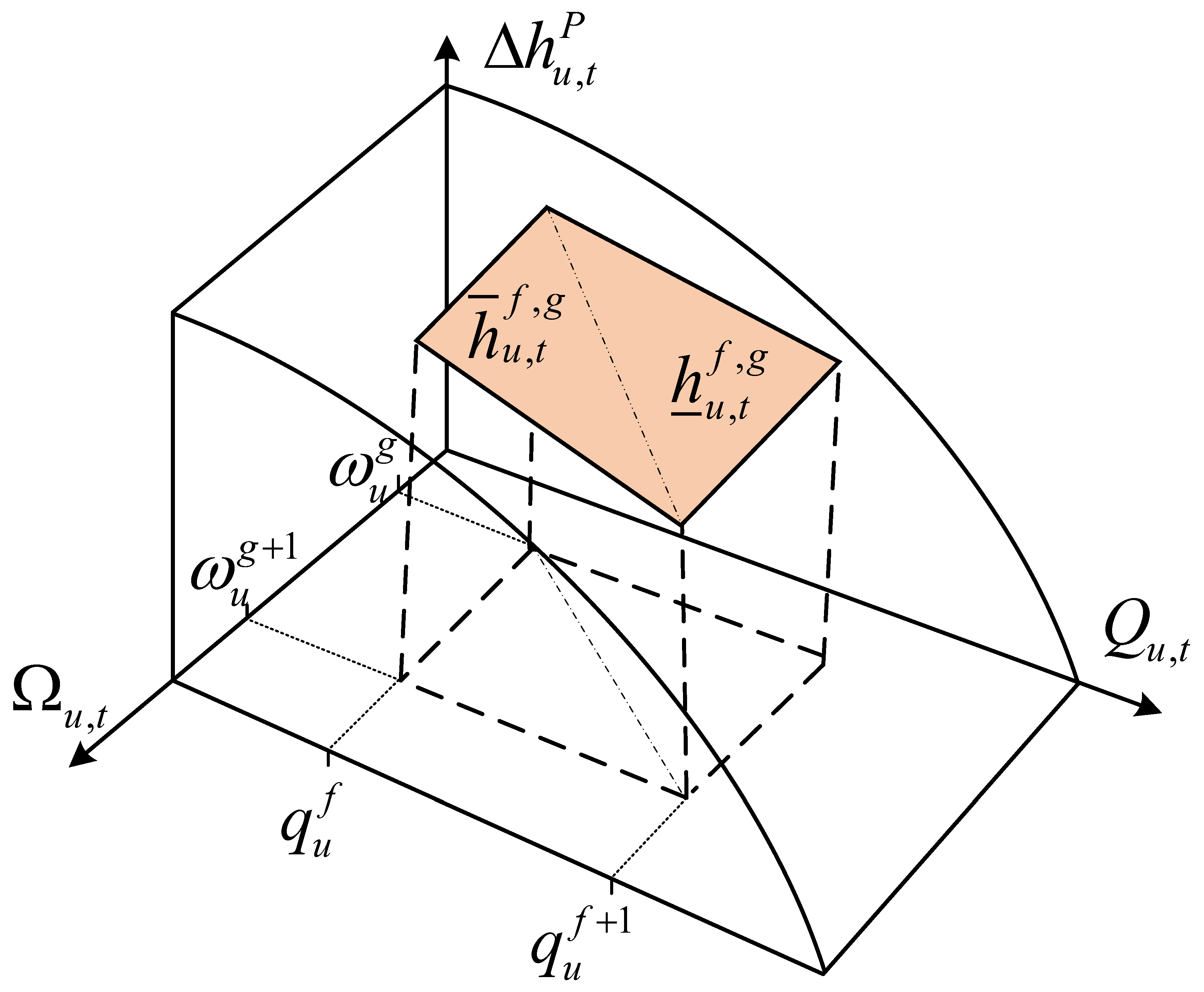
Continuous variable related to pump u, time t, and coordinates ( v , m ) for the linearization of pump-related constraints
h ¯ u , t v , m Binary variable related to pump u, time t, and coordinates ( v , m ) for the linearization of pump-related constraints (representing the upper-left triangle vertex)
h ̲ u , t v , m Binary variable related to pump u, time t, and coordinates ( v , m ) for the linearization of pump-related constraints (representing the lower - right triangle vertex)
q u v Sampling value of pump u’s water flow for the linearization of pump - related constraints
ω u m Sampling value of pump u’s speed for the linearization of pump - related constraints
h ^ u , t Linear approximation of the head gain of pump u at time t
P ^ u , t W Linear approximation of the power consumption of pump u at time t
CVaRConditional Value-at-Risk
DGDistributed generator
DRODistributionally robust optimization
EDNElectrical distribution network
IGDTInformation gap decision theory
IESIntegrated energy system
LPLinear programming
MINLPMixed - integer nonlinear programming
NLPNonlinear programming
RORobust optimization
SOStochastic optimization
WDNWater distribution network
WENWater - Energy Nexus

References

  1. Birol, F. World Energy Outlook 2016; IEA: Paris, France, 2016. [Google Scholar]
  2. Denig-Chakroff, D. Reducing Electricity Used for Water Production: Questions State Commissions Should Ask Regulated Utilities; National Regulatory Research Institute: Columbus, OH, USA, 2008. [Google Scholar]
  3. Tan, X.; Abedi, M.; Klausner, J.F.; Bénard, A. Modeling and experimental validation of light-splitting semi-transparent solar water heater using NIR cut-off film as the rooftop of a greenhouse for arid regions. Appl. Energy 2024, 368, 123489. [Google Scholar] [CrossRef]
  4. Busby, J.W.; Baker, K.; Bazilian, M.D.; Gilbert, A.Q.; Grubert, E.; Rai, V.; Rhodes, J.D.; Shidore, S.; Smith, C.A.; Webber, M.E. Cascading risks: Understanding the 2021 winter blackout in Texas. Energy Res. Soc. Sci. 2021, 77, 102106. [Google Scholar] [CrossRef]
  5. Gao, L.; Han, X.; Chen, X.; Liu, B.; Li, Y. The Spring Drought in Yunnan Province of China: Variation Characteristics, Leading Impact Factors, and Physical Mechanisms. Atmosphere 2023, 14, 294. [Google Scholar] [CrossRef]
  6. Oikonomou, K.; Parvania, M. Optimal coordinated operation of interdependent power and water distribution systems. IEEE Trans. Smart Grid 2020, 11, 4784–4794. [Google Scholar] [CrossRef]
  7. Zamzam, A.S.; Dall’Anese, E.; Zhao, C.; Taylor, J.A.; Sidiropoulos, N.D. Optimal Water–Power Flow-Problem: Formulation and Distributed Optimal Solution. IEEE Trans. Control Netw. Syst. 2019, 6, 37–47. [Google Scholar] [CrossRef]
  8. Kernan, R.; Liu, X.; McLoone, S.; Fox, B. Demand side management of an urban water supply using wholesale electricity price. Appl. Energy 2017, 189, 395–402. [Google Scholar] [CrossRef]
  9. Alnahhal, Z.; Shaaban, M.F.; Hamouda, M.A.; Majozi, T.; Bardan, M.A. A Water-Energy Nexus Approach for the Co-Optimization of Electric and Water Systems. IEEE Access 2023, 11, 28762–28770. [Google Scholar] [CrossRef]
  10. Li, Q.; Yu, S.; Al-Sumaiti, A.; Turitsyn, K. Micro Water-Energy Nexus: Optimal Demand-Side Management and Quasi-Convex Hull Relaxation. IEEE Trans. Control Netw. Syst. 2019, 6, 1313–1322. [Google Scholar] [CrossRef]
  11. Li, Q.; Yu, S.; Al-Sumaiti, A.; Turitsyn, K. Modeling and Co-Optimization of a Micro Water-Energy Nexus for Smart Communities. In Proceedings of the 2018 IEEE PES Innovative Smart Grid Technologies Conference Europe (ISGT-Europe), Sarajevo, Bosnia and Herzegovina, 21–25 October 2018; pp. 1–5. [Google Scholar]
  12. Fang, S.; Wang, C.; Lin, Y.; Zhao, C. Optimal Energy Scheduling and Sensitivity Analysis for Integrated Power–Water–Heat Systems. IEEE Syst. J. 2021, 16, 5176–5187. [Google Scholar] [CrossRef]
  13. Yu, D.; Li, Z.; Fan, S.; Sun, T. Optimal management of an energy-water-carbon nexus employing carbon capturing and storing technology via downside risk constraint approach. J. Clean. Prod. 2023, 418, 138168. [Google Scholar] [CrossRef]
  14. Zhao, P.; Gu, C.; Cao, Z.; Ai, Q.; Xiang, Y.; Ding, T.; Lu, X.; Chen, X.; Li, S. Water-energy nexus management for power systems. IEEE Trans. Power Syst. 2020, 36, 2542–2554. [Google Scholar] [CrossRef]
  15. Zhao, P.; Li, S.; Hu, P.J.H.; Gu, C.; Lu, S.; Ding, S.; Cao, Z.; Xie, D.; Xiang, Y. Blockchain-Based Water-Energy Transactive Management With Spatial-Temporal Uncertainties. IEEE Trans. Smart Grid 2023, 14, 2903–2920. [Google Scholar] [CrossRef]
  16. Wang, C.; Gao, N.; Wang, J.; Jia, N.; Bi, T.; Martin, K. Robust Operation of a Water-Energy Nexus: A Multi-Energy Perspective. IEEE Trans. Sustain. Energy 2020, 11, 2698–2712. [Google Scholar] [CrossRef]
  17. Audits, E.W. Water Loss Control for Public Water Systems; US EPA: Washington, DC, USA, 2013. [Google Scholar]
  18. Rogers, D. Leaking water networks: An economic and environmental disaster. Procedia Eng. 2014, 70, 1421–1429. [Google Scholar] [CrossRef]
  19. Valek, A.M.; Sušnik, J.; Grafakos, S. Quantification of the urban water-energy nexus in México City, México, with an assessment of water-system related carbon emissions. Sci. Total Environ. 2017, 590, 258–268. [Google Scholar] [CrossRef]
  20. Liemberger, R.; Wyatt, A. Quantifying the global non-revenue water problem. Water Supply 2019, 19, 831–837. [Google Scholar] [CrossRef]
  21. Zeng, J.; Liu, Z. Co-Optimization of Water-Energy Nexus Systems and Challenges. Eng. Proc. 2024, 69, 54. [Google Scholar]
  22. Powell, W.B. A unified framework for stochastic optimization. Eur. J. Oper. Res. 2019, 275, 795–821. [Google Scholar] [CrossRef]
  23. Ben-Tal, A.; El Ghaoui, L.; Nemirovski, A. Robust Optimization; Princeton University Press: Princeton, NJ, USA, 2009; Volume 283. [Google Scholar]
  24. Chow, Y.; Tamar, A.; Mannor, S.; Pavone, M. Risk-sensitive and robust decision-making: A cvar optimization approach. Adv. Neural Inf. Process. Syst. 2015, 28. [Google Scholar]
  25. Jordehi, A.R.; Javadi, M.S.; Shafie-khah, M.; Catalão, J.P. Information gap decision theory (IGDT)-based robust scheduling of combined cooling, heat and power energy hubs. Energy 2021, 231, 120918. [Google Scholar] [CrossRef]
  26. Guo, Y.; Wang, S.; Taha, A.F.; Summers, T.H. Optimal pump control for water distribution networks via data-based distributional robustness. IEEE Trans. Control Syst. Technol. 2022, 31, 114–129. [Google Scholar] [CrossRef]
  27. Alhazmi, M.; Dehghanian, P.; Nazemi, M.; Oikonomou, K. Uncertainty-informed operation coordination in a water-energy nexus. IEEE Trans. Ind. Inform. 2022, 19, 6439–6449. [Google Scholar] [CrossRef]
  28. Rodriguez-Garcia, L.; Hosseini, M.M.; Mosier, T.M.; Parvania, M. Resilience Analytics for Interdependent Power and Water Distribution Systems. IEEE Trans. Power Syst. 2022, 37, 4244–4257. [Google Scholar] [CrossRef]
  29. Liou, C.P. Limitations and proper use of the Hazen-Williams equation. J. Hydraul. Eng. 1998, 124, 951–954. [Google Scholar] [CrossRef]
  30. Schwaller, J.; van Zyl, J.V. Modeling the pressure-leakage response of water distribution systems based on individual leak behavior. J. Hydraul. Eng. 2015, 141, 04014089. [Google Scholar] [CrossRef]
  31. Sousa, J.; Martinho, N.; Muranho, J.; Marques, A.S. Leakage Calibration in Water Distribution Networks with Pressure-Driven Analysis: A Real Case Study. Environ. Sci. Proc. 2020, 2, 59. [Google Scholar]
  32. McQueen, D.H.; Hyland, P.R.; Watson, S.J. Monte Carlo simulation of residential electricity demand for forecasting maximum demand on distribution networks. IEEE Trans. Power Syst. 2004, 19, 1685–1689. [Google Scholar] [CrossRef]
  33. Sannigrahi, S.; Ghatak, S.R.; Acharjee, P. Multi-Scenario Based Bi-Level Coordinated Planning of Active Distribution System Under Uncertain Environment. IEEE Trans. Ind. Appl. 2020, 56, 850–863. [Google Scholar] [CrossRef]
  34. Ekmekcioğlu, Ö.; Başakın, E.E.; Özger, M. Discharge coefficient equation to calculate the leakage from pipe networks. J. Inst. Sci. Technol. 2020, 10, 1737–1746. [Google Scholar] [CrossRef]
  35. Mohammadi-Ivatloo, B.; Zareipour, H.; Amjady, N.; Ehsan, M. Application of information-gap decision theory to risk-constrained self-scheduling of GenCos. IEEE Trans. Power Syst. 2013, 28, 1093–1102. [Google Scholar] [CrossRef]
  36. Lin, M.H.; Carlsson, J.G.; Ge, D.; Shi, J.; Tsai, J.F. A review of piecewise linearization methods. Math. Probl. Eng. 2013, 2013, 101376. [Google Scholar] [CrossRef]
  37. Baran, M.E.; Wu, F.F. Network reconfiguration in distribution systems for loss reduction and load balancing. IEEE Trans. Power Deliv. 1989, 4, 1401–1407. [Google Scholar] [CrossRef]
  38. Oikonomou, K.; Parvania, M. Optimal Coordination of Water Distribution Energy Flexibility with Power Systems Operation. IEEE Trans. Smart Grid 2019, 10, 1101–1110. [Google Scholar] [CrossRef]
Figure 1. Schematic diagram of typical WEN.
Electronics 14 02644 g001
Figure 2. Schematic diagram of water distribution network.
Electronics 14 02644 g002
Figure 3. Schematic of the proposed hybrid stochastic–IGDT method.
Electronics 14 02644 g003
Figure 4. Piecewise linear approximation of pressure head loss function.
Electronics 14 02644 g004
Figure 5. Geometric representation of convex combination triangulation method applied to pump water head gain constraints.
Electronics 14 02644 g005
Figure 6. WEN model: modified IEEE 33-bus system with a 15-node commercial WDN.
Electronics 14 02644 g006
Figure 7. Forecast wind power scenarios.
Electronics 14 02644 g007
Figure 8. Forecast water demand scenarios.
Electronics 14 02644 g008
Figure 9. Hourly water demand in all cases and water supply of node 4 in Case IV.
Electronics 14 02644 g009
Figure 10. Daily average water head of each pipe in Case III.
Electronics 14 02644 g010
Figure 11. Comparison of average water head of pipe 4 and power consumed by pump 1 in Case III and Case IV.
Electronics 14 02644 g011
Figure 12. Comparison of power consumed by pump 2 and pump 3 in Case III and Case IV.
Electronics 14 02644 g012
Figure 13. Comparison of water loss caused by different leakage locations and leakage coefficients in 24 h.
Electronics 14 02644 g013
Figure 14. Robustness function of α vs. cost deviation factor ( d r ) in Case IV.
Electronics 14 02644 g014
Table 1. Comparison of uncertainty optimization methods.
MethodProbability DependencyKey AdvantagesMain Limiltation
SOStrong (requires
distribution)
Statistically
modeled uncertainty
Sensitive to distribution
errors and high computational cost
RONone (bounds only)Worst-case feasibilityOverly conservative solutions
CVaRStrong (requires
distribution)
Tail risk controlDistribution sensitivity
IGDTNone (bounds only)Handle distribution-free
uncertainties
Parameter sensitivity and
cannot utilize the probability
Hybrid
Stochastic
-IGDT
PartialHandles mixed
uncertainties
Complex model structure
Table 2. Probabilities of scenarios with uncertainty of wind power, electrical load, and water demand.
Scenario No.
Probability
1
0.200
2
0.073
3
0.034
4
0.027
5
0.006
Scenario No.
Probability
6
0.066
7
0.100
8
0.134
9
0.260
10
0.100
Table 3. Summary of optimization results in different cases.
CaseCo-OptimizedLeakage ConsideredPower Expense (CNY)Purchased Water (m3)Total Operational Cost (CNY)
Case I××70,861.4530,795.54117,054.76
Case II×73,348.2232,274.93121,760.62
Case III×43,842.3130,795.5490,035.62
Case IV45,288.5932,180.4993,559.33
Table 4. Comparison of optimization performance under different solution methods for Case III.
ApproachPower Expense (CNY)Purchased Water (m3)Total Cost (CNY)Solving Time (s)
Piecewise Linearization43,842.3130,795.5490,035.62120.52
Non-Linearized43,839.7830,802.3290,042.37935.43
Table 5. Comparison of performance between SO and hybrid stochastic–IGDT methods under leakage uncertainty.
Comparison IndicatorSOHybrid Stochastic–IGDT
Leakage CoefficientParameter ( 3 × 10 5 )Variable
System Total Cost (Normal Conditions)CNY 93,559.33CNY 96,366.11
System Total Cost( Extreme Leakage Conditions )CNY 110,496.83CNY 96,366.79
Water Supply Satisfaction Rate ( Extreme Leakage Conditions )20%99%
Disclaimer/Publisher’s Note: The statements, opinions and data contained in all publications are solely those of the individual author(s) and contributor(s) and not of MDPI and/or the editor(s). MDPI and/or the editor(s) disclaim responsibility for any injury to people or property resulting from any ideas, methods, instructions or products referred to in the content.

