

Multispectral Reconstruction in Open Environments Based on Image Color Correction


Abstract
1. Introduction
2. Materials and Methods
2.1. System Model and Spectral Reconstruction Fundamentals
2.2. Workflow of the Color Correction Method
2.2.1. Steps to Compute the Correction Matrix
2.2.2. Steps to Compute the Correction Matrix
2.3. Simulation Experiments
2.4. Real-World Experiments
2.5. Evaluation Metrics
3. Results
3.1. Simulation Experiments
3.2. Real-World Experiments
3.3. Experiment on the Impact of Equivalent Light Sources
4. Discussion
- Error caused by the estimation of the camera sensitivity function: In practical experiments, the sensitivity function of a digital camera used is obtained through an estimation method [25], inevitably introducing estimation errors. These errors will affect both the selection of the target light sources and the accuracy of solving the correction matrix , consequently compromising spectral measurement precision. Although this study mitigates the impact of camera sensitivity function estimation errors to some extent by selecting the top k target light sources with smaller errors, it cannot entirely eliminate the influence of this factor. Furthermore, the solved correction matrix is designed for the theoretical-simulation-based measurement system constructed using the estimated sensitivity function, not the actual measurement system. Therefore, the correction matrix itself possesses inherent limitations in practical spectral measurement applications, affecting spectral measurement accuracy.
- Error caused by the inherent discrepancy between the actual and theoretical imaging models of the measurement system: The simulation experiments in this study are based on the idealized linear imaging model represented by Equation (1) for conducting spectral measurements. These simulations do not account for factors present in actual measurement systems, such as lens optical effects, exposure parameters, and optical signal crosstalk between filters [30,31,32,33,34,35]. However, in practical experiments, the complexity of the actual imaging model significantly exceeds that of the theoretical model shown in Equation (1). The aforementioned factors are critical influences on the response values of the measurement system. The methodology employed in this study for both solving the target light sources and the correction matrix is fundamentally grounded in this idealized linear imaging model. It does not consider the inherent discrepancy between the actual and theoretical imaging models. Consequently, this leads to limitations in the applicability of the correction matrix for practical spectral measurement tasks, ultimately affecting the accuracy of the spectral measurements.
5. Conclusions
Author Contributions
Funding
Data Availability Statement
Conflicts of Interest
References
- Li, Y.; Wang, C.; Zhao, J. Locally Linear Embedded Sparse Coding for Spectral Reconstruction From RGB Images. IEEE Signal Process. Lett. 2017, 25, 363–367. [Google Scholar] [CrossRef]
- Kim, T.; Visbal-Onufrak, M.A.; Konger, R.L.; Kim, Y.L. Data-driven imaging of tissue inflammation using RGB-based hyperspectral reconstruction toward personal monitoring of dermatologic health. Biomed. Opt. Express 2017, 8, 5282–5296. [Google Scholar] [CrossRef] [PubMed]
- Grabowski, B.; Masarczyk, W.; Głomb, P.; Mendys, A. Automatic pigment identification from hyperspectral data. J. Cult. Herit. 2018, 31, 1–12. [Google Scholar] [CrossRef]
- Cao, B.; Liao, N.; Cheng, H. Spectral reflectance reconstruction from RGB images based on weighting smaller color difference group. Color Res. Appl. 2017, 42, 327–332. [Google Scholar] [CrossRef]
- Bian, L.; Wang, Z.; Zhang, Y.; Li, L.; Zhang, Y.; Yang, C.; Fang, W.; Zhao, J.; Zhu, C.; Meng, Q.; et al. A broadband hyperspectral image sensor with high spatio-temporal resolution. Nature 2024, 635, 73–81. [Google Scholar] [CrossRef]
- Zhang, X.; Wang, Q.; Li, J.; Zhou, X.; Yang, Y.; Xu, H. Estimating spectral reflectance from camera responses based on CIE XYZ tristimulus values under multi-illuminants. Color Res. Appl. 2017, 42, 68–77. [Google Scholar] [CrossRef]
- Martínez, E.; Castro, S.; Bacca, J.; Arguello, H. Efficient Transfer Learning for Spectral Image Reconstruction from RGB Images. In Proceedings of the 2020 IEEE Colombian Conference on Applications of Computational Intelligence (IEEE ColCACI 2020), Cali, Colombia, 7–9 August 2020; pp. 1–6. [Google Scholar]
- Monroy, B.; Bacca, J.; Arguello, H. Deep Low-Dimensional Spectral Image Representation for Compressive Spectral Reconstruction. In Proceedings of the 2021 IEEE 31st International Workshop on Machine Learning for Signal Processing (MLSP), Gold Coast, Australia, 25–28 October 2021; pp. 1–6. [Google Scholar]
- Liang, J.; Xin, L.; Zuo, Z.; Zhou, J.; Liu, A.; Luo, H.; Hu, X. Research on the deep learning-based exposure invariant spectral reconstruction method. Front. Neurosci. 2022, 16, 1031546. [Google Scholar] [CrossRef]
- Shrestha, R.; Hardeberg, J.Y. Spectrogenic imaging: A novel approach to multispectral imaging in an uncontrolled environment. Opt. Express 2014, 22, 9123–9133. [Google Scholar] [CrossRef]
- Khan, H.A.; Thomas, J.B.; Hardeberg, J.Y. Multispectral constancy based on spectral adaptation transform. In Scandinavian Conference on Image Analysis; Springer: Cham, Switzerland, 2017; pp. 459–470. [Google Scholar]
- Khan, H.A.; Thomas, J.B.; Hardeberg, J.Y.; Laligant, O. Spectral adaptation transform for multispectral constancy. J. Imaging Sci. Technol. 2018, 62, 20504-1–20504-12. [Google Scholar] [CrossRef]
- Zhang, L.J.; Jiang, J.; Jiang, H.; Zhang, J.J.; Jin, X. Improving Training-based Reflectance Reconstruction via White-balance and Link Function. In Proceedings of the 2018 37th Chinese Control Conference (CCC), Wuhan, China, 25–27 July 2017; IEEE: Piscataway, NJ, USA, 2018; pp. 8616–8621. [Google Scholar]
- Gu, J.; Chen, H. An algorithm of spectral reflectance function reconstruction without sample training can integrate prior information. In Proceedings of the 2017 2nd International Conference on Image, Vision and Computing (ICIVC), Chengdu, China, 2–4 June 2017; IEEE: Piscataway, NJ, USA, 2017; pp. 541–544. [Google Scholar]
- Cai, Y.; Lin, J.; Lin, Z. MST++: Multi-stage Spectral-wise Transformer for Efficient Spectral Reconstruction. In Proceedings of the IEEE/CVF Conference on Computer Vision and Pattern Recognition, New Orleans, LA, USA, 18–24 June 2022; pp. 745–755. [Google Scholar]
- Lin, Y.T.; Finlayson, G.D. A rehabilitation of pixel-based spectral reconstruction from RGB images. Sensors 2023, 23, 4155. [Google Scholar] [CrossRef]
- Fsian, A.; Thomas, J.B.; Hardeberg, J.Y.; Gouton, P. Deep Joint Demosaicking and Super Resolution for Spectral Filter Array Images. IEEE Access 2025, 13, 16208–16222. [Google Scholar] [CrossRef]
- Lin, Y.T.; Finlayson, G.D. Color and Imaging Conference. In Proceedings of the Society for Imaging Science and Technology, Montreal, QC, Canada, 28 October–1 November 2019; pp. 284–289. [Google Scholar]
- Lin, Y.T.; Finlayson, G.D. Physically plausible spectral reconstruction from RGB images. In Proceedings of the IEEE/CVF Conference on Computer Vision and Pattern Recognition Workshops, Seattle, WA, USA, 14–19 June 2020; pp. 532–533. [Google Scholar]
- Ibrahim, A.; Tominaga, S.; Horiuchi, T. A spectral invariant representation of spectral reflectance. Opt. Rev. 2011, 18, 231–236. [Google Scholar] [CrossRef]
- Liang, J.; Wan, X. Spectral Reconstruction from Single RGB Image of Trichromatic Digital Camera. Acta Opt. Sin. 2017, 37, 370–377. [Google Scholar]
- Connah, D.; Hardeberg, J. Spectral recovery using polynomial models. Proc SPIE 2005, 5667, 65–75. [Google Scholar]
- Finlayson, G.D.; Mackiewicz, M.; Hurlbert, A. Color Correction Using Root-Polynomial Regression. IEEE Trans. Image Process. 2015, 24, 1460–1470. [Google Scholar] [CrossRef]
- Qiu, J.; Xu, H. Camera response prediction for various capture settings using the spectral sensitivity and crosstalk model. Appl. Opt. 2016, 55, 6989–6999. [Google Scholar] [CrossRef] [PubMed]
- Jiang, J.; Liu, D.; Gu, J.; Süsstrunk, S. What is the space of spectral sensitivity functions for digital color cameras? In Proceedings of the 2013 IEEE Workshop on Applications of Computer Vision (WACV), Clearwater Beach, FL, USA, 15–17 January 2013; pp. 168–179. [Google Scholar]
- Houser, K.W.; Wei, M.; David, A.; Krames, M.R.; Shen, X.S. Review of measures for light-source color rendition and considerations for a two-measure system for characterizing color rendition. Opt. Express 2013, 21, 10393–10411. [Google Scholar] [CrossRef]
- Barnard, K.; Cardei, V.; Funt, B. A comparison of computational color constancy algorithms. I: Methodology and experiments with synthesized data. IEEE Trans. Image Process. 2002, 11, 972–984. [Google Scholar] [CrossRef]
- Available online: http://research.ng-london.org.uk/scientific/spd/ (accessed on 20 June 2025).
- CIE. CIE.15:2004 COLORIMETRY; Central Bureau of the CIE: Vienna, Austria, 2004. [Google Scholar]
- Nakamura, J. Image Sensors and Signal Processing for Digital Still Cameras; CRC Press, Inc.: Boca Raton, FL, USA, 2005. [Google Scholar]
- Ramanath, R.; Snyder, W.E.; Yoo, Y.; Drew, M.S. Color image processing pipeline. IEEE Signal Process. Mag. 2005, 22, 34–43. [Google Scholar] [CrossRef]
- Farrell, J.E.; Catrysse, P.B.; Wandell, B.A. Digital camera simulation. Appl. Opt. 2012, 51, A80–A90. [Google Scholar] [CrossRef]
- Yu, W. Practical anti-vignetting methods for digital cameras. IEEE Trans. Consum. Electron. 2004, 50, 975–983. [Google Scholar]
- Getman, A.; Uvarov, T.; Han, Y.; Kim, B.; Ahn, J.; Lee, Y. Crosstalk, color tint and shading correction for small pixel size image sensor. In Proceedings of the International Image Sensor Workshop, Ogunquit, ME, USA, 7–10 June 2007; pp. 166–169. [Google Scholar]
- Liang, J.; Hu, X.; Zhuan, Z.; Liu, X.; Li, Y.; Zhou, W.; Luo, H.; Hu, X.; Xiao, K. Exploringmultispectral reconstruction based on camera response prediction. In Proceedings of the CVCS2024: The 12th Colour and Visual Computing Symposium, Gjovik, Norway, 5–6 September 2024. [Google Scholar]


| Color Chart | Munsell | Pigment | |
|---|---|---|---|
| Training | SG (140) | odd (635) | odd (392) |
| Testing | CC (24) | even (634) | even (392) |
| Color Chart | Munsell | Pigment | Average | |
|---|---|---|---|---|
| M1 | 3.18 | 2.15 | 3.49 | 2.94 |
| M1+M2 | 2.59 | 1.67 | 3.00 | 2.42 |
| Color Chart | Munsell | Pigment | Average | |
|---|---|---|---|---|
| M1 | 5.11 | 3.88 | 4.85 | 4.61 |
| M1+M2 | 1.69 | 1.33 | 1.59 | 1.54 |
| Color Chart | Munsell | Pigment | Average | |
|---|---|---|---|---|
| M1 | 6.62 | 5.00 | 8.28 | 6.63 |
| M1+M2 | 5.03 | 3.80 | 7.30 | 5.38 |
| Color Chart | Munsell | Pigment | Average | |
|---|---|---|---|---|
| M1 | 0.12 | 0.09 | 0.14 | 0.12 |
| M1+M2 | 0.08 | 0.06 | 0.11 | 0.08 |
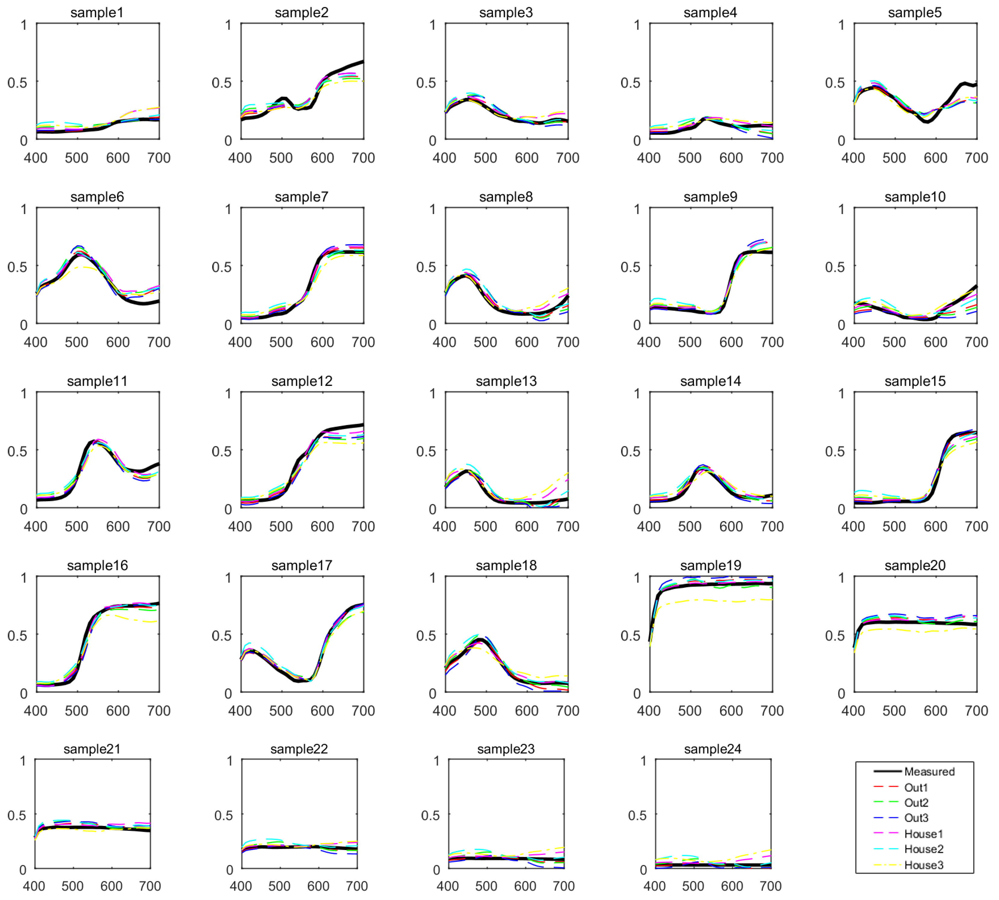
| Out1 | Out2 | Out3 | House1 | House2 | House3 | Average | |
|---|---|---|---|---|---|---|---|
| M1 | 3.51 | 4.32 | 4.55 | 4.05 | 5.06 | 6.11 | 4.60 |
| M1+M2 | 3.31 | 4.32 | 4.45 | 3.76 | 4.90 | 5.91 | 4.44 |
| MST++ | 10.66 | 13.45 | 12.47 | 11.07 | 8.97 | 8.43 | 10.84 |
| Out1 | Out2 | Out3 | House1 | House2 | House3 | Average | |
|---|---|---|---|---|---|---|---|
| M1 | 3.50 | 5.43 | 5.79 | 4.43 | 6.15 | 7.46 | 5.46 |
| M1+M2 | 4.01 | 6.60 | 6.40 | 3.87 | 7.13 | 6.57 | 5.76 |
| MST++ | 8.83 | 9.19 | 10.46 | 8.13 | 6.87 | 7.86 | 8.56 |
| Out1 | Out2 | Out3 | House1 | House2 | House3 | Average | |
|---|---|---|---|---|---|---|---|
| M1 | 5.70 | 7.36 | 9.18 | 7.03 | 7.52 | 9.30 | 7.68 |
| M1+M2 | 5.60 | 7.13 | 8.70 | 6.50 | 7.49 | 8.44 | 7.31 |
| MST++ | 9.11 | 12.74 | 9.10 | 8.26 | 7.99 | 8.87 | 9.35 |
| Out1 | Out2 | Out3 | House1 | House2 | House3 | Average | |
|---|---|---|---|---|---|---|---|
| M1 | 0.12 | 0.17 | 0.17 | 0.20 | 0.25 | 0.31 | 0.20 |
| M1+M2 | 0.11 | 0.17 | 0.16 | 0.18 | 0.23 | 0.29 | 0.19 |
| MST++ | 0.43 | 0.38 | 0.52 | 0.34 | 0.25 | 0.29 | 0.37 |
| n | 1 | 3 | 5 | 10 | 20 | 30 | 40 | 50 |
|---|---|---|---|---|---|---|---|---|
| CCSG | 2.50 | 2.58 | 2.59 | 2.60 | 2.59 | 2.60 | 2.59 | 2.59 |
| Munsell | 1.60 | 1.66 | 1.67 | 1.67 | 1.66 | 1.67 | 1.66 | 1.66 |
| Pigment | 2.90 | 2.99 | 2.99 | 3.00 | 3.00 | 3.00 | 3.02 | 3.00 |
| Out1 | 3.60 | 3.64 | 3.62 | 3.50 | 3.40 | 3.35 | 3.31 | 3.33 |
| Out2 | 4.38 | 4.30 | 4.23 | 4.25 | 4.42 | 4.37 | 4.32 | 4.32 |
| Out3 | 4.81 | 4.48 | 4.59 | 4.65 | 4.66 | 4.52 | 4.45 | 4.39 |
| House1 | 4.54 | 4.57 | 4.58 | 4.54 | 4.40 | 4.03 | 3.76 | 3.70 |
| House2 | 4.95 | 4.95 | 4.94 | 4.88 | 4.90 | 4.88 | 4.90 | 4.91 |
| House3 | 5.88 | 5.90 | 5.93 | 5.91 | 5.92 | 5.91 | 5.91 | 5.90 |
| n | 1 | 3 | 5 | 10 | 20 | 30 | 40 | 50 |
|---|---|---|---|---|---|---|---|---|
| CCSG | 1.38 | 1.65 | 1.65 | 1.70 | 1.69 | 1.07 | 1.69 | 1.70 |
| Munsell | 1.01 | 1.32 | 1.34 | 1.38 | 1.34 | 1.33 | 1.33 | 1.33 |
| Pigment | 1.26 | 1.62 | 1.64 | 1.64 | 1.59 | 1.59 | 1.61 | 1.60 |
| Out1 | 4.44 | 4.56 | 4.48 | 4.35 | 4.25 | 4.14 | 4.01 | 4.10 |
| Out2 | 6.96 | 6.78 | 6.59 | 6.66 | 7.00 | 6.81 | 6.60 | 6.65 |
| Out3 | 7.11 | 6.24 | 6.59 | 6.80 | 6.83 | 6.45 | 6.40 | 6.35 |
| House1 | 5.18 | 5.22 | 5.23 | 5.19 | 4.98 | 4.37 | 3.87 | 3.65 |
| House2 | 7.37 | 7.33 | 7.29 | 7.14 | 7.17 | 7.12 | 7.13 | 7.12 |
| House3 | 6.89 | 6.94 | 6.81 | 6.78 | 6.82 | 6.68 | 6.57 | 6.44 |
Disclaimer/Publisher’s Note: The statements, opinions and data contained in all publications are solely those of the individual author(s) and contributor(s) and not of MDPI and/or the editor(s). MDPI and/or the editor(s) disclaim responsibility for any injury to people or property resulting from any ideas, methods, instructions or products referred to in the content. |
© 2025 by the authors. Licensee MDPI, Basel, Switzerland. This article is an open access article distributed under the terms and conditions of the Creative Commons Attribution (CC BY) license (https://creativecommons.org/licenses/by/4.0/).
Share and Cite
Liang, J.; Hu, X.; Li, Y.; Xiao, K. Multispectral Reconstruction in Open Environments Based on Image Color Correction. Electronics 2025, 14, 2632. https://doi.org/10.3390/electronics14132632
Liang J, Hu X, Li Y, Xiao K. Multispectral Reconstruction in Open Environments Based on Image Color Correction. Electronics. 2025; 14(13):2632. https://doi.org/10.3390/electronics14132632
Chicago/Turabian StyleLiang, Jinxing, Xin Hu, Yifan Li, and Kaida Xiao. 2025. "Multispectral Reconstruction in Open Environments Based on Image Color Correction" Electronics 14, no. 13: 2632. https://doi.org/10.3390/electronics14132632
APA StyleLiang, J., Hu, X., Li, Y., & Xiao, K. (2025). Multispectral Reconstruction in Open Environments Based on Image Color Correction. Electronics, 14(13), 2632. https://doi.org/10.3390/electronics14132632