Filter-Based Tchebichef Moment Analysis for Whole Slide Image Reconstruction

Abstract

In digital pathology, accurate diagnosis and prognosis critically depend on robust feature representation of Whole Slide Images (WSIs). While deep learning offers powerful solutions, its “black box” nature presents significant challenges to clinical interpretability and widespread adoption. Handcrafted features offer interpretability, yet orthogonal moments, particularly Tchebichef moments (TMs), remain underexplored for WSI analysis. This study introduces TMs as interpretable, efficient, and scalable handcrafted descriptors for WSIs, alongside a novel two-dimensional digital filter architecture designed to enhance numerical stability and hardware compatibility during TM computation. We conducted a comprehensive reconstruction analysis using H&E-stained WSIs from the MIDOG++ dataset to evaluate TM effectiveness. Our results demonstrate that lower-order TMs accurately reconstruct both square and rectangular WSI patches, with performance stabilising beyond a threshold moment order, confirmed by SNIRE, SSIM, and BRISQUE metrics, highlighting their capacity to retain structural fidelity. Furthermore, our analysis reveals significant computational efficiency gains through the use of pre-computed polynomials. These findings establish TMs as highly promising, interpretable, and scalable feature descriptors, offering a robust alternative for computational pathology applications that prioritise both accuracy and transparency.

1. Introduction

Whole Slide Images (WSIs) have revolutionised the field of pathology by enabling the high-resolution digitisation of histopathological slides, thereby facilitating remote diagnostics, quantitative analysis, and AI-assisted decision support [1]. This technological advancement has catalysed substantial progress in digital and computational pathology, supporting applications such as automated disease classification, biomarker discovery, and prognosis prediction [2,3]. Despite significant advances in deep learning methodologies, several recent studies continue to underscore the relevance of handcrafted features within computational pathology.

Interpretability and expandability are critical considerations for the clinical adoption of AI in pathology. Despite the impressive performance, deep learning-based algorithms often operate as “black boxes,” providing little insight into how decisions are made [4]. This lack of transparency poses a significant barrier to trust and acceptance in clinical settings, where explainability is essential for validation and regulatory approval [5]. Although recent advancements in explainable AI, including attention mechanisms, saliency maps, and graph-based neural networks, have enhanced our understanding of the internal workings of deep models [6,7,8], these methods often provide only partial explanations or are difficult to interpret consistently across cases. As a result, there remains a pressing need for complementary or alternative approaches that prioritise transparency, reproducibility, and alignment with domain expertise.

Handcrafted pathological features are extracted from images using traditional image processing techniques, frequently guided by the expertise of trained pathologists [9]. These features offer enhanced interpretability. These features are designed to quantify the morphological structures, texture patterns, and spatial relationships discernible in WSIs. In contrast, deep features are representations automatically learned by deep learning algorithms. While such features can capture complex, hierarchical information and achieve performance levels comparable to those of expert pathologists, their application does not invariably guarantee superior accuracy across all computational pathology tasks.

Alhindi et al. [10] evaluated the relative efficacy of handcrafted versus deep features for the classification of malignant and benign tissue samples. Their results indicated that handcrafted features achieved higher classification accuracy, thereby suggesting their superior utility in certain tasks. More recently, Bolus Al Baqain and Sultan Al-Kadi [11] reported that handcrafted features tend to outperform in classification tasks, whereas deep features are generally more effective in segmentation applications. Furthermore, Huang et al. [12] proposed a hybrid framework that integrates both handcrafted and deep features, demonstrating improved classification performance in computational pathology.

Despite extensive exploration of handcrafted descriptors such as Local Binary Patterns (LBPs), Histogram of Oriented Gradients (HOG), Speeded-Up Robust Features (SURFs), and Scale-Invariant Feature Transform (SIFT), there remains a paucity of research investigating the use of image orthogonal moments as feature descriptors in WSIs. Orthogonal moments, such as Zernike [13], Legendre [14], and Chebyshev [15], are mathematical descriptors that provide compact yet accurate representations of image structures and have proven valuable in numerous image analysis tasks, including biomedical imaging [16]. Among these, Tchebichef Moments (TMs) are particularly notable for their discrete orthogonality, which facilitates superior image reconstruction without reliance on continuous-domain approximations [17,18].

TMs have demonstrated the ability to achieve high-fidelity image representation with minimal redundancy, and have been successfully applied in domains such as satellite imaging [19] and medical image analysis [20,21]. In computational pathology, TMs have previously been utilised to extract textural features for the classification of colorectal cancer [22]. While these findings underscore the potential of TMs as effective feature descriptors, the aforementioned study was limited in scope, having relied solely on the red channel of WSIs, thereby constraining its utility as a full RGB feature descriptor.

In the present study, we propose a two-dimensional cascaded digital filter architecture for the efficient and accurate generation of TMs, specifically tailored for WSI reconstruction. Additionally, we conduct a comprehensive reconstruction analysis of WSIs to assess the capacity of TMs to capture salient features. This research aims to address the gap in the current literature by demonstrating the utility of Tchebichef moments as robust and interpretable feature descriptors in computational pathology.

This paper is organised as follows. Section 1 introduces the background of WSIs, the challenges in digital pathology, and the motivation for using TMs as interpretable feature descriptors. Section 2 presents the theoretical foundations of Tchebichef Polynomials and Moments, including their mathematical definitions and properties, and discusses their application to coloured images. Section 3 details the proposed novel filter structure designed for the efficient computation of Tchebichef polynomials. Section 4 provides the experimental results and discussion, covering the dataset used, algorithm implementation, reconstruction analysis, and evaluation of time complexity. Concluding remarks and future work are presented in Section 5.

2. Mathematical Background

In this section, we define the 2D TM for image analysis using orthogonal discrete Tchebichef polynomials $t_p\left(n\right)$, specifying the norm function $\rho (p,N)$ and normalisation factor $\beta (p,N)$, along with their recurrence relation, and detailing how images can be reconstructed from TMs and how polynomials are represented. We then extend TMs to colour images, noting the limitations of greyscale approaches and introducing channel-wise TM computation for red, green, and blue components, culminating in the introduction of Quaternion Tchebichef Moments (QTMs) for a more integrated representation using quaternion algebra.

2.1. Tchebichef Polynomials and Moments

The 2D Tchebichef moment of order $(p+q)$ for an image intensity function $f(n,m)$, with dimensions $N\times M$, is defined as

$$T_{pq}=A(p,N)A(q,M)\sum _{n=0}^{N-1}\sum _{m=0}^{M-1}{t}_p\left(n\right)t_q\left(m\right)f(n,m),$$

(1)

where $t_p\left(n\right)$ denotes the orthogonal discrete Tchebichef polynomial of order p, as given by Mukundan et al. [17]:

$$t_p\left(n\right)=p!\sum _{k=0}^p{(-1)}^{p-k}\left({\displaystyle \genfrac{}{}{0pt}{}{N-1-k}{p-k}}\right)\left({\displaystyle \genfrac{}{}{0pt}{}{p+k}{p}}\right)\left({\displaystyle \genfrac{}{}{0pt}{}{n}{k}}\right).$$

(2)

Additionally, the coefficient $A(p,N)$ is defined as

$$A(p,N)={\displaystyle \frac{\beta (p,N)}{\rho (p,N)}},$$

where $\beta (p,N)$ serves as a normalisation factor, typically chosen as $N^p$. Furthermore, the orthogonality of the polynomials is governed by the squared norm

$$\rho (p,N)=\left(2p\right)!\left({\displaystyle \genfrac{}{}{0pt}{}{N+p}{2p+1}}\right).$$

The recurrence relation for the Tchebichef polynomials is expressed as

$$(p+1)t_{p+1}\left(n\right)-(2p+1)(2n-N+1)t_p\left(n\right)+p(N^2-p^2)t_{p-1}\left(n\right)=0,$$

(3)

for $p\ge 1$, with the initial polynomials given by $t_0\left(n\right)=1$ and $t_1\left(n\right)=2n-N+1$.

As shown in Figure 1, the top panel presents a plot of discrete Tchebichef polynomial values for $N=8$. Complementing this, the bottom panel displays an $8\times 8$ array of basis images for the two-dimensional discrete Tchebichef transform.

Given a set of TMs up to order $(N_{\max },M_{\max })$, the image function $f(n,m)$ can be approximated by the reconstruction formula

$$\tilde{f}(n,m)=\sum _{p=0}^{N_{\max }}\sum _{q=0}^{M_{\max }}{\displaystyle \frac{1}{\beta (p,N)\beta (q,M)}}{T}_{pq}{t}_p\left(n\right)t_q\left(m\right).$$

(4)

The discrete Tchebichef polynomial $t_p\left(n\right)$ may also be represented as a polynomial in n, as reported by Mukundan et al. [17]:

$$t_p\left(n\right)=\sum _{k=0}^n{C}_k(p,N)\sum _{i=0}^k{s}_k^{\left(i\right)}{n}^i,$$

(5)

where $C_k(p,N)={(-1)}^{p-k}{\displaystyle \frac{p!}{k!}}\left({\displaystyle \genfrac{}{}{0pt}{}{N-1-k}{p-k}}\right)\left({\displaystyle \genfrac{}{}{0pt}{}{p+k}{p}}\right)$, and $s_k^{\left(i\right)}$ are the Stirling numbers of the first kind [23], satisfying the identity ${\displaystyle \frac{x!}{(x-k)!}}={\sum }_{i=0}^k{s}_k^{\left(i\right)}{x}^i.$

2.2. Tchebichef Moments in Coloured Image

To this day, most studies involving TMs have been conducted on greyscale images or rely on a single colour channel. This approach helps reduce computational cost and is generally sufficient for applications such as shape analysis, watermarking, texture classification, and image retrieval, where greyscale representations adequately capture the relevant features [24,25,26,27]. However, in digital pathology, the colour information in histological slides is critical for accurate analysis. Converting WSIs to greyscale in this context can result in significant information loss, potentially compromising diagnostic accuracy [28].

While greyscale representations are commonly used in image analysis with TMs, the method is not inherently limited to greyscale and can be effectively extended to colour images using techniques such as channel-wise computation or quaternion-based formulations. The most straightforward approach is channel-wise computation, where TMs are calculated separately for each colour channel. This allows for the independent extraction of structural features from the red, green, and blue channels, resulting in three distinct sets of 2D Tchebichef moments per image:

$$f(x,y)=\{f_{\mathrm{R}}(x,y),f_{\mathrm{G}}(x,y),f_{\mathrm{B}}(x,y)\}\Rightarrow \{T{M}_{\mathrm{R}},T{M}_{\mathrm{G}},T{M}_{\mathrm{B}}\},$$

where $f(x,y)$ is the image function represented as a set of RGB intensity functions, and $T{M}_{\mathrm{R}},T{M}_{\mathrm{G}},T{M}_{\mathrm{B}}$ denote the corresponding TMs computed separately for the red, green, and blue channels, respectively.

Recently, QTMs proposed by Zhu et al. [29] have gained increasing attention for coloured image analysis. These QTMs compute the TMs for colored images by integrating quaternion algebra, which inherently models the correlation between different colour channels. An RGB image can be expressed as a quaternion vector as follows:

$$f(x,y)=f_{\mathrm{R}}(x,y)\mathbf{i}+f_{\mathrm{B}}(x,y)\mathbf{j}+f_{\mathrm{B}}(x,y)\mathbf{k}.$$

Using the quaternion vector of the image, the QTMs of a square image with a quaternion root of $-1$ can be computed as shown:

$$\begin{array}{cc}\hfill QT{M}_{pq}& =-\sum _{x=0}^{N-1}\sum _{y=0}^{N-1}{\displaystyle \frac{\left(f_{\mathrm{R}}(x,y)\mathbf{i}+f_{\mathrm{G}}(x,y)\mathbf{j}+f_{\mathrm{B}}(x,y)\mathbf{k}\right)t_p\left(x\right)t_q\left(y\right)(\mathbf{i}+\mathbf{j}+\mathbf{k})}{\sqrt{3}}}\hfill \\ \hfill & ={\displaystyle \frac{1}{\sqrt{3}}}\left[\sum _{x=0}^{N-1}\sum _{y=0}^{N-1}\left(f_{\mathrm{R}}(x,y)+f_{\mathrm{G}}(x,y)+f_{\mathrm{B}}(x,y)\right)t_p\left(x\right)t_q\left(y\right)\right]\hfill \\ \hfill & -\mathbf{i}{\displaystyle \frac{1}{\sqrt{3}}}\left[\sum _{x=0}^{N-1}\sum _{y=0}^{N-1}\left(f_{\mathrm{G}}(x,y)-f_{\mathrm{B}}(x,y)\right)t_p\left(x\right)t_q\left(y\right)\right]\hfill \\ \hfill & -\mathbf{j}{\displaystyle \frac{1}{\sqrt{3}}}\left[\sum _{x=0}^{N-1}\sum _{y=0}^{N-1}\left(f_{\mathrm{B}}(x,y)-f_{\mathrm{R}}(x,y)\right)t_p\left(x\right)t_q\left(y\right)\right]\hfill \\ \hfill & -\mathbf{k}{\displaystyle \frac{1}{\sqrt{3}}}\left[\sum _{x=0}^{N-1}\sum _{y=0}^{N-1}\left(f_{\mathrm{R}}(x,y)-f_{\mathrm{G}}(x,y)\right)t_p\left(x\right)t_q\left(y\right)\right]\hfill \\ \hfill & =A_0+\mathbf{i}{A}_1+\mathbf{j}{A}_2+\mathbf{k}{A}_3,\hfill \end{array}$$

(6)

where

$$A_0={\displaystyle \frac{1}{\sqrt{3}}}\left[T{M}_{\mathrm{R}}+T{M}_{\mathrm{G}}+T{M}_{\mathrm{B}}\right],A_1=-{\displaystyle \frac{1}{\sqrt{3}}}\left[T{M}_{\mathrm{G}}-T{M}_{\mathrm{B}}\right],$$

$$A_2=-{\displaystyle \frac{1}{\sqrt{3}}}\left[T{M}_{\mathrm{B}}-T{M}_{\mathrm{R}}\right],\mathrm{and}{A}_3=-{\displaystyle \frac{1}{\sqrt{3}}}\left[T{M}_{\mathrm{R}}-T{M}_{\mathrm{G}}\right].$$

The QTMs use channel-wise computation to derive Tchebichef moments for each RGB channel. These moments are then combined into a single quaternion representation that preserves both spatial and colour information.

In 2020, Elouariachi et al. [30] introduced QTMs with invariance to rotation, scale, and translation, making them particularly suitable for robust pattern recognition and image classification tasks. In their study, the proposed QTM invariants were successfully applied to hand gesture recognition. Subsequently, QTMs have been integrated with deep learning frameworks to achieve accurate classification of natural images [31] and for facial recognition [32]. In both studies, modified neural network architectures were proposed to accept QTMs as input data. While this approach has shown promising results, the quaternion vector is not a conventional input format for deep learning models, which may introduce challenges during implementation.

3. Proposed Filter Structure

We introduce a novel formula for the efficient computation of Tchebichef polynomials. By employing the backwards difference technique, we obtain a simplified input for the designed filter across any arbitrary order, making it independent of the image size (N). To further enhance efficiency, we implement a cascaded digital filter structure, leveraging the following lemma and theorem.

Lemma 1.

Let $Q_p\left(n\right)$ be a polynomial of degree $p\ge 1$, expressed as $Q_p\left(n\right)=a{n}^p+b{n}^{p-1}+l.o.t.$ where $a\ne 0,b$ are real coefficients, and l.o.t. represents lower-order terms (if any). Applying the $p^{th}$-order backwards difference operator ${\nabla }^p$ to $Q_p\left(n\right)$ results in

$${\nabla }^n\left\{Q_p\left(n\right)\right\}=ap!,$$

(7)

and ∇ represents the backwards difference operator, defined as $\nabla f\left(n\right)=f\left(n\right)-f(n-1)$. This shows that only the coefficient of the highest-order term remains (leading coefficient) while any further backwards differences yield zero, as the result is constant with respect to n.

Proof. 

The proof follows directly by induction and is straightforward to verify (for further details, please refer to the inductive proof in [33]).    □

Compared to forward and central difference operators, the backwards difference operator offers two key advantages in our context. First, it simplifies the derivation of the factorial-scaled leading coefficient when applied to a polynomial of matching order. Second, it is inherently causal, making it well-suited for hardware-oriented implementations such as Field-Programmable Gate Array (FPGA)-based systems. In contrast, central differences require access to future values and introduce symmetry-related constraints, while forward differences can complicate boundary handling in convolutional architectures. Therefore, the backwards difference operator provides both theoretical clarity and practical efficiency for moment-based digital filtering.

Theorem 1.

The discrete Tchebichef polynomials satisfy the following property:

$${\nabla }^p\left\{t_p\left(n\right)\right\}={\displaystyle \frac{\left(2p\right)!}{p!}},$$

(8)

where p denotes the polynomial order.

Proof. 

Using Equation (5), the leading coefficient of $n^p$ in $t_p\left(n\right)$ arises from the term where $k=p$ and $i=p$. Since $s_p^{\left(p\right)}=1$ and $s_k^{\left(i\right)}=0$ for $i>k$, the leading coefficient of $t_p\left(n\right)$ is $C_p(p,N)s_p^{\left(p\right)}=C_p(p,N)$. Substituting $k=p$ into the expression for $C_k(p,N)$ :

$$C_p(p,N)={(-1)}^{p-p}{\displaystyle \frac{p!}{p!}}\left({\displaystyle \genfrac{}{}{0pt}{}{N-1-p}{p-p}}\right)\left({\displaystyle \genfrac{}{}{0pt}{}{p+p}{p}}\right)=\left(1\right)\left(1\right)\left(1\right)\left({\displaystyle \genfrac{}{}{0pt}{}{2p}{p}}\right)=\left({\displaystyle \genfrac{}{}{0pt}{}{2p}{p}}\right),$$

Thus, the leading coefficient of $t_p\left(n\right)$ is $\left({\displaystyle \genfrac{}{}{0pt}{}{2p}{p}}\right)$. Utilising lemma 1, the p-th order backwards difference of the Tchebichef polynomials is given by $\left({\displaystyle \genfrac{}{}{0pt}{}{2p}{p}}\right)p!$, which further simplifies to ${\displaystyle \frac{\left(2p\right)!}{p!}}$ and concludes the proof.    □

By applying the flipped version of the input WSI image to our designed filter structure, we can compute TMs of arbitrary orders. Based on the findings in [34], a discrete transformation of a discrete signal $f\left(n\right)$ of length N over a kernel function $g(n,p)$ can be obtained through the discrete convolution of the kernel with the flipped signal, evaluated at $N-1$. It means

$$T_{pq}=\sum _{n=0}^{N-1}\sum _{m=0}^{M-1}f(n,m)t_p\left(n\right)t_q\left(m\right)=f^F(n,m)\ast t_p\left(n\right)t_q\left(m\right){|}_{n=N-1,m=M-1},$$

(9)

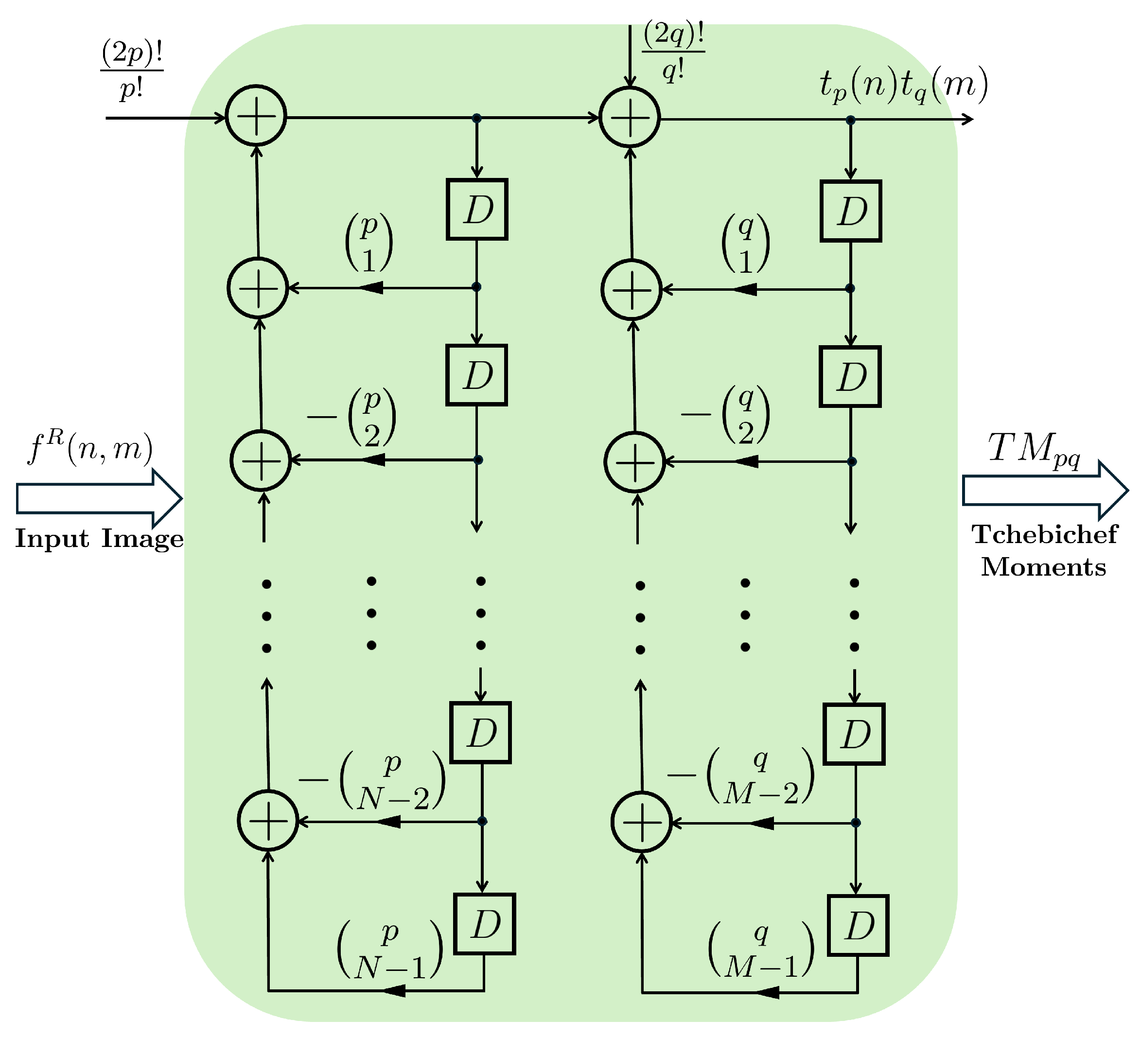
where * is 2D convolution and $f^F(n,m)$ represents the flipped WSI image. Figure 2 illustrates the structure of a cascaded digital filter based on successive backwards differences including $(N+M-2)$ delay blocks and $(N+M-2)$ binomial terms of $\pm \left({\displaystyle \genfrac{}{}{0pt}{}{p}{i}}\right)$ and $\pm \left({\displaystyle \genfrac{}{}{0pt}{}{q}{j}}\right)$ (where $i=1,2,\dots ,N-1$ and $j=1,2,\dots ,M-1$) are multipliers to show the specific order of the polynomial.

Figure 3 presents a flowchart of the proposed algorithm for computing and reconstructing WSIs using TMs. It begins with a WSI input, followed by TM calculation using weighted pixel sums. A cascaded digital filter accelerates this process. The reconstructed image is obtained using the TMs features and Tchebichef kernels. Image quality assessment (IQA) includes Blind/Referenceless Image Spatial Quality Evaluator (BRISQUE) as a no-reference score and Statistical Normalisation Image Reconstruction Error (SNIRE)/Structural Similarity Index Measure (SSIM) as full-reference scores. This workflow highlights the effectiveness of TMs in image processing and evaluation.

4. Experimental Results and Discussion

An experimental study was conducted to evaluate the effectiveness of TMs as feature representations for WSI reconstruction in histopathology analysis. As outlined in the previous section, we proposed a novel two-dimensional filter architecture designed to provide a theoretically efficient and mathematically elegant framework for TMs computation, with potential benefits in numerical precision and hardware compatibility. However, given that the primary objective of this study is to assess the utility of TMs in WSI reconstruction, we employed a validated and computationally efficient C++ implementation for all experimental analyses. This decision ensured consistency, scalability, and robustness when processing large-scale WSIs. The proposed filter is therefore presented as a theoretical contribution, with plans for future work to benchmark its performance, optimise its implementation, and explore its applicability in real-time or resource-constrained environments.

4.1. Data

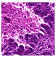
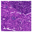
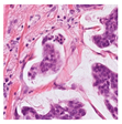
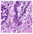
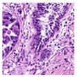
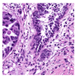
For the reconstruction analysis, Hematoxylin and Eosin (H&E)-stained WSIs from the MIDOG++ dataset [35] were utilised due to the dataset’s diversity in tumour types and morphological characteristics. The dataset consists of 503 WSIs containing mitotic figures from seven tumour types collected from both human and canine specimens: breast carcinoma, neuroendocrine tumour, lung carcinoma, lymphosarcoma, cutaneous mast cell tumour, melanoma, and soft tissue sarcoma. Sample WSIs from the dataset are illustrated in Figure 4. To evaluate the capability of TMs in capturing spatial and structural information, WSIs were cropped into patches of varying sizes, enabling assessment of TM sensitivity to image scale and feature size. Additionally, the dataset’s physiological and staining variability provided a means to test the robustness of TMs in encoding visual features from diverse WSIs. The WSIs were cropped into patches of varying dimensions.

4.2. Algorithm Implementation

High-order Tchebichef polynomials and moments are prone to numerical instability, particularly when applied to large-scale image data, which can result in inaccurate reconstructions. To address this, several algorithms have been developed to enable stable and precise computation of these polynomials. In this study, we implemented the method proposed by Camacho-Bello and Rivera-Lopez [36] in C++ for the efficient computation of TMs on large WSIs. This approach incorporates the recurrence relation introduced by Mukundan et al. [17] and applies the Gram–Schmidt orthonormalisation process to maintain numerical stability and accuracy at high polynomial orders.

The quality of WSI reconstruction was evaluated using three image quality metrics: SNIRE [18], SSIM [37], and BRISQUE [38]. SNIRE quantifies pixel-wise reconstruction error relative to the original image, while SSIM measures perceived similarity, where a value of 1 indicates perfect similarity and 0 indicates no similarity. BRISQUE evaluates the perceptual quality of an image without a reference, with lower scores indicating higher quality (0 being the best and 100 the worst). It is noteworthy that BRISQUE did not yield a score of 0 even for the original WSIs, likely due to its interpretation of histological textures as noise. Therefore, the BRISQUE score of the original WSI was used as a baseline for comparative analysis.

4.3. Reconstruction Analysis

In contrast to traditional handcrafted features such as LBP, HOG, SURF, and SIFT, TMs do not provide pixel-wise interpretability. Instead, they provide a powerful global representation of the image by encoding high-level characteristics, including texture, shape, colour, and spatial structure—features that are crucial for distinguishing between pathological and healthy tissues. While their interpretability may be limited at the level of specific diagnostic indicators, TMs enable reconstruction-based interpretability, allowing us to assess how well visual information is retained through the encoded moments.

In this paper, we conduct both qualitative and quantitative reconstruction analyses to evaluate the extent to which TMs preserve salient information from WSIs. It is important to clarify that the purpose of this analysis is not to assess the robustness of TMs to noise or artefacts, nor to benchmark their reconstruction fidelity against deep learning models such as autoencoders. Rather, the goal is to demonstrate that meaningful and diagnostically relevant visual information is effectively encoded by TMs across different moment orders.

Table 1. Reconstructed WSIs of dimensions $1000\times 1000$ with varying maximum reconstruction orders.

Original	Maximum Reconstruction Order
Image	50	100	200	400	800	1000
SNIRE SSIM BRISQUE	0.0106 0.3791 76.1671	0.0059 0.4711 61.6342	0.0025 0.6834 57.3636	0.0005 0.9346 42.0573	0.0 0.9966 35.6887	0.0 1.0 38.4073
SNIRE SSIM BRISQUE	0.0109 0.4754 78.4379	0.0046 0.6133 65.4458	0.0015 0.8075 55.1812	0.0002 0.9657 40.4472	0.0 0.9973 32.3747	0.0 1.0 34.0520
SNIRE SSIM BRISQUE	0.0425 0.2273 83.9600	0.0226 0.3809 67.2707	0.0102 0.6140 56.5922	0.0035 0.8625 35.9452	0.0002 0.9915 14.3345	0.0 1.0 13.0210
SNIRE SSIM BRISQUE	0.0254 0.3760 75.9400	0.0144 0.4845 55.0308	0.0076 0.6566 46.4713	0.0026 0.8783 37.6347	0.0002 0.9925 12.6129	0.0 1.0 21.5446

presents four randomly selected $1000\times 1000$ pixel patches extracted from WSIs in the MIDOG++ dataset, along with their respective reconstructions using TMs of varying orders. For comparison,

Table 2. Reconstructed natural images of dimensions $1000\times 1000$ with varying maximum reconstruction orders.

Original	Maximum Reconstruction Order
Image	50	100	200	400	800	1000
SNIRE SSIM BRISQUE	0.6768 0.3959 98.9336	0.6106 0.4299 79.7782	0.5383 0.5595 65.3323	0.3718 0.8481 48.8923	0.0157 0.9974 44.6995	0.0 1.0 44.7999
SNIRE SSIM BRISQUE	0.9394 0.3137 97.0276	0.8500 0.3825 76.7839	0.7469 0.5576 59.3039	0.5533 0.8217 39.1302	0.1064 0.9855 9.1570	0.0 1.0 7.8628
SNIRE SSIM BRISQUE	0.4384 0.7767 95.3218	0.2450 0.8388 82.1695	0.1384 0.8881 68.2615	0.0834 0.9355 47.7812	0.0192 0.9881 15.1678	0.0 1.0 11.6452
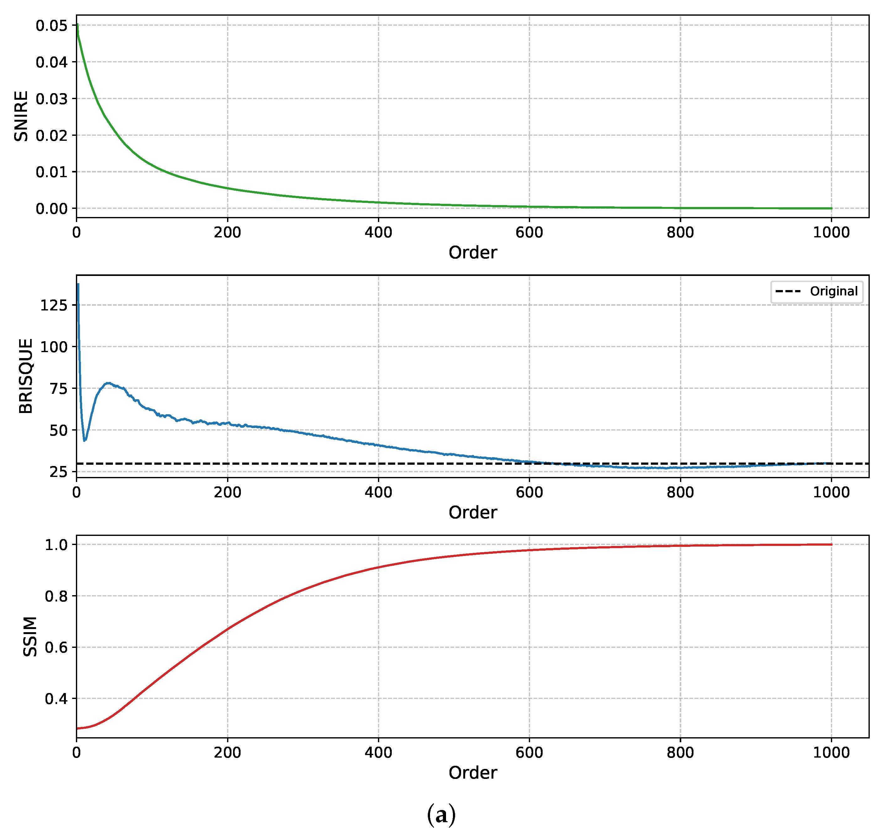
SNIRE SSIM BRISQUE	1.2027 0.1334 96.7264	1.1487 0.2032 74.2226	1.0583 0.4147 65.2873	0.8481 0.7871 44.1298	0.2612 0.9892 19.9911	0.0 1.0 16.5829

shows the reconstruction of natural images. The reconstructed WSIs exhibit a high degree of visual similarity to the originals, even at relatively low moment orders (e.g., order 50). By moment order 200, the reconstructions become visually indistinguishable from the original WSI to the human eye. In contrast, natural images require moment orders as high as 800 to achieve comparable visual fidelity. Furthermore, the variation in reconstruction quality across WSIs at a given order is smaller and more consistent than that observed in natural images, indicating that TMs encode features from WSIs more efficiently. These findings suggest that TMs are well-suited for capturing the semantic and structural characteristics of WSIs while maintaining reduced computational complexity. The ability to achieve high-fidelity reconstructions at lower moment orders underscores the potential of TMs as an efficient feature representation method in histopathological image analysis. Additional reconstruction results conducted using Python (version 3.13.2) are presented in Appendix A,highlighting that differences in computational environments and floating-point precision can affect the quality of the SNIRE.

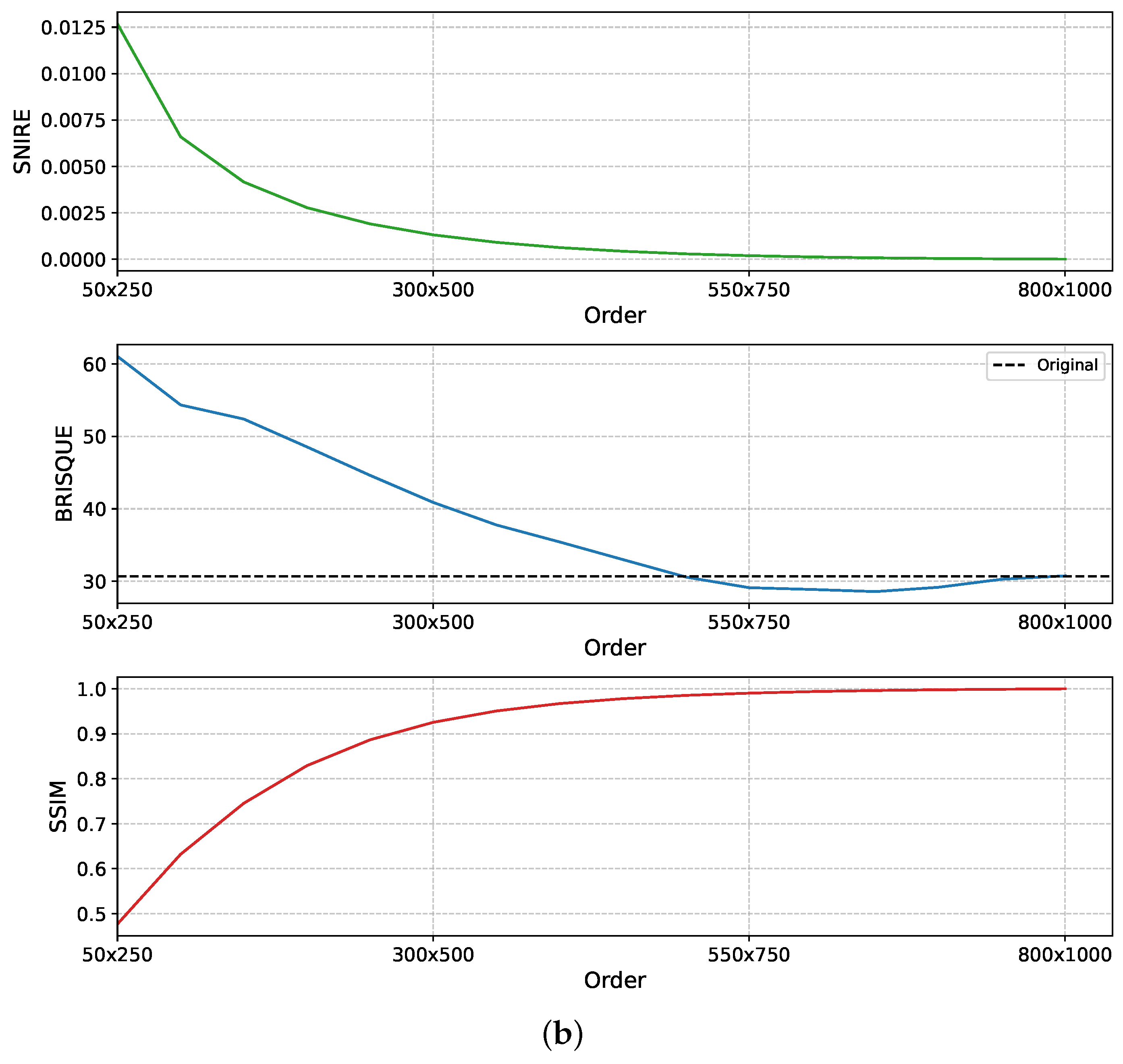
Further analysis in Figure 5, using both square (1000 × 1000) and rectangular (800 × 1000) WSI patches, shows that SNIRE, SSIM, and BRISQUE scores begin to stabilise at a maximum reconstruction order of 600 for square patches and around 550 × 750 for rectangular patches. This convergence indicates that increasing the moment order beyond this threshold yields diminishing returns in terms of reconstruction fidelity. Additionally, this demonstrates that TMs are effective not only for square patches, as commonly studied, but also for rectangular regions, thereby broadening their applicability in real-world WSI analysis. These findings support the argument that lower-order TMs are sufficient for accurate WSI reconstruction. These results further underscore the efficiency of TMs in capturing features within WSIs, highlighting their potential as effective handcrafted descriptors for digital pathology analysis.

Full reconstruction was performed on patches larger than 1000 pixels to demonstrate the capability of TMs in handling high-resolution images. Figure 6 and Figure 7 illustrate the successful reconstruction of large WSIs with dimensions up to $6000\times 5000$ pixels without any errors, underscoring the potential of TMs to efficiently process high-resolution data. This is particularly important in computational pathology, as it confirms that no numerical instability is introduced when handling large WSIs. Furthermore, since TMs effectively encode information even at lower moment orders, it is feasible to use only a subset of moments for analysis. This reduction in feature dimensionality presents a promising alternative to more computationally intensive methods. The ability to reconstruct WSIs using lower-order moments at reduced computational cost positions TMs as a valuable tool for large-scale computational pathology applications where both accuracy and efficiency are essential.

4.4. Redundancy and Dimensionality Analysis

In the reconstruction analysis, TMs demonstrated their ability to effectively and accurately encode visual semantic information from WSIs, achieving full reconstruction at the maximum moment order. As shown in the quantitative results in Figure 5, the quality of reconstructed images converges as the moment order increases, suggesting the presence of potentially redundant information at higher orders. To explore this, a redundancy analysis was conducted to assess whether high-order TMs introduce informational overlap. This analysis focused on square matrices for computational efficiency and interpretability, and employed both visual inspection of the correlation matrix and principal component analysis (PCA).

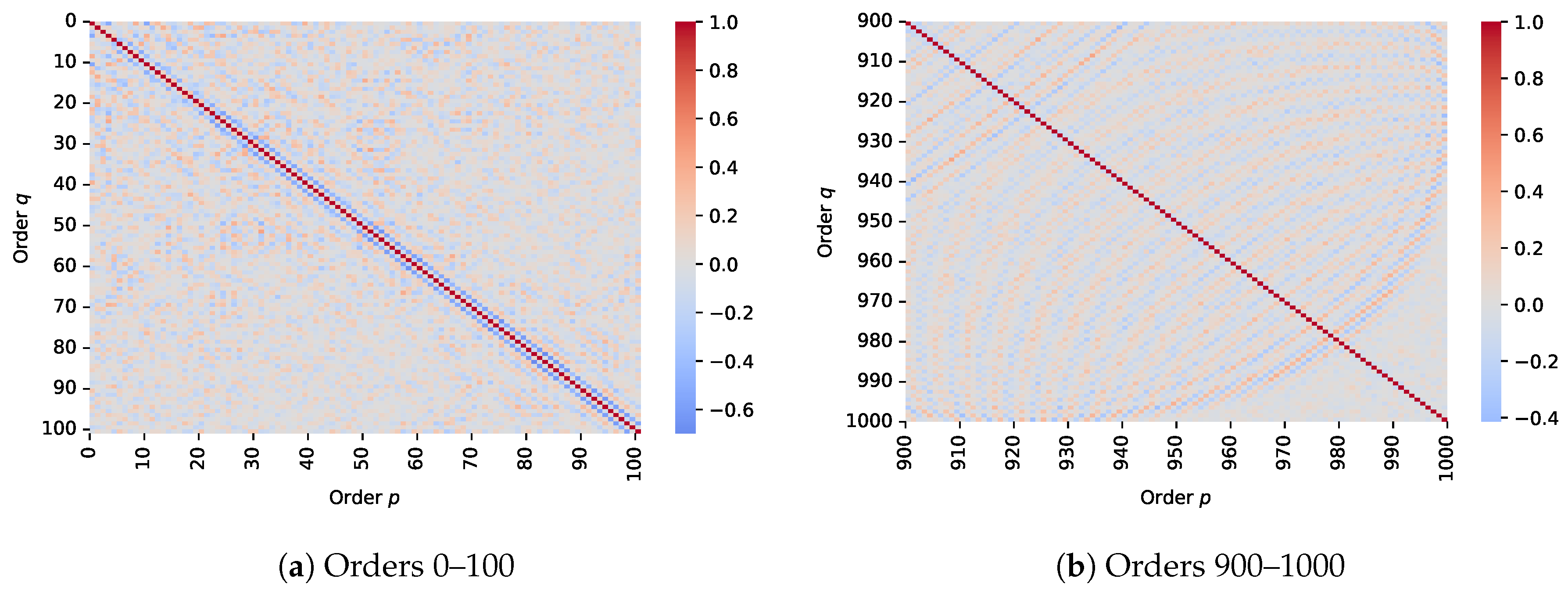
To analyse potential redundancy across moment orders, correlation matrices were visualised for two distinct subsets of TMs as shown in Figure 8: a lower-order range (1–100) and a higher-order range (901–1000). In the lower-order matrix, most off-diagonal values were near zero, indicating a weak correlation between moment pairs and suggesting a high degree of statistical independence. This supports the effectiveness of lower-order moments in capturing distinct and complementary image features. In contrast, the higher-order correlation matrix revealed pronounced diagonal bands which are perpendicular to the main diagonal, indicating a localised correlation between adjacent high-order moments. This pattern suggests increasing redundancy at higher orders, where moment values become more interdependent and potentially less informative.

These results align with the dimensionality analysis conducted via PCA, which similarly indicated that the majority of variance is captured by lower-order moments, as shown in Figure 9. An analysis of Tchebichef moments across a range of WSIs showed that a cumulative explained variance of 0.999 is achieved using moments of the order less than 200. The observed redundancy among higher-order moments, as revealed in the correlation matrix, corresponds to their diminishing contribution in PCA, reinforcing the conclusion that high-order moments provide limited additional information. Therefore, for image analysis tasks, features encoded at lower orders may be sufficient. This reduction not only preserves the essential information but also significantly lowers the computational burden of processing large WSIs, as the input feature space can be limited to a smaller subset of moment orders. The optimal moment order for feature extraction may vary depending on the specific task; therefore, further optimisation and careful selection of the appropriate moment order are recommended, particularly when applying TMs to classification or segmentation tasks.

4.5. Time Complexity

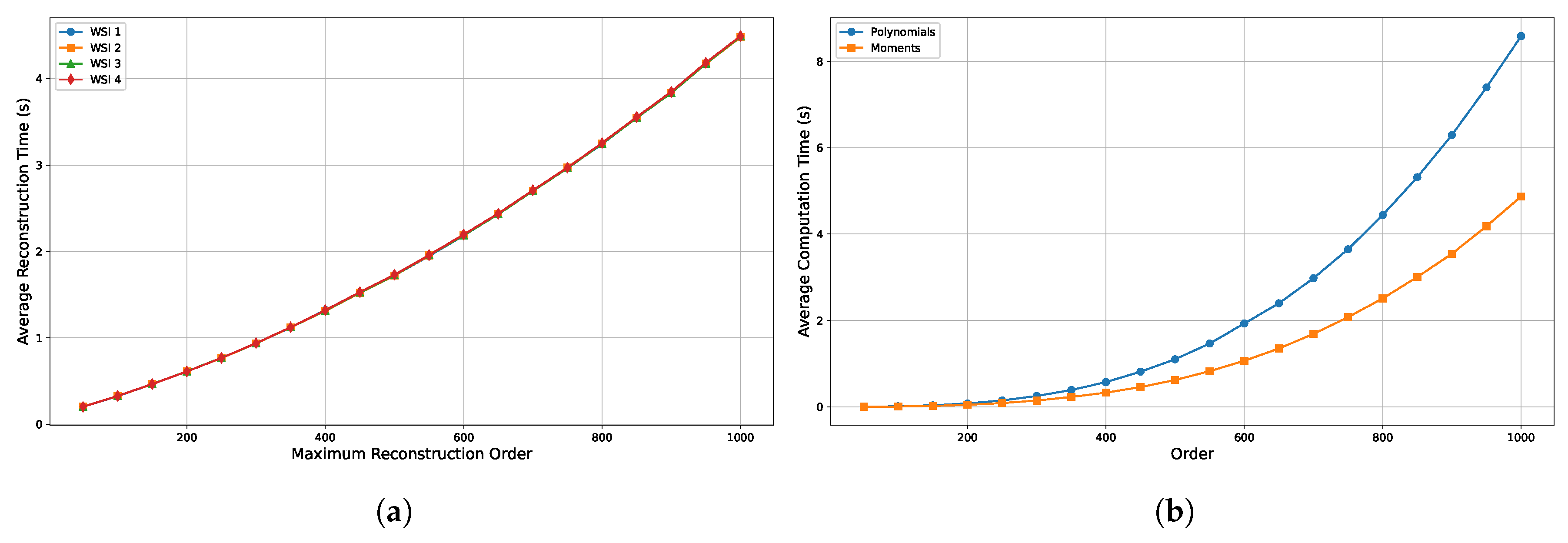
The time complexity of the Tchebichef polynomial generation, moment computation, and image reconstruction was measured on a CPU using a 12th Gen Intel® Core™ i7-12700F processor (Santa Clara, CA, USA) (2.19 GHz) with 64 GB of RAM. Figure 10a presents the average reconstruction time across varying maximum reconstruction orders, illustrating a time complexity of approximately $O(nlogn)$. This results in an increased computational cost as the order rises. Notably, the plot shows overlapping curves for different images, suggesting that the computation time is largely dominated by the reconstruction order rather than the image content itself. Although minor variations exist, they are negligible in scale, indicating that the reconstruction time is relatively consistent across different images. This implies that the computational burden is primarily a function of algorithmic complexity rather than specific image characteristics.

Figure 10b illustrates the computation times for Tchebichef polynomials and their corresponding moments across different orders. Polynomial computation exhibits a time complexity of $O\left(n^3\right)$, while moment computation requires $O\left(n^2\right)$. As a result, calculating polynomials and moments for every image can be computationally inefficient. This cost can be mitigated by using pre-computed Tchebichef polynomials, which remain constant for a given order and resolution. Since the polynomial dimensions depend on image resolution, bases for commonly encountered sizes (e.g., 32, 64, 128, 256, 512, 1024, and 2048) can be pre-computed and stored in binary or CSV format. These can then be loaded at runtime as needed, allowing for reuse across multiple images, eliminating redundant computations, and significantly improving overall efficiency.

However, despite utilising pre-computed polynomials, the computational complexity of moment calculation remains at $O\left(n^2\right)$, which may hinder real-time processing of high-resolution WSIs. Since all experiments in this study were conducted on a CPU, neither GPU acceleration nor multi-threaded parallel processing was explored. Given that the computation of moments involves repeated matrix operations, it lends itself well to parallelisation, which could significantly reduce runtime and enable real-time performance. Furthermore, implementing the proposed filter design on FPGAs or Application-Specific Integrated Circuits (ASICs) platforms could offer additional improvements in computational efficiency through hardware-level parallelism.

4.6. Integration with Machine and Deep Learning

Through the reconstruction analysis, we highlighted the efficiency of TMs and their ability to accurately encode high-level semantic and structural information from WSIs, while our redundancy analysis further demonstrated that lower-order subsets of TMs are more suitable for image analysis, as higher-order moments often carry redundant or less salient information. For integration into machine learning or deep learning pipelines, a selected subset of moments can be used as input features, as described in [16]. Alternatively, the full set of TMs can be concatenated with deep features to enhance representation, as explored in [39]. This can be achieved either by computing the full set of moments and identifying the optimal order during feature engineering, or by directly limiting the computation to a predefined moment order based on the task requirements.

5. Conclusions

This study introduced a novel two-dimensional cascaded digital filter architecture for the efficient computation of TMs and demonstrated its ability to encode visual features for digital pathology. Through extensive experiments using the MIDOG++ dataset, we showed that lower-order TMs can faithfully reconstruct diagnostically relevant WSI patches, with image quality metrics such as SSIM, SNIRE, and BRISQUE confirming their ability to retain structural and perceptual fidelity. Additionally, our redundancy and dimensionality analyses revealed that most of the informative content is encoded within lower-order moments, highlighting the efficiency and compactness of TMs as handcrafted descriptors.

Unlike traditional handcrafted features, which often offer pixel-wise interpretability, TMs enable reconstruction-based interpretability, allowing practitioners to visually assess the fidelity of encoded features. This property makes them especially valuable in clinical applications where transparency and interpretability are essential, providing image-level insight into what the model has learned, bridging the gap between abstract feature representations and human-understandable patterns.

The proposed filter architecture, while grounded in rigorous theoretical derivations, has not yet been benchmarked in practical hardware settings. Future work will focus on implementing this architecture on parallel hardware platforms, such as FPGAs and ASICs, which are well-suited for the cascaded and recursive structure of the design. Such platforms offer potential for achieving real-time performance even when processing high-resolution WSIs.

To support deployment in real-world diagnostic scenarios, particularly in edge-computing and resource-constrained environments, several optimisation strategies will be pursued. These include dynamic truncation of the maximum moment order based on task-specific accuracy requirements, thereby enabling a flexible balance between computational complexity and reconstruction quality. Additionally, memory-efficient schemes for storing and retrieving pre-computed Tchebichef polynomials will be explored, such as lookup tables or embedded ROM-based architectures, which can significantly reduce runtime and energy consumption.

Overall, this research establishes Tchebichef Moments as robust, interpretable, and scalable feature descriptors for computational pathology and lays the foundation for further advancements in real-time and embedded WSI analysis systems.