A Remote Sensing Image Object Detection Model Based on Improved YOLOv11

Abstract

Due to the challenges posed by high resolution, substantial background noise, significant object scale variation, and long-tailed data distribution in remote sensing images, traditional techniques often struggle to maintain both high accuracy and low latency. This paper proposes YOLO11-FSDAT, an advanced object detection framework tailored for remote sensing imagery, which integrates not only modular enhancements but also theoretical and architectural innovations to address these limitations. First, we propose the frequency–spatial feature extraction fusion module (Freq-SpaFEFM), which breaks the conventional paradigm of spatial-domain-dominated feature learning by introducing a multi-branch architecture that fuses frequency- and spatial-domain features in parallel. This design provides a new processing paradigm for multi-scale object detection, particularly enhancing the model’s capability in handling dense and small-object scenarios with complex backgrounds. Second, we introduce the deformable attention-based global–local fusion module (DAGLF), which combines fine-grained local features with global context through deformable attention and residual connections. This enables the model to adaptively capture irregularly oriented objects (e.g., tilted aircraft) and effectively mitigates the issue of information dilution in deep networks. Third, we develop the adaptive threshold focal loss (ATFL), which is the first loss function to systematically address the long-tailed distribution in remote sensing datasets by dynamically adjusting focus based on sample difficulty. Unlike traditional focal loss with fixed hyperparameters, ATFL decouples hard and easy samples and automatically adapts to varying class distributions. Experimental results on the public DOTAv1, SIMD, and DIOR datasets demonstrated that YOLO11-FSDAT achieved 75.22%, 82.79%, and 88.01% mAP, respectively, outperforming baseline YOLOv11n by up to 4.11%. These results confirm the effectiveness, robustness, and broader theoretical value of the proposed framework in addressing key challenges in remote sensing object detection.

1. Introduction

With the rapid development of satellite and UAV technologies, object detection in high-resolution remote sensing imagery—an essential task in remote sensing analysis—has seen remarkable advancements in recent years. It plays a significant role in various fields, including smart city development, emergency rescue, and military reconnaissance [1].

Traditional remote sensing object detection methods rely on manually designed feature representations, making them sensitive to object size and deformation, leading to poor robustness and weak generalization ability. When implemented on remote sensing data with densely distributed small objects and low contrast between objects and background, these methods are prone to missed detections and even false detections [2]. Aiming to boost accuracy in object detection and motion tracking, deep-learning-based remote sensing object detection techniques have emerged. However, with the increasing demand and the rapid growth in the scale of remote sensing images, higher accuracy in object detection is required, necessitating continuous technological advancements. Consequently, object detection in remote sensing imagery continues to encounter various difficulties.

The core mission of detecting objects within remote sensing images is to determine whether there are objects of interest in the image, accurately predict the positional information of the objects, and identify their categories. Remote sensing imagery exhibits the following characteristics:

(1)

The trade-off between high resolution and computational efficiency: Remote sensing images with excessively high resolution can result in a significant loss of detailed information when inputted at a smaller resolution. However, using high-resolution images directly leads to excessive hardware resource consumption. Moreover, cropping the image may result in incomplete detection of objects at the cropped boundaries, making the image slicing process a challenging problem to address.

(2)

Interference from complex backgrounds and inter-class similarity: In remote sensing scenes, the material reflectance characteristics of objects and backgrounds can be similar (e.g., camouflage vehicles in deserts blending with the sand). Additionally, objects of the same class may exhibit polymorphism due to viewpoint differences (e.g., flat-roofed houses and peaked-roofed houses both being classified as “buildings”). This leads to overlapping feature spaces, interfering with the model’s capability for learning the distinguishing features of the detected objects, reducing the effectiveness of object feature extraction and raising the complexity of detecting objects.

(3)

Arbitrary object orientation and dense arrangements: The overhead perspective of remote sensing images causes objects (such as port containers or tilted aircraft) to appear in arbitrary orientations. Horizontal bounding boxes tend to include a significant amount of background noise, while densely packed objects (such as small boats in ports) are prone to missed detections.

(4)

Significant variations in object scale: In remote sensing images, object sizes span multiple orders of magnitude (e.g., 10 m-class oil tankers versus 1 m-class cars). A single architecture typically struggles to capture features uniformly across different object sizes, such as the reliance of large objects on a large receptive field and global information, and the need for small objects to focus on local details.

(5)

Long-tailed data distribution: In satellite remote sensing object detection datasets, commonly occurring targets dominate the data, whereas small or infrequent objects are underrepresented, resulting in a distinctly long-tailed distribution. This imbalance hampers the generalization capability of deep learning models, which tend to perform well on frequent categories but poorly on rare or small targets. Consequently, the detection accuracy for small objects is notably affected.

2. Related Work

2.1. Application and Development of Deep Learning in Remote Sensing Object Detection

Conventional object detection tasks in remote sensing imagery rely on manually designed features and shallow classifiers, extracting object regions through sliding windows. The histogram of oriented gradients (HOG) model is a vital part of traditional detection pipelines and is one of the important tools in the field of remote sensing image object detection. In 2013, Cheng et al. proposed a vehicle detection method that combines HOG features with a hybrid probabilistic model, achieving an 85% recall rate on 0.5 m resolution images [3]. However, this model mainly focuses on gradient information and is not sensitive to other features, such as color, resulting in poor performance in complex backgrounds. The deformable parts model (DPM) algorithm has also acted as a core element in the field of object detection within traditional computer vision methods. Both the original and improved models achieve high detection accuracy and have been widely applied to detect objects with complex shapes and poses, such as aircraft, ships, and vehicles. In 2016, Qiu et al. improved the traditional DPM by designing a part configuration layer for hierarchical object representation, where each layer models the object’s coverage at different levels, achieving good results [4]. However, owing to the significant computational burden of DPM, the detection speed is relatively slow, posing challenges for achieving real-time performance.

Traditional image analysis methods heavily rely on manually constructed features, with narrow feature scope and high computational complexity. These approaches perform well only in straightforward remote sensing environments. However, remote sensing targets exhibit strong randomness in orientation, and satellite image resolutions are high, making these traditional methods inadequate to meet current needs. To resolve the aforementioned challenges, deep-learning-based remote sensing image object detection technologies have emerged, providing an effective solution to boost object detection performance in terms of accuracy and efficiency. Since the introduction of convolutional neural networks (CNNs) in 2012, they have rapidly emerged as the dominant approach for image classification tasks. In remote sensing image classification, the superiority of CNNs lies in their capacity to autonomously capture features at multiple scales and hierarchical levels from remote sensing imagery, eliminating the need for complex, manually designed features. In 2016, Cheng et al. pioneered the application of deep learning in the field of remote sensing image object detection. They proposed a rotation-invariant CNN architecture by adding rotation-equivariant convolutional layers, enabling the network to automatically learn direction-invariant features. This approach solved the feature mismatching caused by object rotation. By jointly training optical and SAR image data, the model’s robustness to scenes with clouds and shadow occlusions was enhanced. On the NWPU VHR-10 dataset, the mAP achieved 74.2%, an improvement of 27.5% over traditional methods (HOG + SVM) from the same period, with an increase of 41% in detection accuracy for small objects (<32 × 32 pixels). This work marked the transition of remote sensing object detection from the era of handcrafted features to the era of deep learning [5]. Among the well-established object detection algorithms, Faster R-CNN holds a prominent position. Due to its two-stage structure, it delivers strong detection performance, making it well-suited for high-resolution remote sensing imagery. In 2017, Ren et al. introduced a region proposal network (RPN) into faster regions with convolution neural networks (Faster R-CNNs), sharing the convolutional features of the entire image with the detection network to achieve nearly free region proposals [6]. However, the detection speed of Faster R-CNN is relatively slow, which limits its application in real-time detection scenarios. Mask region-based convolution neural network (Mask R-CNN) is an improved algorithm based on Faster R-CNN. In addition to performing object detection, it also generates segmentation masks for each detected object. In 2017, He et al. introduced ROI Align to address the feature map quantization error, establishing the benchmark for instance segmentation. On the COCO dataset, the segmentation accuracy achieved a mAP of 39.8% [7]. However, since Mask R-CNN still employs a two-stage processing pipeline (region proposal and feature extraction), its inference speed is comparatively low, limiting its applicability in real-time scenarios. This speed issue becomes even more pronounced when processing high-resolution images or dense target scenarios.

Subsequently, single-stage detectors represented by YOLO (You Only Look Once) gradually emerged. These models directly transform the object detection problem into a regression problem, predicting the object’s class and location through a single CNN model. This approach significantly improves detection speed, making it suitable for time-sensitive applications. Due to its lightweight design and superior detection performance, the YOLO framework has attracted considerable attention, leading to the development of various enhanced versions tailored for remote sensing object detection. YOLOv3, for instance, was the first to introduce single-stage detection into the remote sensing image detection domain, adapting to rotated bounding boxes and multi-scale features. In 2019, Ma et al. replaced the Darknet53 CNN in YOLOv3 with the lightweight CNN ShuffleNet v2 and substituted the center point prediction (XY loss) and width–height prediction (WH loss) in the loss function with the generalized intersection over union (GIoU) loss. This modification significantly reduced the model’s parameter count, achieving a detection speed of 29.23 frames per second and an object detection accuracy of 90.89% [8]. Luo et al. developed an innovative object detection method based on the YOLOv5 network—YOLOv5-Aircraft—to tackle the challenges related to accuracy and real-time performance in detecting aircraft targets within complex remote sensing imagery. They optimized the original batch normalization module and replaced the cross-entropy loss with a loss function based on smoothed Kullback–Leibler divergence. Such modifications resulted in marked improvements in both detection performance and inference speed, while also facilitating faster convergence during training [9]. Mahmound et al. proposed an innovative hybrid method that combines the YOLOv7 and DETR (DEtection TRansformer) algorithms. By narrowing the gap between local perception and global understanding, this approach contributes to improved detection performance and meets the stringent demands of accurate localization in remote sensing scenarios [10]. Taking the widely used YOLOv7 algorithm as a basis and comprehensively analyzing its limitations, Zhao et al. introduced a non-strided convolution module and integrated a module utilizing the principle of the attention mechanism into the baseline network, which strengthened the model’s capability in identifying and extracting features from small targets [11]. Zhu et al. proposed an improved YOLOv7 miniature network, which introduced a multi-head dynamic joint self-attention mechanism, which combined self-attention, channel attention, and spatial attention, enhanced the model’s ability to capture key target features, and improved the detection accuracy of remote sensing images and the model’s generalization ability under different conditions, with the mAP reaching 93.41%, which is 2.98% higher than that of the original model [12]. Yi et al. improved the YOLOv8 algorithm, called local–global attention refinement with vision transformer (LAR-YOLOv8), which employs a dual-branch framework integrated with an attention mechanism to strengthen local feature modules. A vision transformer block was introduced to enhance the representational capacity of feature maps. Furthermore, an attention-guided bidirectional feature pyramid network (AGBiFPN) was proposed, which leverages a dynamic sparse attention mechanism to effectively extract shallow features and employs a top-down pathway to guide feature fusion in subsequent modules. This method demonstrated excellent performance in small-object detection tasks within remote sensing images [13]. To address the challenges associated with small-object detection in remote sensing imagery, including low spatial resolution, background clutter, and significant occlusion, Nie et al. proposed a lightweight improved model based on YOLOv8n. A dedicated detection layer for small objects was incorporated into the feature fusion network, the SSFF module was introduced, the HPANet structure was proposed, and the path aggregation network was replaced by HPANet. Compared with the original YOLOv8n algorithm, the recognition accuracies of mAP@0.5 on the VisDrone dataset and AI-TOD dataset were improved by 14.3% and 17.9%, respectively, while the recognition accuracies of mAP@0.5:0.95 were improved by 17.1% and 19.8%, respectively [14]. Hwang et al. proposed an enhancement method aimed at reducing the reliance on large-scale diverse data, applied to two tasks: building performance simulation and urban heat island investigation. The study employed eight image enhancement techniques (including brightness, contrast, perspective, rotation, scale, clipping, panning, and combined enhancement) to train Faster R-CNN and YOLOv10 models. The results show that contrast enhancement improved most significantly in bounding box detection and instance segmentation, followed by shear enhancement, while the performance may instead decrease when all enhancement methods are used in a stack. The validation is highly consistent with the test results, indicating that the enhancement strategies need to be carefully selected rather than blindly stacked, which plays a key role in improving the model performance [15]. Despite the good speed and versatility of YOLOv10, there is still room for improvement in small-target recognition, boundary segmentation accuracy, and model adaptability in processing remote sensing images, urban heat island maps, and other high-complexity scenarios. Therefore, combining the directions of enhancement strategy optimization, structure improvement, and loss function adjustment is a key path to improve the performance of YOLOv10.

In addition, in recent years, the global modeling capability of transformers has been widely applied in image processing. Zhao et al. proposed the real-time detection transformer (RT-DETR) [16], designing an efficient hybrid encoder that decouples within-scale interactions and cross-scale fusion to quickly process multi-scale features, thereby improving speed. Li et al. proposed the RTDETR-Refa (RepConv efficient faster attention) algorithm, employing a ResNet18 backbone for cattle breed classification and identification. The original ResNet18 architecture was enhanced by integrating a Faster-Block module to strengthen feature extraction and embedding efficient multi-scale attention (EMA) modules at various stages to improve feature transformation and classification performance. The problems of complex pasture environment and dense targets, which exist in the farming industry, were solved, with the goal of achieving efficient animal species classification and recognition, while improving overall precision [17].

2.2. Reasons for Choosing YOLOv11

In 2024, the Ultralytics team released the latest object detection model, YOLOv11, which aims to optimize both real-time performance and accuracy to adapt to diverse application scenarios. This model holds great potential for remote sensing object detection. YOLOv11 introduced the C3k2 module, which enhances the computational efficiency by replacing a single convolutional layer with two parallel convolutional layers, reducing redundant computations and improving inference speed. Additionally, a C2PSA module was incorporated after the SPPF module to strengthen spatial attention in feature maps, increasing the model’s focus on critical regions within images. These improvements enhance both the accuracy and speed of remote sensing object detection tasks, offering more diverse perspectives for the application of deep learning in this field. Based on the YOLO11-OBB algorithm, Shi et al. improved the YOLO11-OBB algorithm on the remote sensing image dataset of the Tianzhi Cup Competition held this year and combined it with the newly released LDConv algorithm, and finally trained the improved algorithm, which made the YOLO11-OBB N algorithm improve the mAP of the YOLO11-OBB algorithm by 3.7% and reduced the number of parameters by 4.5%, thus realizing more accurate and less computationally intensive object detection [18]. Zhao et al. developed a smart monitoring framework integrating UAV-based remote sensing and deep learning techniques. An enhanced YOLOv11-AEIT algorithm was developed by combining EfficientViT, a lightweight vision transformer architecture, with CBAM, a hybrid attention mechanism. Evaluation on a customized PPCave2025 dataset, using EfficientViT as the backbone network, with CBAM (convolutional block attention module) integrated at the neck of feature fusion, shows that the enhanced model achieved 98.6% of mAP@0.5, which is 3.5 percentage points higher than the baseline YOLOv11, with 4.8% and 7.2% improvements in precision and recall, respectively. It can seamlessly meet the requirements of real-time UAV detection [19]. Agrawal et al. proposed a hybrid model named YoloNet, which combines YOLOv11 with EfficientNet-B0 for detecting LSD virus infections in cattle. In this model, preprocessed images are first passed through YOLOv11 for feature extraction to generate tensors, which are then fed into EfficientNet-B0 to convert the tensors into feature maps and complete image classification. Experimental results show that the YoloNet model achieved an accuracy of 97.97%, significantly outperforming other state-of-the-art models [20].

However, remote sensing images often simultaneously exhibit complex resolution, strong background interference, arbitrary object orientations, significant scale variations, and imbalanced data distributions—characteristics typical of difficult-to-detect scenarios. Moreover, similar objects frequently display overlapping feature representations during recognition, blurring the boundaries between objects and their backgrounds. This ambiguity continues to pose significant challenges for achieving accurate detection [21].

Although previous studies have explored the application of the YOLO series in remote sensing object detection, there is still a lack of systematic research on the potential of the latest version, YOLOv11, in addressing challenges, such as small objects, densely packed targets, and inter-class ambiguity in high-resolution remote sensing imagery. Therefore, this paper builds upon the lightweight variant YOLOv11n and introduces a frequency–spatial feature extraction fusion module, a deformable attention-based global–local feature fusion module, and an adaptive threshold focal loss function to further enhance the model’s performance in complex remote sensing scenarios. This work aims to fill the current research gap regarding the validation and effectiveness of YOLOv11 in remote sensing object detection tasks.

In this paper, an improved network based on YOLOv11n is presented, with the frequency domain–spatial feature extraction fusion module (Freq-SpaFEFM), deformable attention global feature and local feature fusion module (DAGLF), and integrating adaptive thresholding focus loss (ATFL) as the classification loss of the model, called YOLO11-FSDAT (where FSDAT denotes the integration of Freq-SpaFEFM, DAGLF, and ATFL modules), to improve the performance of the model in remote sensing image target detection tasks. The main contributions of the proposed method are summarized as follows:

1. The Freq-SpaFEFM module presents both theoretical and structural innovations. This module employs a multi-branch parallel architecture to hierarchically process input information and achieve organic fusion of frequency-domain and spatial-domain features. By leveraging branch synergy and feature fusion, the overall structure facilitates effective complementarity between global and local information. While most existing object detection networks remain confined to spatial-domain feature extraction, our approach innovatively introduces frequency-domain analysis in parallel with spatial processing, breaking the conventional paradigm of spatial-domain-dominated feature learning.

Within the multi-branch framework, scale-specific paths are designed for small and large targets, and combined with frequency-domain enhancement, this design offers a novel processing paradigm for multi-scale object detection in remote sensing imagery. It significantly improves the model’s ability to recognize densely arranged and scale-variant targets, while also enhancing its capacity to suppress interference from complex backgrounds. In particular, the module strengthens the model’s capability to detect the boundaries of small objects, ensuring superior performance in remote sensing object detection tasks—far surpassing what can be achieved by simply stacking spatial convolutional modules.

2. The design of the DAGLF module, which combines deformable attention with global–local complementary fusion, offers greater practical value. Structurally, the module achieves an effective complementarity between global context and local details. On one hand, it retains the fine-grained local features extracted by the backbone network through convolutional layers; on the other hand, it incorporates a deformable attention module (DAM) to capture dynamic global attention and spatial sensitivity.

Unlike existing attention mechanisms, our DAGLF module not only preserves local information but also introduces deformable attention, enhancing the model’s adaptive perception of irregularly oriented objects—such as tilted aircraft or obliquely placed containers. More importantly, the use of residual connections ensures stable transmission of deep information, allowing global features to be organically integrated into local representations as a supplement. This effectively resolves the “information dilution” problem commonly observed when global features are directly stacked in existing methods, thus achieving a theoretically more robust and practical path for feature integration.

3. The ATFL loss function dynamically adjusts the model’s focus based on sample difficulty and systematically addresses the long-tailed distribution problem in remote sensing data for the first time. Traditional focal loss uses fixed hyperparameters, which makes it difficult to adapt to the varying class distributions found across different remote sensing datasets. In contrast, ATFL combines the correlation of threshold decoupling with the flexibility of adaptive loss weighting, enabling the model to automatically focus on harder-to-classify samples.

This method introduces a threshold mechanism to distinguish between easy and hard samples, while also incorporating an adaptive design for hyperparameters. This not only reduces the time and effort required for manual parameter tuning but also improves detection accuracy for small-sample targets, significantly boosting performance for long-tailed categories, such as small boats and rare vehicles.

Given the prominent long-tailed characteristics of remote sensing data, the ability to dynamically adjust parameter values is particularly crucial—yet has remained underexplored in the field. Our subsequent experimental validation confirms that this approach holds notable theoretical and practical value for broader application in remote sensing object detection.

3. Materials and Methods

3.1. Architecture of the Proposed Object Detection Model

This work introduces an enhanced neural network architecture based on YOLOv11n, called YOLO11-FSDAT, which incorporates three enhancements over the original network.

Firstly, considering the characteristics of remote sensing images—such as a high proportion of high-frequency components, dense small targets prone to omission, significant background noise, and large inter-class size variations [22]—we designed the Freq-SpaFEFM (frequency–spatial feature extraction and fusion module). This module was integrated into both the backbone and neck of the network to effectively address these challenges.

Secondly, to tackle the increased computational complexity caused by high-resolution remote sensing images and the challenge of fusing global and local information due to target scale variations [23], we proposed the deformable attention global feature and local feature fusion (DAGLF) module, which was elegantly and efficiently incorporated into the neck of the network to enhance its feature fusion capabilities.

Finally, we employed adaptive threshold focal loss (ATFL) as the classification loss to address class imbalance in remote sensing datasets, enabling the model to better focus on hard-to-classify targets and improve detection performance across underrepresented categories [24].

The architecture of the YOLO11-FSDAT model is depicted in Figure 1. It should be noted that, in our effort to enhance the visual representation of the network structure, the colored feature maps shown in Figure 1 are only used to characterize the visual presentation of the feature intensity distribution, and the colors do not represent the real image color channel information. The purple, green, and blue colors in the figure were derived from common pseudo-color mappings for feature visualization and are intended to reflect the activation of features extracted by the network at different stages and their spatial distribution. This approach helps to demonstrate the multi-scale fusion process of the features and the role of each module in the network structure.

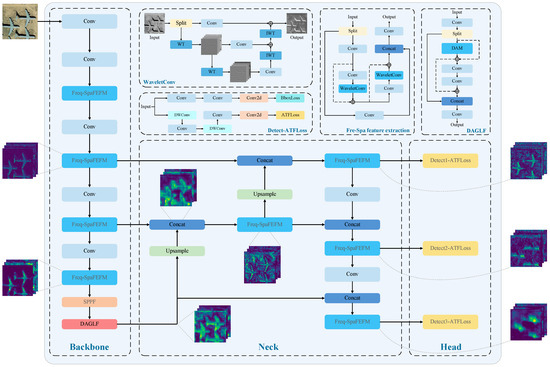
Figure 1. Network architecture of YOLO11-FSDAT (the colored feature map in Figure 1 is a pseudo-color visualization of the feature activation distribution—the colors are only used to show the feature information at different stages and do not represent the real image channel).

3.2. Frequency Domain—Space Feature Extraction Fusion Module

3.2.1. WaveleteConv

Through an analysis of the typical features of remote sensing imagery, we noticed that due to their high resolution and large size, small targets in the image were often arranged in dense spatial patterns and were typically accompanied by a significant amount of complex background noise [25]. This characteristic makes the model prone to missing detections. Figure 2 shows grayscale images from the COCO128 dataset (left) and the DOTAv1 dataset (right), along with their corresponding frequency spectrum images after fast Fourier transform (FFT). It should be noted that the spectrograms in the figure are all grayscale graph visualization results—their grayscale intensity indicates the magnitude size of different frequency components, and the color does not represent the actual color information of the original graph. As observed, the frequency spectrum of the remote sensing images exhibited a distinct “cross-shaped” highlighted region that extends outward, indicating a significant presence of periodic high-frequency components in the image. In contrast, the frequency spectrum of the ordinary image on the left has its highlights concentrated at the center, signifying that the image predominantly contained low-frequency components. This comparative experiment demonstrated that extracting more high-frequency information from remote sensing images can significantly enhance the model’s detection performance in object detection tasks, while the effective utilization of such high-frequency features can substantially improve the network’s robustness in complex scenarios [26].

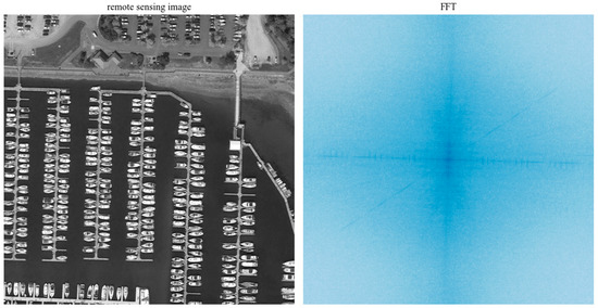
Figure 2. Grayscale images of example images and their frequency spectrum after fast Fourier transform (the spectrogram in the figure is the result of the magnitude visualization of the image after FFT, and the gray intensity indicates the energy distribution of the frequency components).

However, the image obtained after Fourier transform lost spatial information and performing convolution on the frequency spectrum did not hold much significance. Inspired by WTConv [27], we chose wavelet transform, a time–frequency analysis tool, to extract sub-bands of different frequency components from the image while retaining the spatial information. This allowed the convolutional kernels operating on high-frequency sub-bands to more accurately capture the key high-frequency component information in the image. Furthermore, the frequency features contained rich information about scale, texture, and angle, which can be a good complement to the spatial features [28].

Figure 3 shows the sub-band images obtained after performing two-level discrete Haar wavelet transform on the remote sensing image from Figure 2. It should be noted, in particular, that the colors in the plots are used for visualization purposes only. The proximity maps are still in grayscale and represent the low-frequency backbone information, while the detailed component maps are rendered in blue pseudo-colors, which are used to show the high-frequency texture details in different directions more clearly, and are not the original color information of the image.

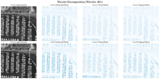
Figure 3. Sub-band images obtained after performing two-level discrete Haar wavelet transform on the remote sensing image (from the DOTAv1 dataset). The blue detail map in the figure shows the results of the visualization of the wavelet high-frequency sub-bands, which are used to enhance the readability of the high-frequency information.

In dense detection tasks for remote sensing images, target edge features often manifest as high-frequency signals, particularly evident in the final three columns. In contrast, the first column on the left contains more complex low-frequency background information, which can interfere with the convolution layer’s ability to extract key features. The high-frequency sub-bands after wavelet decomposition mainly represent the edge information of the target. Performing convolution on these high-frequency sub-bands helps the convolutional kernel capture the crucial edge information of the target, while minimizing the impact of cluttered background information.

As can be observed from the comparison between Figure 2 and Figure 3, the wavelet transform demonstrated significant advantages over the Fourier transform in preserving spatial information. The Fourier transform converted the entire image into the frequency domain, where each frequency component corresponded to the whole image area, resulting in complete loss of positional information and making it difficult to locate the spatial positions of specific frequency components within the image. While this global processing approach is suitable for periodic and stationary signals, it proves inadequate for remote sensing images rich in local details and sharp edges. In contrast, the wavelet transform performed multi-scale analysis using localized window functions at different scales, enabling simultaneous provision of both frequency and spatial information—known as the “time–frequency localization” property. This means wavelets can precisely capture the specific locations of high-frequency texture features in images, making them particularly suitable for processing key visual characteristics, such as edges, textures, and corner points. By decomposing the image into multi-level high- and low-frequency components, wavelets not only preserve the main image structure (low frequency) but also extract directional high-frequency details, significantly enhancing the representation of object boundaries and structural features in remote sensing images. Therefore, in remote sensing object detection tasks, wavelet transforms are more effective than Fourier transforms in maintaining spatial information and improving detail perception, enabling networks to achieve better performance when detecting densely distributed small objects or structurally complex targets.

As illustrated in Figure 4, the WaveleteConv architecture employs a tensor parallel replication mechanism. The input feature map $X$ is duplicated along the batch dimension to generate two identical computational branches, $X_1$ and $X_{\mathbf{2}}$, which subsequently undergo multi-scale wavelet decomposition and cross-branch feature fusion:

$$X_{\mathbf{2}}=X_1$$

(1)

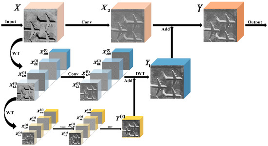
Figure 4. Information flow of WaveletConv (the input grayscale image is from the DOTAv1 dataset, showing how the image flows through WaveletConv and how the feature maps change). The color shades in the figure reflect the response intensity in different regions of the feature map, which is used to visualize the information flow changes in each stage of WaveletConv.

The branch $X_1$ undergoes a wavelet transform (WT) first, which splits it into four sub-bands: “HH,” “HL,” “LH,” and “LL”:

$$X_{LL}^{\left(1\right)},X_{LH}^{\left(1\right)},X_{HL}^{\left(1\right)},X_{HH}^{\left(1\right)}=WT\left(X_1\right)$$

(2)

Then, the $X_{LL}^{\left(1\right)}$ sub-band undergoes another wavelet transform, which is also split into four sub-bands:

$$X_{LL}^{\left(2\right)},X_{LH}^{\left(2\right)},X_{HL}^{\left(2\right)},X_{HH}^{\left(2\right)}=WT\left(X_{LL}^{\left(1\right)}\right)$$

(3)

After the second-level wavelet transform, the four sub-bands, $X_{LL}^{\left(2\right)},X_{LH}^{\left(2\right)},X_{HL}^{\left(2\right)}$, and $X_{HH}^{\left(2\right)}$, each pass through a convolution layer, and then an inverse wavelet transform (IWT) is utilized to recover $Y^{\left(2\right)}$:

$$Y^{\left(2\right)}=IWT\left(Conv\left(X_{LL}^{\left(2\right)}\right),Conv\left(X_{LH}^{\left(2\right)}\right),Conv\left(X_{HL}^{\left(2\right)}\right),Conv\left(X_{HH}^{\left(2\right)}\right)\right)$$

(4)

Afterward, $Y^{\left(2\right)}$ is added to the four sub-bands $X_{LL}^{\left(1\right)}$, $X_{LH}^{\left(1\right)}$, $X_{HL}^{\left(1\right)}$, and $X_{HH}^{\left(1\right)}$ from the first wavelet transform, which have also passed through the convolution layer. The result is then subjected to an inverse wavelet transform (IWT) to obtain $Y_1$:

$$X^{\left(1\right)}=\left\{Conv\left(X_{LL}^{\left(1\right)}\right),Conv\left(X_{LH}^{\left(1\right)}\right),Conv\left(X_{HL}^{\left(1\right)}\right),Conv\left(X_{HH}^{\left(1\right)}\right)\right\}$$

(5)

$$Y_1=IWT\left(X^{\left(1\right)}+Y^{\left(2\right)}\right)$$

(6)

Finally, $Y_1$ is added to $Y_2$, which has passed through a convolution layer, resulting in the final output $Y$ of the wavelet convolution:

$$Y=Y_1+X_2$$

(7)

3.2.2. Freq-SpaFEFM

The proposed frequency–spatial feature extraction fusion module (Freq-SpaFEFM) aims to efficiently address challenges, such as complex background with noise, small and densely arranged targets, and significant size differences between targets. Specifically, the Freq-SpaFEFM module innovatively combines time–frequency domain analysis with spatial-domain feature extraction strategies. Through the collaboration of convolutional branch structures and the WaveletConv module, it significantly improves detection accuracy for both small and large objects in remote sensing imagery.

As illustrated in Figure 5, the input feature map was first processed by a convolutional layer to generate feature map $X_{\mathbf{2}}$, which was then evenly split along the channel dimension into continuous sub-tensor branches, a and b, using a Split operation. One of these branches, a, was fed into a region called the “Fre-Spa feature extraction” area, where frequency-domain and spatial-domain features are jointly extracted. In this region, the feature map was first split into two consecutive sub-branches, a1 and a2, using a Split operation. Each branch contained half of the original number of channels. This design ensured that different branches focus on extracting multi-scale and multi-level fine-grained information. Then, branch a1 will undergo sequential feature extraction through two Conv–WaveletConv combination blocks. Each combination block was designed with residual connections (represented by yellow dashed lines) [29], further enhancing the flexibility and diversity of feature flow within the module. This effectively alleviated feature degradation and gradient vanishing problems that can occur in deep networks.

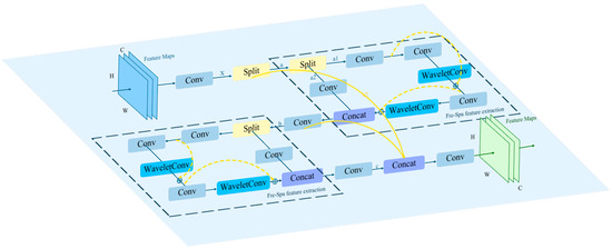
Figure 5. Structural diagram of the Freq-SpaFEFM module.

Afterward, the a2 branch passed through a convolutional layer and was then concatenated with a1 along the channel dimension to fuse the features extracted by each sub-branch. The resulting feature map b was then output from the Fre-Spa feature extraction region. In this region, thanks to the time–frequency domain characteristics of the WaveletConv module, the module can effectively filter out low-frequency background noise that interferes with the features in remote sensing images, while highlighting important information, such as the contours and edges of small targets in the high-frequency sub-bands. Therefore, performing convolution on the high-frequency sub-bands effectively extracted the key features of small targets. At the same time, larger targets, which are usually preserved in the low-frequency sub-bands along with background noise, can still have their features extracted by performing convolution on the low-frequency sub-bands. The background noise primarily interfered with small targets, so convoluting the low-frequency sub-bands helped in extracting the features of large targets as well. Additionally, thanks to the downsampling operation of the wavelet transform (WT) and its time–frequency analysis properties, the receptive field during convolution on the sub-bands was mapped to a larger area of the original image [27]. Specifically, applying a $3\times 3$ convolution to the sub-bands in the second-level wavelet domain of the WaveletConv module will map back to a $12\times 12$ area of the original image through the inverse wavelet transform (IWT). This expansion of the receptive field undoubtedly enhanced the model’s ability to extract features of large-sized targets. Subsequently, the frequency domain features, which have been filtered and enhanced, were reconstructed into the spatial domain through an inverse wavelet transform (IWT). After the feature map b passed through a $1\times 1$ convolution layer to adjust the channel number, it entered another identical second-level Fre-Spa feature extraction region. The output feature map c, after being processed by a Concat operation and a convolution layer, was fused with feature map $X$ and the output feature map b from the first-level Fre-Spa feature extraction region. This fusion formed a rich feature representation that incorporated deep and shallow information, large and small receptive fields, and both frequency domain and spatial information. The ability to detect targets of different scales, particularly closely located small ones, was notably enhanced, and the model became more robust to background interference in remote sensing images.

3.3. Deformable Attention Global Feature and Local Feature Fusion Module (DAGLF)

3.3.1. Deformable Attention Module

In various computer vision tasks, the attention mechanisms are highly regarded for their ability to capture global dependencies. Traditional attention mechanisms mainly include global self-attention (e.g., vision transformer) and local self-attention (e.g., Swin transformer, PVT). Global self-attention computes dependencies across all positions, enabling the capture of long-range dependencies. However, this comes with a significant computational and memory cost and can sometimes lead to attention being distributed to irrelevant information. On the other hand, local attention uses fixed windows or downsampling strategies, which are computationally more efficient but are often data-independent, potentially overlooking crucial global information or long-range relationships. The deformable attention transformer (DAT) addressed these issues by introducing a data-dependent deformable self-attention mechanism. It started by generating a uniform reference point grid on the input features. Then, a lightweight offset network dynamically generated offsets based on the queries, mapping the keys and values to more representative local regions. At the same time, it captured spatial geometric information more precisely through deformable relative position biases, allowing for finer-grained attention to important areas. This design significantly reduced computational complexity and memory overhead while adaptively focusing on important regions. It effectively balanced global contextual dependencies with local feature details, thereby enhancing performance in image classification, object detection, and semantic segmentation tasks [30].

DAM is a key component of the deformable attention transformer (DAT). In the previous section, we proposed methods for addressing missed and misdetected small and densely arranged targets. However, in remote sensing images, there is another scenario where small targets are sparsely distributed in high-resolution images. Traditional multi-head attention mechanisms, for input features $x\in R^{H\times W\times C}$ (where $H$ and $W$ represent image height and width, and $C$ represents the number of channels), typically map the input to query, key, and value spaces through a $1\times 1$ convolution:

$$q=x{W}_q,k=x{W}_k,v=x{W}_{v}C,$$

(8)

where $W_q,W_k,W_v\in R^{C\times C}$ is the linear projection matrix. In multi-head attention, the channel $C$ is divided into $M$ attention heads, with each head having a dimension of $d={\displaystyle \frac{C}{M}}$. For the $m$-th head, its attention output is:

$$z^{\left(m\right)}=soft\max \left({\displaystyle \frac{q^{\left(m\right)}{k}^{\left(m\right)T}}{\sqrt{d}}}\right)v^{\left(m\right)},m=1,\dots ,M$$

(9)

Finally, the outputs of all heads were concatenated and passed through the output projection $W_o$ to obtain the final result:

$$z=Concat\left(z^{\left(1\right)},\dots ,z^{\left(M\right)}\right)W_o$$

(10)

This global dependency modeling performed excellently in capturing the overall semantics of an image, but in remote sensing images, where the target regions are often small and sparsely distributed, directly applying global dense attention introduced a large amount of irrelevant background information, which affected the detection accuracy.

To mitigate this problem, the DAT module incorporated a deformable sampling mechanism. First, the query q was decomposed by groups, dividing the channels C into G groups. The number of channels per group is:

$$C_g={\displaystyle \frac{C}{G}}$$

(11)

The corresponding number of attention heads for each group is:

$$M_g={\displaystyle \frac{M}{G}}$$

(12)

For each group of query features $q_{group}$, a lightweight offset generation network calculated the 2D offset:

$$△p={\theta }_{offset}\left(q_{group}\right),$$

(13)

where ${\theta }_{offset}\left(·\right)$ consists of a depth-wise convolution (grouped convolution) with size $k\times k$, followed by LayerNorm and GELU activation, and then a $1\times 1$ convolution with an output channel size of 2. To prevent the offset from becoming too large, it was normalized using a hyperbolic tangent function and multiplied by an offset range generated from the downsampled size:

$$offset\_range=\left[{\displaystyle \frac{1}{H_K-1}},{\displaystyle \frac{1}{W_K-1}}\right]$$

(14)

Then, multiplying by a predefined scaling factor $offset\_range\_factor$, the normalized offset was obtained:

$$△p^{\prime }=offset\_range\_factor·\tanh \left(△p\right)\odot offset\_range.$$

(15)

Next, we constructed a uniform reference grid $p$:

$$p(i,j)=\left(2{\displaystyle \frac{i+0.5}{H_K}}-1,2{\displaystyle \frac{j+0.5}{W_K}}-1\right),i=0,\dots ,H_K-1,j=0,\dots ,W_K-1.$$

(16)

The offset was added to the reference grid, resulting in the final sampling positions:

$$p\prime =p+△p\prime$$

(17)

The interpolation formula is as follows:

$$\varphi \left(z;\left(p_x,p_y\right)\right)={\displaystyle \sum _{r_x,r_y}\max \left(0,1-\left|p_x-r_x\right|\right)}\max \left(0,1-\left|p_y-r_y\right|\right)z\left[r_y,r_x,:\right]$$

(18)

In remote sensing object detection, this dynamic sampling strategy enables the model to adaptively focus on target regions. Especially in scenarios with significant target size variations and sparse distribution, it effectively enhances the representation of target features.

After dynamic sampling, the DAT module used 1 × 1 convolutions to project the deformed sampled feature elements to generate the keys and values:

$$\tilde{k}=pro{j}_k\left(\tilde{x}\right),\tilde{v}=pro{j}_v\left(\tilde{x}\right)$$

(19)

The original query $q$ was also passed through a $1\times 1$ convolution to retain the full channel information. Then, for each attention head, the shape of the query was rearranged to $\left(B·M,d,H\times W\right)$, while the shapes of the key and value were $\left(B·M,d,N_s\right)$, where the number of sampled points was $N_s=H_K\times W_K$. The multi-head attention calculation formula is:

$$A=soft\max \left({\displaystyle \frac{q{\tilde{k}}^T}{\sqrt{d}}}\right)$$

(20)

It computed the weighted sum to obtain the output of each head:

$$z^{\left(m\right)}=A\tilde{v}$$

(21)

In remote sensing object detection, preserving complete channel information combined with multi-head attention facilitates comprehensive fusion of large-scale structures and small-object features within the image. This makes the model more accurate when handling complex backgrounds.

To further enhance spatial information modeling capabilities, the DAT module introduced relative position encoding in attention calculations. First, the query grid $q_{grid}$ was generated through a function $\_get\_q\_grid$ (normalized coordinates, similar to the reference grid $p$), in the form of:

$$q_{grid}\left(i,j\right)=\left(2{\displaystyle \frac{i}{H}}-1,2{\displaystyle \frac{j}{W}}-1\right),i=0,\dots ,H-1,j=0,\dots ,W-1$$

(22)

The relative displacement between each query position and the sampling position was calculated as:

$$R=q_{grid}-p^{\prime }$$

(23)

The relative displacement $R$ describes the geometric relationship of the target in space and was normalized. Then, using a predefined relative position bias table $\widehat{B}$ (e.g., of shape $\left(2H-1\right)\times \left(2W-1\right)$) and an interpolation function $\varphi \left(\widehat{B};R\right)$, the relative position bias term was calculated as:

$$\varphi \left(\widehat{B};R\right)$$

(24)

Finally, this bias term was added to the attention scores, and the extended attention calculation formula is:

$$Attn=soft\max \left({\displaystyle \frac{q{\tilde{k}}^T}{\sqrt{d}}}+\varphi \left(\widehat{B};R\right)\right)$$

(25)

In remote sensing images, the spatial relationships between targets are often crucial. This mechanism provides the model with precise spatial prior information, which enhances the precision of target localization and detection.

The traditional global attention mechanism typically has a computational complexity of $O\left(H^2{W}^{2}C\right)$ on high-resolution images. However, the DAT module reduced the computational complexity of the offset generation part through dynamic sampling and the grouped shared offset strategy. Let the downsampling factor be $r$, and the number of sampling points be:

$$N_s={\displaystyle \frac{HW}{r^2}}$$

(26)

The overall computational complexity is approximately:

$$\mathrm{\Omega }\left(DMHA\right)=2HW{N}_{s}C+2HW{C}^2+\left(k^2+2\right)N_{s}C$$

(27)

The first term $2HW{N}_{s}C$ corresponds to the dot-product attention computation, the second term $2HW{C}^2$ comes from the full-channel 1 × 1 convolution projection, and the third term $\left(k^2+2\right)N_{s}C$ represents the computational load of the offset generation network. The complexity optimization enabled real-time remote sensing object detection under high-resolution inputs, while maintaining low computational and memory overhead.

In summary, dynamic sampling automatically focused on the target area, multi-head attention and full-channel projection ensured that target details were not lost, and relative position encoding provided more refined spatial prior information. Additionally, the optimization of computational complexity met the real-time detection requirements for large-scale high-resolution images. Therefore, the DAM is well-suited as an efficient and robust attention mechanism module in the field of image object detection.

3.3.2. Deformable Attention Global Feature and Local Feature Fusion Module

Although the DAM offers excellent dynamic attention performance and relatively lightweight computational complexity, it is inherently based on the transformer architecture, which emphasizes global information modeling. Direct insertion of this module may result in local features being diluted by global information, thereby reducing the model’s sensitivity to fine-grained target detection.

We designed the DAGLF module, which retains the convolutional layer in C2PSA for extracting local features and introduces the global information captured by the DAM and the spatial sensitivity due to dynamic sampling, to combine the advantages of the two network architectures and thus achieve higher accuracy and robustness in remote sensing image target detection. Specifically, after the feature map entered the DAGLF module, it first passed through a Conv layer, and then was split into two parts, $x_1$ and $x_2$. The feature map $x_2$ underwent the DAM, first passing through a $1\times 1$ Conv layer with 2C output channels, followed by another $1\times 1$ Conv layer with C output channels, resulting in $y_2$, thus performing an operation similar to a fully connected layer:

$$y_2=f\left(Con{v}_2\left(f\left(Con{v}_1\left(x_2\right)+b_1\right)\right)+b_2\right)$$

(28)

where $Con{v}_1$ and $Con{v}_2$ correspond to convolutional layers for channel expansion and compression, respectively, with $f\left(\cdot \right)$ representing the activation function. This feed-forward network structure effectively applied a fully connected transformation at each spatial location, providing additional nonlinear mapping for pixel-level features without significantly increasing computational overhead, thereby further enhancing the feature representation capability. Additionally, considering the deep network layers of the module, residual connections [29] were designed for both the DAM and the Conv layers to provide smoother gradient flow during backpropagation. This helped mitigate the risk of gradient vanishing as the network depth increased, allowing the network to maintain the flow of gradients on the “original input path” even after introducing the attention module. On the other hand, the attention mechanism combined with the residual connections can be seen as the original features plus supplemental features from the attention mechanism’s output:

$$x_{out}=x_{in}+x_{atten}$$

(29)

Global information from attention mechanisms is progressively used to complement convolutional local features, enabled by the structure during training.

However, the feature map $y_2$ was not directly output. Since this module was embedded into the final layer of the backbone network, we first concatenated $y_2$ and $x_1$ along the channel dimension using the Concat operation. Then, a $1\times 1$ convolutional layer was applied to adjust the number of channels, and the result was used as the final output of the module. This architecture enriched feature representation by combining global semantics from the module with backbone-derived local features, which is vital for managing large inter-class scale variations in remote sensing tasks. Figure 6 visualizes the DAGLF module’s structure.

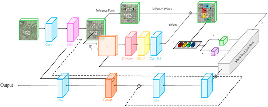
Figure 6. The structural block diagram of the DAGLF module.

3.4. Adaptive Threshold Focal Loss

In remote sensing image object detection, imbalanced sample distribution across categories is a prevalent issue, primarily arising from the inherent class composition of the datasets. Using the traditional loss functions, such as cross-entropy loss, often leads to significantly poorer detection performance for classes with fewer samples compared to others. Although the classic focal loss mitigates the impact of easily classified samples by introducing a modulation factor ${\left(1-p_t\right)}^{\gamma }$, it also reduces the loss weight for difficult samples, which is detrimental to the learning of challenging samples. To address this issue, we adopted the adaptive threshold focal loss (ATFL), which is a dynamic loss function that adjusts sample weights based on classification difficulty. By decoupling easily and difficultly classified targets, it suppresses the influence of easy samples and emphasizes learning from hard examples, thereby enhancing model performance on imbalanced remote sensing datasets. ATFL combines the targeted nature of threshold decoupling and the flexibility of adaptive weight adjustment, enabling adaptive focusing based on sample difficulty [31]. It is capable of addressing more difficult samples while effectively mitigating the imbalance between foreground objects and background regions.

The classic cross-entropy loss function can be represented as:

$$L_{BCE}=-\left(y\log \left(p\right)+\left(1-y\right)\log \left(1-p\right)\right)$$

(30)

where $p$ represents the predicted probability, and $y$ represents the true label, which can be succinctly expressed as:

$$L_{BCE}=-\log \left(p_t\right)$$

(31)

where

$$p_t=\left\{\begin{array}{cc}p,& if y=1\\ 1-p,& others\end{array}\right.$$

(32)

The standard cross-entropy loss is insufficient for handling sample imbalance issues. Therefore, the focal loss function introduced a modulation factor ${\left(1-p_t\right)}^{\gamma }$ and adjusted the focusing parameter $r$ to reduce the loss contribution of easily classified samples. The focal loss function can be expressed as:

$$FL\left(p_t\right)=-{\left(1-p_t\right)}^{\gamma }\log \left(p_t\right)$$

(33)

Although modulation reduces the impact of easy samples, it simultaneously diminishes the gradient contribution of hard examples, which adversely affects their learning. To address this issue, the threshold focal loss (TFL) function was introduced, which reduces the loss weight of easily classified samples while increasing the loss weight assigned to difficult samples, effectively mitigating the impact of easy samples. Specifically, prediction probability values above 0.5 were designated as easy samples, and those above this threshold were considered difficult samples. The TFL loss can be expressed as:

$$TFL=\left\{\begin{array}{cc}-{\left(\lambda -p_t\right)}^{\eta }\log \left(p_t\right)& p_t\le 0.5\\ -{\left(1-p_t\right)}^{\gamma }\log \left(p_t\right)& p_t>0.5\end{array}\right.$$

(34)

where $\eta$, $\gamma$, and $\lambda$ (>1) are hyperparameters. For different models and datasets, these hyperparameters need to be adjusted multiple times to achieve optimal performance. In deep learning, each training process takes a significant amount of time, resulting in high time costs. Therefore, the adaptive improvements were made to $\eta$ and $\gamma$.

For the simple samples, the loss value decreased as $p_t$ increased, further reducing the loss generated by simple samples. At the beginning of training, even the simple samples had relatively low predicted probabilities, similar to the difficult samples, and as training progressed, these probabilities gradually increased. $\gamma$ should gradually approach 0. The predicted probabilities of ground truth targets can serve as a mathematical proxy for modeling training progress, and their evolution can be effectively estimated using exponential smoothing. This adaptive improvement can be expressed as:

$${\widehat{p}}_c=0.05\times {\displaystyle \frac{1}{t-1}}{\displaystyle \sum _{i=0}^{t-1}{\overline{p}}_i+0.95\times p_t}$$

(35)

where ${\widehat{p}}_c$ represents the predicted value for the next epoch, $p_t$ represents the current average predicted probability, and $p_t$ represents the average predicted probability for each epoch. According to Shannon’s information theory, the larger the probability value of an event, the smaller the amount of information it brings; conversely, the greater the information amount. Therefore, the adaptive modulation factor $\gamma$ can be expressed as:

$$\gamma =-\ln \left({\widehat{p}}_c\right)$$

(36)

However, in the later stages of model training, an overly large expected probability would reduce the weight of difficult samples. Therefore, we defined $\eta$ as:

$$\eta =-\ln \left(p_t\right)$$

(37)

By combining $\eta$ and $\gamma$ into the TFL, the final expression for ATFL was obtained as:

$$ATFL=\left\{\begin{array}{cc}-{\left(\lambda -p_t\right)}^{-\ln \left(p_t\right)}\log \left(p_t\right)& p_t\le 0.5\\ -{\left(1-p_t\right)}^{-\ln \left({\widehat{p}}_c\right)}\log \left(p_t\right)& p_t>0.5\end{array}\right.$$

(38)

First, the threshold was set to decouple easily classified targets from hard-to-classify targets. Second, by reinforcing the loss related to difficult-to-classify targets and reducing the loss associated with easy-to-classify samples, we forced the model to allocate more attention to the features of difficult targets, thus alleviating the problem of class imbalance. Finally, an adaptive design was applied to the hyperparameters to reduce the time consumption caused by hyperparameter tuning.

In remote sensing object detection tasks, the class imbalance often leads to the underperformance of models in correctly classifying target classes with fewer samples. The integration of ATFL loss with data augmentation strategies effectively enhanced the model’s attention to challenging targets during training, leading to improved detection accuracy.

4. Results

4.1. Description of the Experimental Environment and Dataset

4.1.1. Experiment Environment Settings

The experimental environment used CUDA 12.1 and the Pytorch 2.1.2 deep learning framework, with the operating system being Ubuntu. The model training was performed on an AMD EPYC 9754 @ 2.3GHz processor and an NVIDIA GeForce RTX 4090 GPU, with 300 epochs. Data augmentation techniques were applied, with Mosaic probability set to 1.0, Mixup probability to 0.2, Copy_paste to 0.2, and fliplr to 0.5. None of the models involved in ablation and comparison experiments used pre-trained weights during training.

4.1.2. Evaluate Metrics

In this study, we evaluated the algorithm’s performance by comparing the differences between the pre-improvement model and the post-improvement model under the same image detection experimental setup. The evaluation system for object detection was based on four key metrics: mean average precision (mAP), precision, recall, and F1 score:

$$\mathrm{Precision}={\displaystyle \frac{TP}{TP+FP}}$$

(39)

$$\mathrm{Recall}={\displaystyle \frac{TP}{TP+FN}}$$

(40)

$$AP={\displaystyle {\int }_0^{1}p\left(r\right)}dr$$

(41)

$$mAP={\displaystyle \frac{{\displaystyle \sum _{q=1}^{Q}AP\left(q\right)}}{Q}}$$

(42)

$$F_1=2·{\displaystyle \frac{\mathrm{Precision}·\mathrm{Recall}}{\mathrm{Precision}+\mathrm{Recall}}}$$

(43)

TP (true positive), FN (false negative), and FP (false positive) denote the number of correctly detected targets, missed targets, and incorrectly detected background samples, respectively. Precision and recall were used to evaluate detection accuracy and completeness. The precision–recall curve was used to derive the AP for each class, and mAP was calculated as the mean of all APs across N categories. The F1 score was computed as the harmonic mean of precision and recall.

4.1.3. Experimental Datasets

To validate the detection performance of the improved YOLOv11n network on remote sensing image object detection, the experiments were conducted on three publicly available datasets: DOTAv1, SIMD, and DIOR. The specific details are as follows:

• The DOTAv1 dataset [32] is a large-scale remote sensing dataset specifically designed for aerial image object detection, released by the Wuhan University team in 2018. It contains 2806 aerial images, covering 15 categories with 188,282 instances.
• The SIMD dataset [33] was proposed by the research team from the National University of Sciences and Technology (NUST) in Pakistan in 2020, primarily for vehicle detection tasks. This dataset contains 5000 high-resolution remote sensing images (size 1024 × 768) and is annotated with 45,096 target instances. It has a high proportion of small to medium-sized targets (both width and height smaller than 0.4).
• The DIOR dataset [34] was introduced in 2020 as a comprehensive benchmark for optical remote sensing image object detection. It includes 23,463 images and 190,288 annotated instances, covering 20 object categories (such as airplanes, bridges, ports, vehicles, etc.).

These datasets include a diverse spectrum of detection targets, ranging from small-scale objects to large-scale infrastructure, thereby offering a comprehensive benchmark for assessing detection accuracy and model robustness. Table 1 presents the instance count for each category across the three datasets.

Table 1. The number of instances for each category in the three datasets.

Datasets	DOTAv1		SIMD		DIOR
	Class	Number	Class	Number	Class	Number
1	small vehicle	60,804	car	20,504	airplane	10,104
2	large vehicle	45,499	truck	2802	airport	1327
3	plane	21,724	van	5732	baseball field	5817
4	storage tank	14,667	long vehicle	1622	basketball court	3225
5	ship	80,761	bus	1991	bridge	3967
6	harbor	17,919	airliner	968	chimney	1681
7	ground track field	1159	propeller aircraft	195	dam	1049
8	soccer ball field	1211	trainer aircraft	631	expressway–service area	2165
9	tennis court	6352	chartered aircraft	640	expressway–toll station	1298
10	swimming pool	4183	fighter aircraft	49	goldfield	1086
11	baseball diamond	1231	others	785	groundbreaking	2318
12	roundabout	1102	stair truck	443	harbor	5509
13	basketball court	1420	pushback truck	209	overpass	3114
14	bridge	4622	helicopter	60	ship	62,400
15	helicopter	1326	boat	8672	stadium	1268
16					storage tank	26,414
17					tennis court	12,266
18					train station	1011
19					vehicle	40,370
20					windmill	5363

4.1.4. Analysis of Experimental Results

To verify the target detection performance of the improved YOLO11-FSDAT network in remote sensing images, this paper compared the proposed improved algorithm with the currently mainstream algorithms in the field of remote sensing image target detection, specifically including YOLOv5n, YOLOv8n, YOLOv10n, YOLOv11n, YOLOv12n, and RT-DETR. The mean average precision (mAP) was adopted as the primary evaluation metric for assessing detection performance in the comparative experiments, and the corresponding results are presented in Table 2. To improve readability and facilitate comparison, we used red, blue, and green to label the first, second, and third rankings of the indicators.

Table 2. Comparison of detection results of different models on the DOTAv1 dataset (%).

Methods	YOLOv5n	YOLOv8n	YOLOv10n	YOLOv11n	YOLOv12n	RT-DETR	Ours
small vehicle	71.56	70.95	74.66	69.64	74.82	71.18	75.08
large vehicle	87.52	86.78	88.02	87.59	88.53	85.05	88.74
plane	92.61	92.30	92.65	92.36	93.20	92.64	93.51
storage tank	76.39	76.24	78.93	77.80	78.44	78.89	78.78
ship	90.57	90.41	91.12	90.91	90.65	89.64	91.49
harbor	84.00	84.54	83.01	82.59	84.86	80.37	84.12
ground track field	54.94	56.73	57.90	57.29	62.01	53.59	69.61
soccer ball field	58.34	58.19	63.85	59.19	59.67	55.76	62.88
tennis court	94.91	94.23	94.34	94.16	94.34	92.41	94.80
swimming pool	62.01	60.30	66.31	64.85	67.77	63.33	69.15
baseball diamond	74.27	72.15	75.45	77.42	77.11	79.08	79.60
roundabout	55.82	57.32	58.80	59.52	59.04	63.99	61.74
basketball court	65.20	65.80	63.70	61.41	63.56	59.75	66.08
bridge	46.24	47.78	49.14	45.61	49.96	49.41	53.39
helicopter	47.53	51.30	59.72	46.34	63.25	48.46	59.30
mAP50	70.79	71.00	73.17	71.11	73.82	70.90	75.22

The mAP50 represents the value when the IOU threshold is set to 0.5. Intersection over union (IoU) is a widely used metric that quantifies the overlap between the predicted bounding box and the corresponding ground truth bounding box. The higher the ratio, the better the detection performance. As shown in Table 2, our model achieved a mAP of 75.22% on the DOTAv1 dataset, outperforming YOLOv5n, YOLOv8n, YOLOv10n, YOLOv11n, YOLOv12n, and RT-DETR by 4.43%, 4.22%, 2.05%, 4.11%, 1.40%, and 4.32%, respectively. There were significant improvements in detecting objects, such as “ground track field,” “bridge,” and “swimming pool.” Specifically, the progress in detecting “ground track field” was attributed to the introduction of the Freq-SpaFEFM module, which helped expand the receptive field, enabling the model to extract key information from larger-sized targets. “Bridge” targets often suffer from background similarity and can be easily drowned in background noise. The Freq-SpaFEFM module’s convolutional features across different frequency sub-bands effectively enhanced high-frequency edge features and, combined with the DAGLF module’s ability to focus on key information from large targets, it significantly improved the model’s performance in detecting “bridge” targets. Additionally, as seen in the previous section, the sample sizes of “ground track field” and “swimming pool” targets were relatively small in the dataset. The adaptive threshold focal loss (ATFL) improved the model’s attention to low-frequency and hard-to-detect targets by adaptively adjusting its focus based on sample difficulty, thereby effectively mitigating the class imbalance problem in object detection.

Figure 7 illustrates the detection performance of the enhanced YOLO11-FSDAT model on the DOTAv1, SIMD, and DIOR datasets. The results demonstrate that the three proposed enhancements significantly improved the model’s performance over the baseline across a range of challenging remote sensing scenarios, leading to higher detection accuracy and a reduced missed detection rate.

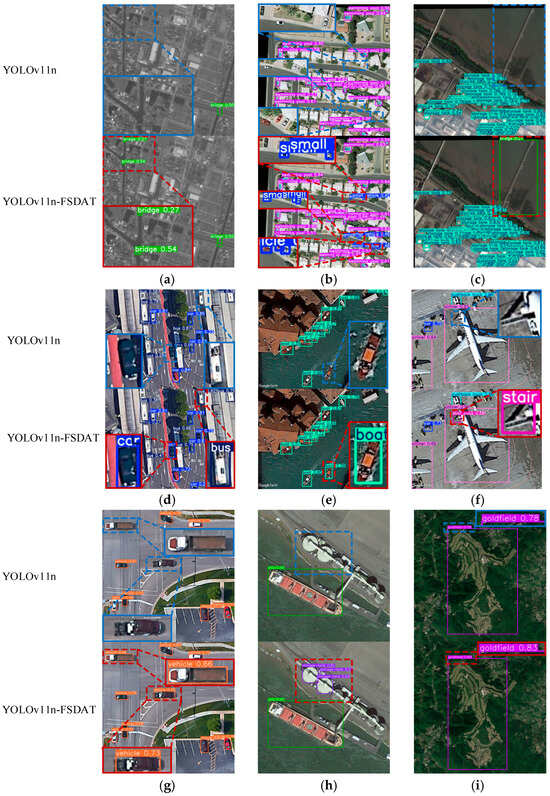
Figure 7. Object detection results of YOLOv11n and YOLO11-FSDAT on remote sensing images. (a) Sample image with complex background noise and small-target scale (DOTAv1 dataset). (b) Densely arranged multi-sample image (DOTAv1 dataset). (c) Multi-sample image with large class size differences (DOTAv1 dataset). (d) Multi-sample image with foreground occlusion (SIMD dataset). (e) Single-class multi-angle small-target sample image (SIMD dataset). (f) Multi-sample image with large class size differences (SIMD dataset). (g) Single-class multi-angle sample image (DIOR dataset). (h) Multi-sample image with large class size differences (DIOR dataset). (i) Single-sample image with high-target-background similarity (DIOR dataset).

Specifically, as shown in Figure 7a, the image had significant background noise, and the target to be detected was small in size, easily drowning in the background noise. Before the improvement, the baseline model only detected one target, but the improved model detected three targets with higher confidence. Additionally, Figure 7d shows a sample with foreground occlusion, where a small car at the lower center is partially blocked by a bus, and a bus in the upper right corner is largely obscured. The baseline model failed to detect these targets, while the improved model detected them both. In Figure 7i, the target to be detected was large in size and very similar to the background. The improved model correctly detected the target, and the confidence level was significantly higher compared to the baseline model.

To further evaluate the detection performance across different target categories, we analyzed the AP, precision, recall, and F1-score for each class in the DOTAv1 dataset based on the proposed improved method, as presented in Table 3. Among all categories, “tennis court” achieved the highest scores across all four metrics, which can be attributed to its moderate object size and relatively clean surrounding background, allowing for more distinctive feature extraction. In contrast, the “bridge” category showed the lowest performance, likely due to its less distinctive structural features and frequent blending with complex backgrounds, resulting in a higher rate of missed detections. In order to improve readability and to facilitate comparison of indicator sizes for different types of detection targets, we used red, blue, and green to label the first, second, and third rankings of indicators. To clearly observe the variations in different metrics across target categories, we plotted bar charts for visualization, as shown in Figure 8.

Table 3. Performance analysis of the improved model for each category in the DOTAv1 dataset.

Class	AP (%)	Precision (%)	Recall (%)	F1 Measure
small vehicle	75.08	75.82	67.25	71.28
large vehicle	88.74	86.21	83.89	85.03
plane	93.51	93.65	87.96	90.72
storage tank	78.78	91.99	62.55	74.47
ship	91.49	91.68	87.43	89.50
harbor	84.12	83.01	81.55	82.27
ground track field	69.61	79.30	58.23	67.15
soccer ball field	62.88	74.21	56.55	64.19
tennis court	94.80	94.99	91.07	92.99
swimming pool	69.15	69.20	74.05	71.54
baseball diamond	79.60	85.31	72.07	78.13
roundabout	61.74	80.34	45.49	58.09
basketball court	66.08	74.40	56.76	64.39
bridge	53.39	71.33	47.43	56.98
helicopter	59.30	51.46	57.46	54.29

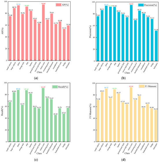
Figure 8. Bar charts of various metrics and categories on the DOTAv1 dataset. (a) Bar chart of objects by category and their AP. (b) Bar chart of objects by category and their precision. (c) Bar chart of objects by category and their recall. (d) Bar chart of objects by category and their F1 measure.

5. Discussion

5.1. Comparative Experiments

To assess the robustness and generalization capability of the proposed model, we performed comparative experiments against several state-of-the-art object detection algorithms, including YOLOv5n, YOLOv8n, YOLOv10n, YOLOv11n, YOLOv12n, and RT-DETR, using three publicly available remote sensing datasets: DOTAv1, SIMD, and DIOR. These datasets differ in terms of scene complexity, object distribution, and scale variation, thus serving as a reliable benchmark for evaluating model performance. The detailed experimental results are presented in Table 4. In order to improve readability and facilitate comparison of the size of the corresponding indicators on different datasets, we used red, blue, and green to label the first, second, and third rankings of the indicators. We plotted bar charts to compare the mAP and precision of each dataset and model, as shown in Figure 9. Additionally, to demonstrate the real-time performance of the model, we plotted a point–line graph showing the relationship between GFLOPs and precision, as shown in Figure 10.

Table 4. Comparative experiments of the three datasets.

Models	DOTAv1			SIMD				DIOR		GFLOPs
	mAP50 (%)	mAP50-95 (%)	Precision (%)	mAP50 (%)	mAP50-95 (%)	Precision (%)	mAP50 (%)	mAP50-95 (%)	Precision (%)
YOLOv5n	70.79	47.61	77.58	79.87	63.41	76.11	84.94	60.81	87.07	5.8
YOLOv8n	71.00	48.12	76.56	80.23	63.53	76.61	86.27	62.71	88.91	6.8
YOLOv10n	73.17	49.80	78.24	79.65	64.52	76.41	86.62	64.54	89.06	8.3
YOLOv11n	71.11	48.71	77.27	78.97	64.24	76.48	87.02	64.52	89.25	6.3
YOLOv12n	73.82	50.47	79.18	80.39	66.09	75.37	87.22	65.25	89.44	6.3
RT-DETR	70.90	46.50	74.98	75.49	61.34	77.54	85.38	62.90	86.21	103.5
Ours	75.22	50.70	80.19	82.79	66.97	77.18	88.01	65.24	90.34	6.3

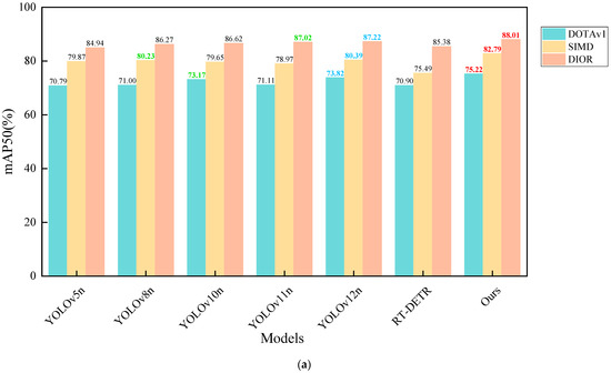
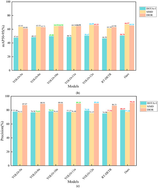
Figure 9. Bar charts of mAP and precision for different datasets and models. (a) Bar charts of mAP50 (%) for different datasets and models. (b) Bar charts of mAP50-95 (%) for different datasets and models. (c) Bar charts of precision (%) for different datasets and models.

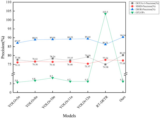
Figure 10. Point–line chart of GFLOPs and accuracy for models on DOTAv1, SIMD, and DIOR datasets.

The results in Table 4 show that YOLO11-FSDAT achieved improvements of 4.11%, 3.82%, and 0.99% in mAP50, and 1.99%, 2.73%, and 0.72% in mAP50-95, compared to its baseline model YOLOv8n on the DOTAv1, SIMD, and DIOR datasets, respectively. This demonstrates the effectiveness of the proposed improvements. Furthermore, our model outperformed YOLOv5n, YOLOv8n, YOLOv10n, YOLO12n, and RT-DETR on all three datasets, showcasing its potential and advantages in remote sensing image object detection tasks. As shown in the Figure 10, our model not only demonstrated excellent accuracy with a high detection rate but also significantly reduced computational load, effectively lowering the demand for computing resources. Overall, the model achieved a good balance between accuracy and efficiency, showcasing strong practical value and potential for widespread application.

5.2. Ablation Experiments

In response to the issues of uneven sample distribution across categories, missed detection in dense small-target scenes, large-scale differences between object categories, and severe background contamination typical of remote sensing object detection scenes, we proposed three network improvement methods in this paper. To evaluate the effectiveness of each method and their optimal combination, we conducted ablation experiments on the DOTAv1 dataset. Method A introduces the frequency–spatial feature extraction fusion module (Freq-SpaFEFM) into the backbone and neck of the network. Method B integrates the dynamic attention global–local fusion module (DAGLF) into the last layer of the backbone. Method C replaces the classification loss with ATFL. The experimental results are presented in Table 5. To improve readability and facilitate comparison of the size of different indicators, we used red, blue, and green to label the first, second, and third rankings of the indicators. At the same time, we plotted bar charts to compare the metrics of different models, as shown in Figure 11. Additionally, to demonstrate the real-time performance of the models, we plotted point–line charts illustrating the relationship between GFLOPs and accuracy, as shown in Figure 12.

Table 5. Results of ablation experiments.

Models	mAP50 (%)	mAP50-95 (%)	Precision (%)	Recall (%)	GFLOPs
YOLOv11n (Baseline)	71.35	48.85	76.64	66.64	6.3
Baseline + A	72.76	49.72	77.35	67.94	6.4
Baseline + B	72.44	49.74	77.99	67.15	6.2
Baseline + C	72.84	48.89	77.83	68.50	6.3
Baseline + A + B	74.20	50.20	79.93	68.65	6.3
Baseline + A + C	73.45	49.27	77.45	70.16	6.4
Baseline + B + C	73.73	49.79	78.26	68.71	6.2
Baseline + A + B + C	75.22	50.70	80.19	68.65	6.3

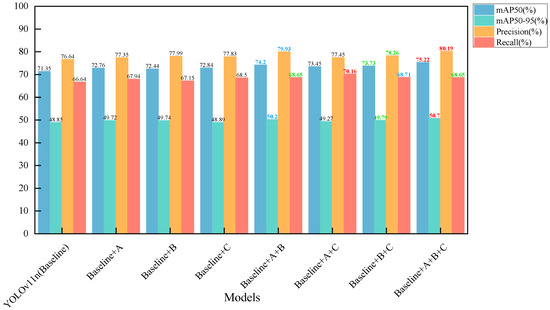
Figure 11. Comparison bar charts of different models’ mAP50 (%), mAP50-95 (%), precision (%), and recall (%).

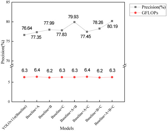
Figure 12. Scatter and line plot of GFLOPs versus accuracy for different models.

The results indicate that each approach significantly contributed to enhancing model performance, and their combination led to optimal outcomes. The training process of the ablation experiment on the DOTAv1 dataset is presented in Figure 13.

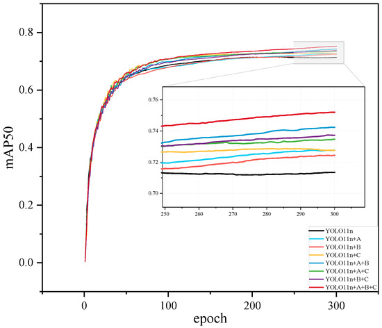
Figure 13. The training process of the ablation experiment on the DOTAv1 dataset.

5.3. Visual Analytics

5.3.1. Visual Analysis of the Freq-SpaFEFM Module

To visually highlight the enhanced feature extraction ability of the Freq-SpaFEFM module, Figure 14 and Figure 15 display the sixth-layer output feature maps for both our model and the baseline model, using a sample image from the DOTAv1 test set. In the baseline, this corresponded to the output of the C3K2 module, while in our model, it corresponded to the Freq-SpaFEFM module.

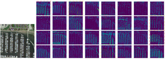
Figure 14. A sample image from the validation set of the DOTAv1 data and the output feature map of layer 6 of our model.

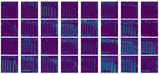
Figure 15. The output feature map of the sixth layer of the baseline model.

First, from an overall perspective, the feature maps output by each channel of the Freq-SpaFEFM module contained more detailed information about the small target “ship.” This was particularly evident in the output feature maps, where more channels highlighted the “ship” at corresponding positions. On a more detailed level, for the small target “ship,” some channels in the feature maps output by the Fre-SpaFEFM module had relatively complete small-target features, with minimal noise (as indicated by the red dashed box in Figure 14). In contrast, the feature maps output by the C3K2 module contained incomplete small-target information and more background noise, as shown by the purple dashed box in Figure 15, where certain small-target positions did not appear highlighted. For the larger target “harbor,” the output feature map from the C3K2 module had only one channel that contained clear and relatively complete target features (as shown by the green dashed box in Figure 15). However, the output feature map from the Freq-SpaFEFM module had three channels that contained clear and relatively complete target features (as shown by the yellow dashed box in Figure 14). This is thanks to the robustness of the Freq-SpaFEFM module in dealing with background noise and its excellent feature extraction capability in dense small-target scenarios, as well as the stronger feature extraction capability for larger targets due to the larger receptive field. These results demonstrate that our Freq-SpaFEFM module had a stronger feature extraction ability in scenarios with dense small targets and large differences in target scales across multiple categories.

5.3.2. Visual Analysis for the DAGLF Module

To more intuitively analyze the superior performance of the DAGLF module, we selected two images from the DOTAv1 test set to extract the attention matrices from the DAGLF module in our model and the C2PSA module in the baseline model, and obtained the attention heatmaps, as shown in Figure 16 and Figure 17, corresponding to small-target images and large-target images. In the figures, (a) represents the original image, (b) represents the attention heatmap output by the DAGLF module, and (c) represents the attention heatmap output by the C2PSA module.

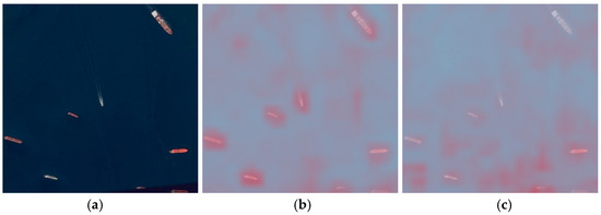
Figure 16. Comparison chart of attention visualization under small-object detection. (a) Validation sample image 1 of DOTAv1 dataset. (b) DAGLF module output image. (c) C2PSA module outputs images.

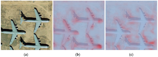
Figure 17. Comparison chart of attention visualization under large-object detection. (a) Validation sample image 2 of DOTAv1 dataset. (b) DAGLF module output image. (c) C2PSA module outputs images.

It is clear that, whether for small targets or larger targets, the DAGLF module exhibited superior performance. When dealing with small targets, the DAGLF module evenly distributed attention to each small target, which is shown as deeper red in the figure, while the C2PSA module failed to assign attention to some targets or assigned lower attention, represented by light blue or light pink in the figure. When dealing with large targets, the DAGLF module accurately allocated attention to key positions of the target, such as the nose and engine in Figure 17b, which are marked with deeper red. The high performance was largely due to the deformable attention’s adaptability and the DAGLF module’s capability for streamlined multi-source information integration.

To further verify the impact of the attention matrix on the final detection results, we selected Figure 18a and used the LayerCAM algorithm to compute the class activation map (CAM) for the tenth layer (where the DAGLF and C2PSA modules are located). As shown in Figure 18, in the class activation map of the DAGLF module, each small target was highlighted, while in the class activation map of the C2PSA module, some small targets were not highlighted. This indicates that with the help of the DAGLF module, the network can indeed focus more effectively on the small targets in the image, reducing the risk of missing small targets and improving the network’s detection performance.

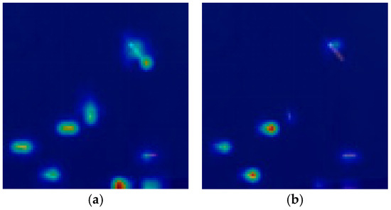
Figure 18. Class activation diagram of layer 10 computed by the LayerCAM algorithm: (a) the class activation map of the DAGLF module and (b) the class activation map of the C2PSA module.

6. Conclusions

This study presented an enhanced architecture based on YOLOv11n, named YOLO11-FSDAT, specifically designed to address the unique challenges of object detection in remote sensing imagery. Built upon the lightweight YOLOv11n framework, the model incorporates three innovative modules: the frequency–spatial feature extraction fusion module (Freq-SpaFEFM), the deformable attention-based global–local feature fusion module (DAGLF), and the adaptive threshold focal loss (ATFL). Together, these components form an efficient detection framework tailored for difficult remote sensing scenarios characterized by small objects, dense object distributions, large-scale variations, and complex backgrounds.

The main findings and contributions of this study are summarized as follows:

• The Freq-SpaFEFM module effectively integrated time–frequency analysis with spatial-domain feature extraction. By adopting a multi-branch architecture that separately processes small and large targets, the module enhanced the model’s ability to detect multi-scale and densely packed objects while suppressing complex background interference.
• The DAGLF module enabled the organic fusion of local details with global contextual information. Through the incorporation of a deformable attention mechanism, the model can adaptively focus on relevant target regions, significantly improving performance on large-scale and fine-grained object detection tasks.
• The ATFL loss function dynamically adjusted loss weights to make the model focus more on hard-to-classify objects. This was especially effective in addressing the long-tailed distribution commonly found in remote sensing data, thereby significantly improving the detection accuracy of underrepresented classes and small-sample targets.
• Experimental results on three public remote sensing datasets—DOTAv1, SIMD, and DIOR—demonstrated that YOLO11-FSDAT outperformed current mainstream methods, including YOLOv5n, YOLOv8n, YOLOv10n, YOLOv11n, and RT-DETR, in terms of detection accuracy. On the DOTAv1 dataset, for instance, the proposed model achieved a mAP50 of 75.22%, representing a 4.11% improvement over the baseline YOLOv11n, validating the model’s superior performance and generalization ability in complex remote sensing scenarios. Additionally, the model exhibited stronger precision and robustness in detecting small, dense, and scale-varying targets within challenging environments.
• The model maintained high detection accuracy while also offering fast inference speed and a lightweight architecture, making it well-suited for real-time deployment and practical applications in diverse remote sensing contexts.

In future work, we plan to incorporate model pruning techniques to eliminate redundant parameters and network connections, achieving a more lightweight design and reducing computational overhead without compromising accuracy. At the same time, we aim to further enhance the overall robustness, precision, and adaptability of YOLO11-FSDAT to ensure its effective deployment across various real-world applications, thereby advancing the development of intelligent remote sensing technologies.

References

- Hou, L.; Li, F. Lightweight Remote Sensing Image Detection Based on Improved EAF-YOLO. J. Shenyang Univ. Technol. 2025, 44, 7–12. [Google Scholar]
- Cai, Q.; Wang, J.; Liang, H. Remote Sensing Image Object Detection Based on Hybrid Attention and Dynamic Sampling. Comput. Syst. Appl. 2025, 34, 171–179. [Google Scholar]
- Cheng, G.; Han, J.; Guo, L.; Qian, X.; Zhou, P.; Yao, X.; Hu, X. Object detection in remote sensing imagery using a discriminatively trained mixture mode. ISPRS J. Photogramm. Remote Sens. 2013, 85, 32–43. [Google Scholar] [CrossRef]
- Qiu, S.; Wen, G.; Fan, Y. Using Layered Object Representation to Detect Partially Visible Airplanes in Remote Sensing Images. In Proceedings of the 2016 International Conference on Progress in Informatics and Computing (PIC), Shanghai, China, 23–25 December 2016; pp. 196–200. [Google Scholar]
- Cheng, G.; Zhou, P.; Han, J. Learning Rotation-Invariant Convolutional Neural Networks for Object Detection in VHR Optical Remote Sensing Images. IEEE Trans. Geosci. Remote Sens. 2016, 54, 7405–7415. [Google Scholar] [CrossRef]
- Ren, S.; He, K.; Girshick, R.; Sun, J. Faster R-CNN: Towards Real-Time Object Detection with Region Proposal Networks. IEEE Trans. Pattern Anal. Mach. Intell. 2017, 39, 1137–1149. [Google Scholar] [CrossRef]
- He, K.; Gkioxari, G.; Dollár, P.; Girshick, R. Mask R-CNN. In Proceedings of the 2017 IEEE International Conference on Computer Vision (ICCV), Venice, Italy, 22–29 October 2017; pp. 2980–2988. [Google Scholar]
- Ma, H.; Liu, Y.; Ren, Y.; Yu, J. Detection of Collapsed Buildings in Post-Earthquake Remote Sensing Images Based on the Improved YOLOv3. Remote Sens. 2020, 12, 44. [Google Scholar] [CrossRef]
- Luo, S.; Yu, J.; Xi, Y.; Liao, X. Aircraft Target Detection in Remote Sensing Images Based on Improved YOLOv5. IEEE Access 2022, 10, 5184–5192. [Google Scholar] [CrossRef]
- Ahmed, M.; El-Sheimy, N.; Leung, H.; Moussa, A. Enhancing Object Detection in Remote Sensing: A Hybrid YOLOv7 and Transformer Approach with Automatic Model Selection. Remote Sens. 2024, 16, 51. [Google Scholar] [CrossRef]
- Zhao, D.; Shao, F.; Liu, Q.; Yang, L.; Zhang, H.; Zhang, Z. A Small Object Detection Method for Drone-Captured Images Based on Improved YOLOv7. Remote Sens. 2024, 16, 1002. [Google Scholar] [CrossRef]
- Zhu, R.; Jin, H.; Han, Y.; He, Q.; Mu, H. Aircraft Target Detection in Remote Sensing Images Based on Improved YOLOv7-Tiny Network. IEEE Access 2025, 13, 48904–48922. [Google Scholar] [CrossRef]
- Yi, H.; Liu, B.; Zhao, B.; Liu, E. Small Object Detection Algorithm Based on Improved YOLOv8 for Remote Sensing. IEEE J. Sel. Top. Appl. Earth Obs. Remote Sens. 2024, 17, 1734–1747. [Google Scholar] [CrossRef]
- Nie, H.; Pang, H.; Ma, M.; Zheng, R. A Lightweight Remote Sensing Small Target Image Detection Algorithm Based on Improved YOLOv8. Sensors 2024, 24, 2952. [Google Scholar] [CrossRef] [PubMed]
- Hwang, D.; Kim, J.-J.; Moon, S.; Wang, S. Image Augmentation Approaches for Building Dimension Estimation in Street View Images Using Object Detection and Instance Segmentation Based on Deep Learning. Appl. Sci. 2025, 15, 2525. [Google Scholar] [CrossRef]
- Zhao, Y.; Lv, W.; Xu, S.; Wei, J.; Wang, G.; Dang, Q.; Liu, Y.; Chen, J. Detrs beat yolos on real-time object detection. In Proceedings of the IEEE/CVF Conference on Computer Vision and Pattern Recognition (CVPR), Seattle, WA, USA, 17–21 June 2024; pp. 16965–16974. [Google Scholar]
- Li, B.; Fang, J.; Zhao, Y. RTDETR-Refa: A real-time detection method for multi-breed classification of cattle. J Real-Time Image Proc 2025, 22, 38. [Google Scholar] [CrossRef]
- Shi, Y.; He, Q.; Mao, C.; Ge, Y.; Du, H.; Wang, H. The Object Detection in Remote Sensing Images Based on Improved YOLO11 with LDConv. In Proceedings of the 2024 6th International Conference on Robotics, Intelligent Control and Artificial Intelligence (RICAI), Nanjing, China, 6–8 December 2024; pp. 605–609. [Google Scholar] [CrossRef]
- Zhao, H.; Jia, L.; Wang, Y.; Yan, F. Autonomous UAV Detection of Ochotona curzoniae Burrows with Enhanced YOLOv11. Drones 2025, 9, 340. [Google Scholar] [CrossRef]
- Agrawal, A.; Papreja, N.; Singh, A.A.; Bhurani, K.; Minocha, S. YoloNet: Hybrid YOLO11 and EfficientNet for Lumpy Skin Disease Detection. In Proceedings of the 2025 3rd International Conference on Device Intelligence, Computing and Communication Technologies (DICCT), Dehradun, India, 21–22 March 2025; pp. 63–67. [Google Scholar] [CrossRef]
- Huang, Z.; Zhao, Y.; Liu, Y. Adaptive YOLOv8-based target detection algorithm for remote sensing images. Commun. Inf. Technol. 2025, 3, 129–133. [Google Scholar]
- Liu, X.; Gong, W.; Shang, L.; Li, X.; Gong, Z. Remote Sensing Image Target Detection and Recognition Based on YOLOv5. Remote Sens. 2023, 15, 4459. [Google Scholar] [CrossRef]
- Wang, X.; Yi, J.; Guo, J.; Song, Y.; Lyu, J.; Xu, J.; Yan, W.; Zhao, J.; Cai, Q.; Min, H. A Review of Image Super-Resolution Approaches Based on Deep Learning and Applications in Remote Sensing. Remote Sens. 2022, 14, 5423. [Google Scholar] [CrossRef]
- Putty, A.; Annappa, B.; Prajwal, R.; Perumal, S.P. Semantic Segmentation of Remotely Sensed Images using Multisource Data: An Experimental Analysis. In Proceedings of the 2024 15th International Conference on Computing Communication and Networking Technologies (ICCCNT), Kamand, India, 24–28 June 2024; pp. 1–6. [Google Scholar] [CrossRef]
- Qu, B.; Li, X.; Tao, D.; Lu, X. Deep semantic understanding of high resolution remote sensing image. In Proceedings of the 2016 International Conference on Computer, Information and Telecommunication Systems (CITS), Kunming, China, 6–8 July 2016; pp. 1–5. [Google Scholar] [CrossRef]
- Sun, H.; Luo, Z.; Ren, D.; Du, B.; Chang, L.; Wan, J. Unsupervised multi-branch network with high-frequency enhancement for image dehazing. Pattern Recognit. 2024, 156, 110763. [Google Scholar] [CrossRef]
- Xia, Z.; Pan, X.; Song, S.; Li, L.E.; Huang, G. Vision Transformer with Deformable Attention. In Proceedings of the 2022 IEEE/CVF Conference on Computer Vision and Pattern Recognition (CVPR), New Orleans, LA, USA, 21–24 June 2022; pp. 4784–4793. [Google Scholar]
- Xu, Y.; Pan, Y.; Wu, Z.; Wei, Z.; Zhan, T. Channel Self-Attention Based Multiscale Spatial-Frequency Domain Network for Oriented Object Detection in Remote Sensing Imagery. IEEE Trans. Geosci. Remote Sens. 2024, 62, 5650015. [Google Scholar] [CrossRef]
- He, K.; Zhang, X.; Ren, S.; Sun, J. Deep Residual Learning for Image Recognition. In Proceedings of the 2016 IEEE Conference on Computer Vision and Pattern Recognition (CVPR), Las Vegas, NV, USA, 27–30 June 2016; pp. 770–777. [Google Scholar]
- Finder, S.E.; Amoyal, R.; Treister, E.; Freifeld, O. Wavelet Convolutions for Large Receptive Fields. In Computer Vision–ECCV 2024. ECCV 2024. Lecture Notes in Computer Science; Leonardis, A., Ricci, E., Roth, S., Russakovsky, O., Sattler, T., Varol, G., Eds.; Springer: Cham, Switzerland, 2025; Volume 15112. [Google Scholar]
- Yang, B.; Zhang, X.; Zhang, J.; Luo, J.; Zhou, M.; Pi, Y. EFLNet: Enhancing Feature Learning Network for Infrared Small Target Detection. IEEE Trans. Geosci. Remote Sens. 2024, 62, 590651. [Google Scholar] [CrossRef]
- Xia, G.S.; Bai, X.; Ding, J.; Zhu, Z.; Belongie, S.; Luo, J.; Datcu, M.; Pelillo, M.; Zhang, L. DOTA: A Large-Scale Dataset for Object Detection in Aerial Images. In Proceedings of the 2018 IEEE/CVF Conference on Computer Vision and Pattern Recognition, Salt Lake City, UT, USA, 18–23 June 2018; pp. 3974–3983. [Google Scholar]
- Haroon, M.; Shahzad, M.; Fraz, M.M. Multisized Object Detection Using Spaceborne Optical Imagery. IEEE J. Sel. Top. Appl. Earth Obs. Remote Sens. 2020, 13, 3032–3046. [Google Scholar] [CrossRef]
- Fatima, S.A.; Kumar, A.; Pratap, A.; Raoof, S.S. Object Recognition and Detection in Remote Sensing Images: A Comparative Study. In Proceedings of the 2020 International Conference on Artificial Intelligence and Signal Processing (AISP), Amaravati, India, 10–12 January 2020; pp. 1–5. [Google Scholar]
Disclaimer/Publisher’s Note: The statements, opinions and data contained in all publications are solely those of the individual author(s) and contributor(s) and not of MDPI and/or the editor(s). MDPI and/or the editor(s) disclaim responsibility for any injury to people or property resulting from any ideas, methods, instructions or products referred to in the content. |
© 2025 by the authors. Licensee MDPI, Basel, Switzerland. This article is an open access article distributed under the terms and conditions of the Creative Commons Attribution (CC BY) license (https://creativecommons.org/licenses/by/4.0/).