Abstract
Current state-of-health (SOH) point prediction methods are highly accurate during early cycles. However, the prediction error increases significantly with increasing numbers of battery charging and discharging cycles, especially in the later stages of degradation. This leads to the intensification of uncertainty regarding SOH, which seriously affects the accuracy and safety of judgments about battery failure. To solve this problem and overcome the limitation of human parameter tuning, this study proposes a method for predicting the SOH interval of lithium batteries based on a stochastic differential equation (SDE) and the chaotic evolutionary optimization (CEO) algorithm to optimize the TSKANMixer network. First, battery charge/discharge curves are analyzed, and health features were extracted to establish a SOH estimation model based on TSKANMixer. Then, the hyperparameters of the TSKANMixer model were optimized using the CEO algorithm to further improve the prediction performance. Finally, the prediction of SOH intervals was implemented using SDE based on the CEO-TSKANMixer model. The results show that the CEO optimization brought the RMSE of SOH prediction for the three cells down to no more than 1%, which was 72.70% lower than that of the baseline model. The PICP of the SDE-based interval prediction model exceeded 90% for all of them, and the NMPIW was no more than 6.47%. This indicates that the model can accurately quantify the SOH uncertainty and effectively support the early warning of the risk of battery failure in the late stages of attenuation. The method can also be used for SOH interval prediction for subsequent battery clusters, reducing the computational complexity of cell-by-cell analysis and improving the overall efficiency of battery management systems.
1. Introduction
Lithium-ion batteries have become the preferred power source for electric vehicles, renewable energy storage systems, and portable electronic devices, due to their high energy density, long cycle life, and low self-discharge rate [1,2,3,4,5,6]. However, lithium-ion batteries are subject to performance degradation during use due to factors such as aging of electrode materials, electrolyte decomposition, and interfacial side reactions, and their SOH gradually declines [7]. SOH is typically defined as the ratio of the current battery capacity to its nominal capacity and serves as a key indicator to quantify the degree of battery aging. Although the SOH point prediction method has high accuracy during early cycles, the prediction error increases significantly as the number of cycles increases, especially in the later stages of decay. This reflects the existence of multiple uncertainties in SOH estimation. These uncertainties primarily originate from three sources: first, measurement errors including noise and drift in current, voltage, and temperature sensors; second, model errors arising from structural biases introduced by simplifications in equivalent circuit models or data-driven models of electrochemical processes; and third, operational conditions and the internal heterogeneity of the battery, including manufacturing variations, cycling conditions, and changes in environmental temperature. A single-point prediction cannot fully reflect the above uncertainties. It may lead to an overly optimistic or pessimistic perception of battery health, thereby affecting the assessment of failure risk and the formulation of charge/discharge strategies. For this reason, interval prediction, as an extension of point prediction, quantifies the uncertainty of SOH estimates by generating prediction results that include confidence intervals, thereby playing a positive role in risk warning, decision optimization, assessment of remaining functional life, and system robustness [8,9]. This method is based on the interval prediction framework of SDE and the CEO optimization process, which has a good modular design and can be easily integrated into existing battery management systems to achieve online processing of real-time data and parallel inferences regarding batch battery clusters.
Currently, methods for estimating the SOH of Li-ion batteries mainly include physical model-based methods and data-driven methods [10,11]. The physical model-based approach describes the electrochemical or equivalent circuit characteristics of a battery by building a mathematical model of it. Equivalent circuit models (ECMs) utilize components such as resistance and capacitance to simulate the dynamic behavior of batteries [12]. In contrast, electrochemical models model batteries based on their internal physicochemical reaction mechanisms [13]. In recent years, research based on physical modeling has made some progress. Plett et al. [14,15] proposed an equivalent circuit model based on extended Kalman filtering for real-time estimation of SOH. Andre et al. [16] developed an electrochemical method based on a single-particle model that considered the electrode aging mechanism. However, physical modeling methods typically require accurate parameter identification, complex modeling processes, and limited adaptability to varying working conditions. Additionally, the computational complexity of physical models is high, making it challenging for them to meet the demands of real-time applications.
Given the limitations of physical models, data-driven approaches have received much attention because they do not require an in-depth understanding of the internal mechanisms of batteries [17,18]. Data-driven approaches learn battery degradation patterns from historical data through machine learning or deep learning algorithms. In recent years, methods such as support vector machines [19], random forests [20], long short-term memory networks (LSTMs) [21], and convolutional neural network (CNNs) [22] have been widely used in SOH estimation. Chemali et al. [23] modeled battery degradation data using LSTM networks and achieved high prediction accuracy; Wu et al. [24] proposed a transformer-based SOH estimation method that enhanced the ability to capture long-term dependencies. Jarraya et al. [25] proposed a SOH estimation method based on KAN-LSTM, which provided valuable ideas for combining KAN feature extraction and sequence modeling; however, it was limited by the sequence computation bottleneck and the efficiency of hyperparameter tuning in the LSTM. Based on this, the current study introduced TSMixer to replace LSTM, enabling the model to effectively integrate multi-scale temporal features through a temporal attention mechanism, thereby enhancing its ability to capture long-term and short-term dependencies while reducing computational complexity and gradient vanishing issues. Additionally, TSMixer supports parallel computing, significantly accelerating training and inference speeds while improving the model’s stability and scalability. However, although data-driven methods excel in generalization ability and prediction accuracy, their predictions are typically only point estimates and lack quantification of uncertainty, making it challenging for them to meet the needs of risk assessment in practical applications. This limitation has prompted research to shift toward interval prediction, which offers greater capability for quantifying uncertainty.
Most existing models only provide point predictions and fail to effectively quantify prediction uncertainty, which affects researchers’ judgment of battery failure as well as the development of charging and discharging strategies for the later stages of battery life [26]. In recent years, stochastic differential equations (SDEs) have shown potential in the field of uncertainty quantification due to their ability to model the uncertainty of dynamic systems through stochastic processes. Huang et al. [27] applied an SDE to financial time series forecasting and successfully generated forecasts with probability distributions. Sumit et al. [28] used an SDE to model the dynamic evolution of biological systems and verified its effectiveness in complex systems. Zhang et al. [29] introduced the SDE method into SOH interval prediction for lithium-ion batteries, proving its advantages in characterizing prediction intervals and confidence levels. However, the application of SDEs in predicting battery state of health intervals is still in the initial exploratory stage, with fewer related studies. There is a strong need to further validate its potential in complex time-series modeling. Moreover, the performance of data-driven models is highly dependent on the choice of hyperparameters, such as the learning rate, the number of layers, and the number of neurons. Traditional manual parameter tuning or grid search methods are inefficient, and it is not easy to find optimal solutions in high-dimensional hyperparameter spaces, which limits performance optimization and the practical deployment of models.
To address the above problems, this study proposes a method for estimating the state of health (SOH) interval of lithium-ion batteries, combining a stochastic differential equation network and the TSKANMixer model. The SDE network addresses the limitations of traditional point prediction by incorporating a stochastic process to generate predictions with quantification of uncertainty. The TSKANMixer model combines the Kolmogorov–Arnold network (KAN) and TSMixer architectures, significantly enhancing the ability to model complex nonlinear dynamics during battery degradation through the nonlinear basis functions of the KAN layer and the temporal attention mechanism of the TSMixer. In addition, a chaotic evolutionary optimization algorithm is employed to optimize the hyperparameters of TSKANMixer, which efficiently explores the hyperparameter space by utilizing chaotic mapping and global search mechanisms to enhance model performance further. The main innovations of this paper are as follows:
- (1)
- Battery degradation dynamics are modelled through the stochastic process of the SDE method and prediction intervals are generated with quantification of uncertainty to make up for the shortcomings of traditional point prediction;
- (2)
- The TSKANMixer model is introduced to enhance the nonlinear dynamic modeling capability. The KAN layer captures the complex nonlinear relationships in the battery degradation process through a learnable nonlinear basis function, which, combined with the temporal attention mechanism and the multilayer perceptron module of the TSMixer, significantly enhances the model’s ability to model long-term dependence and dynamic trends;
- (3)
- Efficient exploration of high-dimensional hyperparameter spaces uses the CEO algorithm for chaotic mapping and initialization of populations, combined with evolutionary strategies to overcoming the inefficiencies and limitations of traditional grid searches or manual parameter tuning.
The rest of this paper is structured as follows. Section 2 describes the dataset used in this study and the feature extraction work; Section 3 describes the basic theory of the methodology used in this paper; Section 4 analyzes the results to validate the effectiveness of the methodology proposed in this study; and Section 5 summarizes the work carried out in this study. The overall framework of the paper is shown in Figure 1.
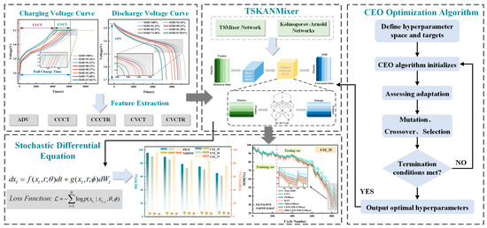
Figure 1.
State-of-health interval prediction framework.
2. Dataset and Preprocessing
2.1. Definition of State of Health
SOH indicates the electrical energy storage capacity of the battery during repeated charging and discharging, which can be defined as the percentage of the maximum usable capacity of the actual battery and its initial rated capacity, as shown in Equation (1) [30,31]:
where denotes the battery’s capacity after cyclic charging and discharging; denotes the initial standard capacity of the battery.
2.2. Introduction to the Dataset
In this study, experiments were conducted using the Center for Advanced Life Cycle Engineering (CALCE) dataset from the University of Maryland [32]. From the CALCE dataset, three sets of battery aging data of lithium-ion batteries numbered CS2_35, CS2_36, and CS2_37 were selected for this experiment. The lithium-ion batteries in the CALCE dataset have all gone through the same charging process, a standard constant current/constant voltage protocol. They were first charged at a constant current at one times their rated capacity until the voltage reached 4.2 V, and then continued to be charged at a constant voltage of 4.2 V until charging stopped when the charging current dropped to 50.0 mA. All were discharged at a constant current of 1.1 A until the voltage of the batteries numbered CS2_35, CS2_36, and CS2_37 dropped to 2.7 V when the discharge was stopped.
2.3. Feature Extraction
Direct measurements cannot be used to determine the SOH of lithium-ion batteries, and indirect estimation is required that involves extracting features that reflect degradation characteristics from the battery’s operating data [33,34]. Taking the CS2_35 battery as an example, this study is based on the characteristics of the battery’s charge/discharge curves, as shown in Figure 2a,b. Five features were extracted from the curves to capture the dynamic behavior of the battery during degradation, as follows:
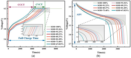
Figure 2.
(a) Charging voltage curve; (b) Discharge voltage curve.
Feature 1: Average discharge voltage (ADV). This feature quantifies the overall voltage level of the battery during the discharge process by calculating the average discharge voltage for each cycle. This feature effectively characterizes the correlation between the cell’s increase in internal impedance and the decrease in SOH, which usually shows a decreasing trend with aging;
Feature 2: Constant current charge time (CCCT). The duration of the constant current charging stage indicates the time required to charge a battery at a constant current. CCCT can reflect the effect of the battery’s internal resistance and capacity changes on the charging process;
Feature 3: Constant current charge time ratio (CCCTR). Defined as the ratio of constant current charging time to total charging time (sum of constant current charging time and voltage charging time). This feature characterizes the relative importance of the constant current phase of the charging process and may show a specific trend as the battery ages;
Feature 4: Constant voltage charge time (CVCT). The duration of the constant voltage charge phase indicates how long a battery will continue to charge after reaching a set voltage. CVCT captures the degradation characteristics of the electrode material and electrolyte during the battery’s aging process.
Feature 5: Constant voltage charge time ratio (CVCTR). Defined as the ratio of constant voltage charge time to total charge time, this feature reflects the proportion of the constant voltage charging phase in the overall charging process, which typically changes as the battery ages, due to increased internal resistance.
The Pearson correlation coefficient (PCC) was used in this study to assess the correlation between the extracted features and SOH [35,36]. The Pearson correlation coefficient was used to measure the linear correlation between the features and SOH, according to the following formula:
where denotes the feature value, denotes the SOH value, and are the mean values of the feature and SOH, respectively, and n is the number of samples. The value of the correlation coefficient r is in the range of [−1,1], with absolute values closer to 1 indicating a stronger correlation. Table 1 shows the correlation between the extracted features and SOH. All five features showed a high correlation (|r| > 0.8), reflecting significant changes with battery capacity decay. The correlation analysis verified their validity for SOH estimation.

Table 1.
Pearson correlation coefficient.
3. SOH Estimation Process and Principle
3.1. Stochastic Differential Equation
Stochastic differential equations are a mathematical tool for modeling dynamic systems by introducing stochastic processes. They can effectively capture a system’s deterministic trends and stochastic fluctuations and are particularly suitable for modeling complex time series with uncertainty [37]. Specifically, in the estimation of lithium-ion battery state of health, a predictive model was first used to perform multi-scale temporal modeling of battery degradation characteristics, outputting a point prediction μ(t). Then, μ(t) was used as input for the drift term f(·) of the SDE model, and a diffusion term g(·) based on training residual statistics was introduced to construct the following equation:
where Xt denotes the stochastic process of battery health status; is standard Brownian motion (Wiener process), introducing randomness, satisfying , i.e., its increment is a random variable that follows a normal distribution with a mean of 0 and a variance of ; is the residual standard deviation of the prediction model on the validation set. By numerically solving this SDE, SOH sample paths that evolve can be generated, and confidence intervals can be constructed at each time point to dynamically quantify the uncertainty of battery health status as it evolves with degradation.
This study used a neural network to parameterize and to construct the SDE network. Specifically, the SDE network contained two sub-networks: the drift and diffusion networks. The drift network modeled deterministic changes in SOH through a multilayer perceptron (MLP) with inputs of the current state and time t and outputs of the drift term; the diffusion network, also using the MLP structure, output the diffusion term to quantify the uncertainty of random fluctuations. Training of the SDE network aimed to reduce the error between the predicted SOH and the actual SOH while enhancing coverage of the prediction interval. To achieve this, Maximum likelihood estimation (MLE) was employed as a loss function, expressed in the following form:
where is the conditional probability density defined by the SDE and N is the number of time steps. During the training process, the SDE was discretized using the Euler–Marshall method to generate a sequence of probability distributions for SOH, which enabled estimation of intervals.
3.2. TSKANMixer Model
The TSKANMixer model is a neural network architecture designed for time-sequence prediction. It is particularly suitable for dealing with the complex nonlinear dynamics and long-term dependencies in SOH prediction for lithium-ion batteries by fusing the time-series processing capability of TSMixer with the nonlinear modeling capability of the Kolmogorov–Arnold network [38]. SOH prediction requires modeling the nonlinear variations and long-term trends of multidimensional features during battery degradation while coping with dynamic perturbations caused by operating conditions. The TSKANMixer significantly improves the model’s accuracy in modeling SOH time series by combining the temporal attention mechanism of the TSMixer with the nonlinear basis functions of KAN.
3.2.1. TSMixer Principle
TSMixer is a hybrid architecture designed for time series forecasting that combines a multilayer perceptron (MLP) and an attentional mechanism [39,40] designed to capture long-term dependencies and interactions between features in time series [41]. For SOH prediction, the TSMixer models the dynamic evolution of SOH over time and operating conditions using a multidimensional sequence of features as input. Its core components include the following.
A temporal attention layer captures the dependencies between different time steps in the time series through the self-attention mechanism. The decaying trend of SOH may be related to charging and discharging behavior hundreds of cycles ago, and the temporal attention layer highlights the contributions of key time steps by calculating the attention weights. Its calculation formula is as follows:
where Q, K, and V are the query, key, and value matrices, respectively, and dk is the dimension of the key. The temporal attention layer maps the input sequence (T is the time series length, and F is the feature dimension) to a weighted feature representation, emphasizing historical information related to SOH changes.
The feature blending layer is a fusion of multidimensional features within the MLP to capture the interaction effects between features. The feature blending layer performs a nonlinear transformation of the feature vector at each time step, expressed as follows:
where W1, W2, b1, b2 are parameters of the MLP.
To avoid gradient vanishing, TSMixer introduces residual connectivity after the temporal attention and feature mixing layers in the following form:
For multi-layer stacking, the TSMixer progressively extracts higher-order features of the SOH time series by stacking multiple layers of temporal attention and feature mixing to ensure that the model can capture long-term degradation trends as well as short-term fluctuations. The specific structure of the TSMixer is shown in Figure 3. The TSMixer enhances the ability to model the long-term dependence of SOH through a temporal attention mechanism, captures the dynamic interactions between features through a feature mixing layer, and is suitable for dealing with complex time-series properties in battery degradation data. However, the TSMixer’s ability to model nonlinear relationships is limited by the expressive power of the MLP, and thus, to further improve performance, a KAN layer needs to be introduced.
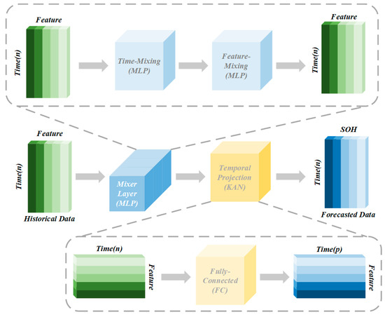
Figure 3.
TSMixer structure.
3.2.2. Kolmogorov–Arnold Network Principle
A Kolmogorov–Arnold network is based on the Kolmogorov-Arnold representation theorem, which approximates complex functions through learnable nonlinear basis functions and has greater expressive power than traditional multilayer perceptrons [42]. For SOH prediction, the KAN models the nonlinear relationship between features. The mathematical expression of the KAN is as follows:
where is the input feature vector, is the learnable univariate basis function, is the outer activation function, and N is the output dimension. The computational process of the KAN is divided into two steps.
For inner basis function processing, each input feature xj is nonlinearly transformed by a set of basis functions to generate an intermediate representation . The basis functions usually take the form of B-spline functions:
where is the B-spline basis function, is the learnable coefficient, and K is the number of basis functions.
The intermediate representation is further mapped by the outer layer activation function to generate the final output. The outer layer activation function enhances the KAN’s ability to fit complex nonlinear relationships.
Compared with traditional MLPs, KAN reduces the number of layers required through learnable basis functions while improving the efficiency of modeling high-dimensional nonlinear relationships. For SOH prediction, the KAN layer can capture complex interactions between features, thus providing richer feature representations for they TSMixer.
3.2.3. TSKANMixer Overall Architecture
The TSKANMixer provides an efficient SOH prediction model by integrating the strengths of a TSMixer and a KAN. It can handle both long-term dependencies of time series and nonlinear relationships among features. Its overall architecture is shown in Figure 4.
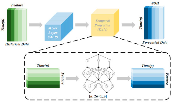
Figure 4.
TSKANMixer structure.
- Time-series input layer
The input layer receives multidimensional time series features shaped like , where T is the time-series length and F is the feature dimension. The input sequences are normalized by Z-score to ensure a consistent magnitude and are divided into multiple time windows to capture degradation patterns at different time scales.
- Parallel processing path
TSKANMixer uses two parallel paths to process the input sequence, as follows:
Along the TSMixer path, the input sequences are processed through the TSMixer module, containing multiple layers of temporal attention and feature mixing. The TSMixer path focuses on modeling the long-term dependencies of the SOH, generating time series feature representations .
Along the KAN path, the input sequences are simultaneously processed through a KAN layer to capture the nonlinear relationships between features. The KAN layer maps the feature vector at each time step to a nonlinear feature representation , ultimately resulting in .
- Fusion layer
The fusion layer integrates the outputs of the TSMixer and KAN paths to generate a comprehensive feature representation. The TSMixer output and the KAN output are merged into through a splicing operation, which is subsequently mapped to the SOH predicted values through a fully connected layer, as follows:
where W and b are the weights and biases of the fully connected layer, and is the SOH prediction at time step t. The fusion layer ensures that the model is capable of both time-series processing and nonlinear modeling by weighting the combination of features from TSMixer and KAN.
- Loss function
The training objective of the TSKANMixer is to minimize the error between the predicted SOH and the true SOH, using the root mean square error (RMSE) as the loss function, as follows:
To prevent overfitting, the L2 regularization term is introduced:
where is the regularization coefficient, and is the model parameter.
For SOH prediction, the TSKANMixer captures long-term decaying trends and short-term fluctuations in SOH through TSMixer paths, models nonlinear interactions between features through KAN paths, and integrates both strengths through a fusion layer. Compared with traditional neural networks, the TSKANMixer has the following advantages: (1) the efficient nonlinear modeling capability of the KAN layer reduces model complexity; (2) the temporal attention mechanism of the TSMixer enhances the capture of long-term dependencies; and (3) the parallel processing and fusion mechanism ensures the full utilization of both feature and temporal information. The output of the TSKANMixer is a point prediction of SOH, which, when combined with the SDE network, further generates interval predictions with quantized uncertainty, providing a highly accurate and reliable basis for decision-making in battery management systems.
3.3. CEO Algorithm Optimization TSKANMixer
The Chaotic evolution pptimization (CEO) algorithm is a population-based meta-heuristic optimization method inspired by a two-dimensional discrete amnesic hyperchaotic mapping, which exploits its hyperchaotic properties to generate stochastic search directions and optimize a high-dimensional parameter space [43]. The CEO framework is similar to the differential evolution algorithm, which contains mutation, crossover, and selection operations, with the core innovation being that the mutation operation employs amnesic hyperchaotic mapping to generate evolutionary directions. In this study, the CEO was used to optimize the learning rate, the number of KAN layer basis functions, the number of TSMixer layers, the number of neurons, the number of iterations, and the batch size parameter of the TSKANMixer model in order to improve the SOH prediction accuracy. The core mechanism of the CEO algorithm is as follows:
- Mutation operation
The variation operation generates evolutionary directions by amnesic hyperchaotic mapping, explores the hyperparameter space, and enhances the global search capability. For optimization of the TSKANMixer, mutation introduces diverse candidate solutions for parameters such as learning rate. The following equation generates individual mutations:
where is the current individual, is the mutated individual, is the random scaling factor, and is the evolutionary direction generated by amnesia mapping. The evolution direction is based on the chaotic candidate individuals generated by the amnesia mapping, which are converted to the parameter space after mapping to the intervals ([−0.5,0.5]) and ([−0.25,0.25]). To accelerate convergence, the optimal solution can be introduced to guide the variation and optimize the local search.
- Crossover operation
The crossover operation combines variant and current individuals through binomial crossover to generate trial vectors that balance exploration and utilization capabilities. For SOH prediction, crossover ensures that the hyperparameter combination retains good properties while introducing new variations. The crossover formula is as follows:
where denotes the jth dimension of the trial vector ui, denotes the jth dimension of the variant individual vi, denotes the jth dimension of the current individual xi, is a randomly selected dimension ensuring that at least one of the dimensions comes from the variant individual. Dim is the dimension of the optimization problem; is the jth dimension of the generated random number, and is the random cross control parameter.
- Selection operation
The selection operation uses a greedy criterion that compares the fitness of the test vector and the current individual and selects the better one for the next generation to ensure that the population converges to the optimal hyperparameter combination. The selection formula is as follows:
where denotes the fitness function. As shown in Figure 5, the process of optimizing the TSKANMixer model via the CEO algorithm can be briefly described as follows:
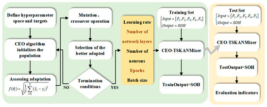
Figure 5.
CEO algorithm optimization process for TSKANMixer.
Step 1: Determine the hyperparameter space and objective function to be optimized, and select hyperparameters, such as the learning rate, number of KAN layer basis functions, number of TSMixer layers, number of neurons, number of iterations, and batch size, to minimize the root mean square error (RMSE) on the validation set;
Step 2: Initialize the population, using logistic mapping to generate the initial population (size 50). Each individual corresponds to a set of hyperparameter configurations and is mapped according to a predetermined range to ensure comprehensive coverage of the search space;
Step 3: Evaluate fitness by training the TSKANMixer model for each individual (hyperparameter combination) and calculating its RMSE on the validation set as the fitness value, to serve as the basis for evaluation in subsequent evolution;
Step 4: For the mutation operation, introduce memristive super chaotic mapping to generate chaotic candidate vectors, combine the current optimal solution and scaling factor, and produce mutated individuals. This step enhances global search capabilities and helps the algorithm escape local optima;
Step 5: For the cross-operation, perform a two-way cross between the mutated individual and itself to generate test vectors, balancing exploration and exploitation by retaining superior genes and introducing random variations;
Step 6: Select an operation, apply the greedy rule, compare the fitness of the test vector and the current individual, and retain the one with the lower RMSE to enter the next generation. Ensure that the algorithm steadily approaches the optimal solution;
Step 7: With regard to iteration and termination, check the termination conditions. If they are not met, execute Steps 2–7, reinitialize the population, and continue the cycle;
Step 8: Apply the optimal hyperparameters. Configure the TSKANMixer model based on the optimal hyperparameter configuration output in Step 7 and verify its improved performance on the test set.
This study selected the CEO algorithm to replace traditional grid search, particle swarm optimization, or genetic algorithms, mainly based on the following considerations:
- Initial population diversity: The CEO algorithm employs chaotic mappings to generate pseudo-random sequences for initializing the population. Compared with purely random or fixed-range initialization methods, this method yields a more uniform distribution of individuals and enhanced employability, thereby improving global search capabilities;
- Escaping local optima: The non-periodic and sensitive dependency characteristics of chaotic sequences can overcome the limitations of traditional evolutionary algorithms, which are prone to falling into local optima, thereby facilitating the algorithm’s escape from traps during iteration and further reducing prediction errors;
- Fast convergence: The CEO algorithm introduces chaotic perturbations into evolutionary operators (selection, crossover, mutation), which can accelerate convergence while ensuring sufficient exploration capabilities, significantly reducing hyperparameter tuning time;
- Parameter adaptation: By dynamically adjusting the mutation rate and crossover rate through chaotic mapping, the CEO algorithm can adaptively balance exploration and exploitation based on the current search state, avoiding premature convergence or excessive randomness.
4. Analysis of Results and Discussion
In order to validate the effectiveness of the SDE-CEO-TSKANMixer model proposed in this study deals with the stochastic degradation noise of the battery SOH by combining stochastic differential equations and optimizes the hyper-parameters of the TSKANMixer by using the chaotic evolutionary optimization algorithm to improve the prediction accuracy and the interval coverage capability of the model. Furthermore, this study included an experimental setup design featuring a 30% training set and a 70% testing set to train and test the SDE-CEO-TSKANMixer. Ablation experiments were conducted to compare and contrast the SDE-TSKANMixer, CEO-TSKANMixer, TSKANMixer, SDE-KAN, SDE-TSMixer, and SDE -CNN models to analyze the role of the SDE and CEO modules in improving prediction performance with regard to SOH intervals. All experiments were performed on a Tensorflow 2.6.0 platform, which was equipped with an NVIDIA Geforce GTX 1650 and 16 GB of RAM.
4.1. Evaluation Metrics
In order to objectively assess the prediction effectiveness of the selected SOH features and the performance of different machine learning models, this study used root mean square error (RMSE), mean absolute error (MAE), mean relative error (MRE), probability of coverage of prediction intervals (PICP), and the normalized mean prediction interval width (NMPIW) as the assessment metrics to evaluate the effectiveness of the models [44]. The formula for these assessment metrics was as follows:
where and are the actual and predicted values of the tth sample, respectively; n is the number of samples; Ut and Lt are the upper and lower bounds of the prediction intervals; I is the indicator function (1 if is within the interval, 0 otherwise); and R is the range of the actual value of SOH. These metrics comprehensively assessed the model’s performance in terms of both the accuracy of point prediction and the reliability of interval prediction.
4.2. SOH Prediction Results
The five extracted features, as stated in Section 2.2, were first used to train the TSKANMixer model. Then, the CEO’s chaotic optimization was further utilized to enhance the global search capability of the hyperparameters, thereby improving the model’s ability to adapt to the complex SOH degradation pattern. The SDE was introduced to achieve SOH interval prediction based on the trained CEO-TSKANMixer model, whose prediction results for the three cells are shown in Figure 6a,c,e. These figures demonstrate the effects of different methods for predicting the SOH of the three cells, respectively. It was observed that different models exhibited significant differences in their performance in predicting the batteries’ state of health. At first, the CNN, TSMixer, KAN, and TSKANMixer models were relatively accurate in their predictions during the early stages of battery cycling. However, as the number of cycles increased, especially when the battery entered the later stages of degradation, the prediction error gradually increased. Among them, the TSMixer performed better than the CNN because the TSMixer included a time-series mixer structure that was better able to capture long-term dependencies in SOH degradation. The KAN model further improved the prediction accuracy through the nonlinear modeling capabilities of the Kolmogorov–Arnold network, exhibiting more minor deviations than the TSMixer in the later stages of decay. The TSKANMixer model combines the time series modeling capabilities of TSMixer with the nonlinear fitting advantages of KAN. It further optimizes feature extraction capabilities through multi-layer attention mechanisms and residual connections, and it yielded the best prediction performance among the aforementioned models. On this basis, the CEO-TSKANMixer model optimized by the CEO algorithm demonstrated superior predictive performance. As shown in the figure, the prediction curve of the CEO-TSKANMixer had the best fit with the actual values, demonstrating the model’s excellent adaptability and stability in long-term predictions.
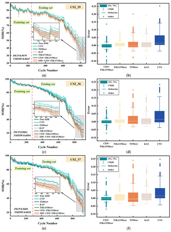
Figure 6.
(a) CS2_35 SOH estimation results; (b) CS2_35 estimation error; (c) CS2_36 SOH estimation results; (d) CS2_36 estimation error; (e) CS2_37 SOH estimation results; (f) CS2_37 estimation error.
From the perspective of error distribution, Figure 6b,d,f include box plots showing the error ranges of the different models. The error distribution of the CNN model was relatively broad and highly volatile. In contrast, the error distributions of the TSMixer and KAN models were more concentrated, with lower overall errors. The TSKANMixer combined the advantages of a TSMixer and a KAN, further converging the error distribution and demonstrating good stability, especially around the median, and further validating the superiority of the TSKANMixer model in terms of predictive performance. Compared with other models, the CEO-TSKANMixer model exhibited lower average error and median values, enabling it to capture changes in battery health more accurately over long-term use.
The specific error data are shown in Table 2. The root mean squared error (RMSE) of the prediction results for the three batteries using the CEO-TSKANMixer model proposed in this study was less than 1%. Taking the CS2_35 battery as an example, the RMSE of the CNN model prediction result waqs 0.0377, while the RMSEs of the TSMixer and KAN models were 0.0290 and 0.0266, respectively, significantly lower than that of the CNN model. Combining the advantages of a TSMixer and a KAN, the prediction error of the TSKANMixer model was further reduced, indicating the correctness of selecting the TSKANMixer model for SOH prediction in this study. The CEO algorithm was used to optimize the parameters of the TSKANMixer model further. The final RMSE of the model’s prediction results was 0.0075, representing a 47.18% reduction in error compared with the baseline TSKANMixer model.
Table 2.
SOH estimation error.
4.3. Comparison of Prediction Results Between Different Model Intervals
As can be seen from Figure 6a,c,e, the prediction error of each method increased gradually as the number of battery charge–discharge cycles increased, leading to increasingly uncertain predictions. Therefore, SDE was introduced to generate prediction intervals with quantified uncertainty. As can be seen from the figure, the SDE-CEO-TSKANMixer network output a narrow prediction interval width for the training dataset, indicating superior training performance and reduced uncertainty in recognizing the training data. However, with the test dataset, the model exhibited more uncertain recognition due to increased battery aging in the later stages of testing. In addition, with comparable accuracy, the SDE-CEO-TSKANMixer network provided uncertainty estimates for the predicted SOH values.
Figure 7 illustrates the PICP and NMPIW values of various models for predicting three battery SOH intervals, allowing further evaluation of the interval prediction performance. The ranges of PICP and NMPIW in the figure are between 0 and 1. For the same PICP, a smaller NMPIW indicates higher interval prediction quality, indicating that the model provides narrower and more accurate prediction intervals [45,46]. Conversely, for the same NMPIW, a larger PICP indicates a greater probability of capturing the actual target value, indicating that the model provided a more reliable and accurate prediction interval. As shown in the figure, the SDE-CEO-TSKANMixer model exhibited the best performance in terms of interval prediction and accuracy. The SDE-KAN and SDE-TSMixer models exhibited similar interval prediction performance, both outperforming the SDE-CNN model. The SDE-TSKANMixer further improved the coverage of the prediction interval. As shown in Table 3, the PICP of the SDE-CEO-TSKANMixer model exceeded 90% in all datasets, and the NMPIW of each dataset did not exceed 6.47%, providing accurate SOH prediction values and reasonable interval estimates. These results indicate that the prediction intervals generated by the SDE-CEO-TSKANMixer model covered most of the data points with relatively narrow interval widths, reflecting the effectiveness and reliability of the SDE-CEO-TSKANMixer network.
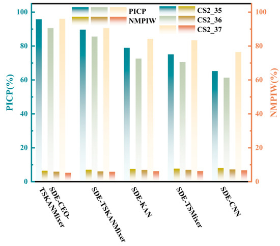
Figure 7.
Comparison of interval prediction performance among different models.
Table 3.
Interval Prediction Evaluation Indicators.
Therefore, the prediction results from all datasets indicated that the SDE-CEO-TSKANMixer model effectively captured the degradation trend of battery SOH and provided reliable prediction intervals. This confirms that the SDE-CEO-TSKANMixer model developed in this study can effectively capture the underlying patterns and relationships in battery datasets with various aging trends, demonstrating the network’s generalization ability and scalability.
5. Conclusions
SOH interval prediction is crucial for lithium-ion battery health management, as it can effectively quantify uncertainties during the degradation process and provide a reliable basis for assessing battery failure and issuing fault warnings. In this study, effective extraction of aging features was performed using multiple cell datasets with fast-charging protocols. A lithium battery SOH interval prediction model based on random differential equations and CEO algorithm optimization of the TSKANMixer model is proposed. The main work and conclusions of this study are as follows:
- (1)
- This study establishes the TSKANMixer model, which combines multi-layer attention mechanisms and residual connections to optimize time series modeling capabilities, providing a foundational framework for lithium-ion battery state-of-health (SOH) prediction and significantly enhancing feature expression capabilities;
- (2)
- The CEO algorithm was used to perform chaotic optimization on the TSKANMixer model, simplifying the manual parameter tuning process. Experimental results demonstrate that the CEO algorithm can improve the global search efficiency of hyperparameters, resulting in a 47.18% reduction in prediction errors compared with the baseline model;
- (3)
- By combining the TSKANMixer network with the SDE network, an SOH interval prediction model was established. Through SDE modeling of degradation uncertainty, the final prediction interval coverage exceeded 90%, and the normalized average prediction interval width did not exceed 6.47%, providing accurate SOH prediction values and reasonable interval estimates.
This study provides a reference for predicting the state of health range of LIBS under conditions of fast charging and can be used for further research on battery cluster range prediction. Future work will focus on three key areas, first, incorporating environmental factors such as temperature and humidity into the model to enhance prediction accuracy; second, designing an online adaptive adjustment mechanism to enable the model to respond to battery aging and changes in operating conditions dynamically; and third, expanding the dataset to include various battery types and charging/discharging protocols, while optimizing processes for handling noise, outliers, and missing values.
Author Contributions
Conceptualization, F.G. and H.H.; methodology, H.H.; software, G.H.; validation, Z.C. and G.H.; formal analysis, F.G.; investigation, G.H.; resources, F.G.; data curation, H.H.; writing—original draft preparation, H.H. and Z.C.; writing—review and editing, F.G.; visualization, G.H.; supervision, H.H.; project administration, F.G. All authors have read and agreed to the published version of the manuscript.
Funding
This research received no external funding.
Data Availability Statement
The data presented in this study are openly available in [Center for Advanced Life Cycle Engineering] at [10.1016/J.EST.2023.107965], reference number [27].
Conflicts of Interest
The authors declare no conflicts of interest.
Abbreviations
The following abbreviations are used in this manuscript:
| SOH | State of health |
| SDE | Stochastic differential equation |
| CEO | Chaotic evolutionary optimization |
| ECM | Equivalent circuit model |
| LSTM | Long short-term memory network |
| CNN | Convolutional neural network |
| KAN | Kolmogorov–Arnold network |
| CALCE | Center for Advanced Life Cycle Engineering |
| ADV | Average discharge voltage |
| CCCT | Constant current charge time |
| CCCTR | Constant current charge time ratio |
| CVCT | Constant voltage charge time |
| CVCTR | Constant voltage charge time ratio |
| PCC | Pearson correlation coefficient |
| MLP | Multilayer perceptron |
| MLE | Maximum likelihood estimation |
| RMSE | Root mean square error |
| MAE | Mean absolute error |
| MRE | Mean relative error |
| PICP | Probability of coverage of prediction intervals |
| NMPIW | Normalized mean pediction interval width |
References
- Shahed, M.T.; Harun-ur Rashid, A.B.M. Battery charging technologies and standards for electric vehicles: A state-of-the-art review, challenges, and future research prospects. Energy Rep. 2024, 11, 5978–5998. [Google Scholar] [CrossRef]
- Jia, C.; Liu, W.; He, H.; Chau, K.T. Deep reinforcement learning-based energy management strategy for fuel cell buses integrating future road information and cabin comfort control. Energy Convers. Manag. 2024, 321, 119032. [Google Scholar] [CrossRef]
- Jia, C.; Liu, W.; He, H.; Chau, K.T. Superior energy management for fuel cell vehicles guided by improved DDPG algorithm: Integrating driving intention speed prediction and health-aware control. Appl. Energy 2025, 394, 126195. [Google Scholar] [CrossRef]
- Li, K.; Zhou, J.; Jia, C.; Yi, F.; Zhang, C. Energy sources durability energy management for fuel cell hybrid electric bus based on deep reinforcement learning considering future terrain information. Int. J. Hydrogen Energy 2024, 52 Pt D, 821–833. [Google Scholar] [CrossRef]
- Ge, M.-F.; Liu, Y.; Jiang, X.; Liu, J. A review on state of health estimations and remaining useful life prognostics of lithium-ion batteries. Measurement 2021, 174, 109057. [Google Scholar] [CrossRef]
- Guo, F.; Huang, G.; Zhang, W.; Wen, A.; Li, T.; He, H.; Huang, H.; Zhu, S. Lithium Battery State-of-Health Estimation Based on Sample Data Generation and Temporal Convolutional Neural Network. Energies 2023, 16, 8010. [Google Scholar] [CrossRef]
- Zhang, J.; Lee, J. A review on prognostics and health monitoring of Li-ion battery. J. Power Sources 2011, 196, 6007–6014. [Google Scholar] [CrossRef]
- Xing, C.; Liu, H.; Zhang, Z.; Wang, J.; Wang, J. Enhancing Lithium-Ion Battery Health Predictions by Hybrid-Grained Graph Modeling. Sensors 2024, 24, 4185. [Google Scholar] [CrossRef]
- Gu, X.; See, K.W.; Li, P.; Shan, K.; Wang, Y.; Zhao, L.; Lim, K.C.; Zhang, N. A novel state-of-health estimation for the lithium-ion battery using a convolutional neural network and transformer model. Energy 2023, 262 Pt B, 125501. [Google Scholar] [CrossRef]
- Tang, X.; Liu, K.; Wang, X.; Gao, F.; Macro, J.; Widanage, W.D. Model Migration Neural Network for Predicting Battery Aging Trajectories. IEEE Trans. Transp. Electrif. 2020, 6, 363–374. [Google Scholar] [CrossRef]
- Shang, Y.; Zheng, W.; Yan, X.; Nguyen, D.H.; Jian, L. Predicting the state of health of VRLA batteries in UPS using data-driven method. Energy Rep. 2023, 9 (Suppl. S8), 184–190. [Google Scholar] [CrossRef]
- Ho, K.-C.; Khanh, D.N.; Hsueh, Y.-F.; Wang, S.-C.; Liu, Y.-H. Deep Learning Approach for Equivalent Circuit Model Parameter Identification of Lithium-Ion Batteries. Electronics 2025, 14, 2201. [Google Scholar] [CrossRef]
- Li, J.; Zhao, S.; Miah, M.S.; Niu, M. Remaining useful life prediction of lithium-ion batteries via an EIS based deep learning approach. Energy Rep. 2023, 10, 3629–3638. [Google Scholar] [CrossRef]
- Plett, G.L. Extended Kalman filtering for battery management systems of LiPB-based HEV battery packs: Part 1. Background. J. Power Sources 2004, 134, 252–261. [Google Scholar] [CrossRef]
- Plett, G.L. Extended Kalman filtering for battery management systems of LiPB-based HEV battery packs: Part 2. Modeling and identification. J. Power Sources 2004, 134, 262–276. [Google Scholar] [CrossRef]
- Andre, D.; Meiler, M.; Steiner, K.; Walz, H.; Soczka-Guth, T.; Sauer, D.U. Characterization of high-power lithium-ion batteries by electrochemical impedance spectroscopy. II: Modelling. J. Power Sources 2011, 196, 5349–5356. [Google Scholar] [CrossRef]
- Yao, L.; Wen, J.; Xu, S.; Zheng, J.; Hou, J.; Fang, Z.; Xiao, Y. State of Health Estimation Based on the Long Short-Term Memory Network Using Incremental Capacity and Transfer Learning. Sensors 2022, 22, 7835. [Google Scholar] [CrossRef]
- He, Y.; Pattanadech, N.; Sukemoke, K.; Chen, L.; Li, L. SOH Estimation Model Based on an Ensemble Hierarchical Extreme Learning Machine. Electronics 2025, 14, 1832. [Google Scholar] [CrossRef]
- Feng, X.; Weng, C.; He, X.; Han, X.; Lu, L.; Ren, D.; Ouyang, M. Online State-of-Health Estimation for Li-Ion Battery Using Partial Charging Segment Based on Support Vector Machine. IEEE Trans. Veh. Technol. 2019, 68, 8583–8592. [Google Scholar] [CrossRef]
- Lin, C.; Xu, J.; Shi, M.; Mei, X. Constant current charging time based fast state-of-health estimation for lithium-ion batteries. Energy 2022, 247, 123556. [Google Scholar] [CrossRef]
- Gao, M.; Bao, Z.; Zhu, C.; Jiang, J.; He, Z.; Dong, Z.; Song, Y. HFCM-LSTM: A novel hybrid framework for state-of-health estimation of lithium-ion battery. Energy Rep. 2023, 9, 2577–2590. [Google Scholar] [CrossRef]
- Zheng, Y.; Hu, J.; Chen, J.; Deng, H.; Hu, W. State of health estimation for lithium battery random charging process based on CNN-GRU method. Energy Rep. 2023, 9 (Suppl. S3), 1–10. [Google Scholar] [CrossRef]
- Chemali, E.; Kollmeyer, P.J.; Preindl, M.; Ahmed, R.; Emadi, A. Long Short-Term Memory Networks for Accurate State-of-Charge Estimation of Li-ion Batteries. IEEE Trans. Ind. Electron. 2018, 65, 6730–6739. [Google Scholar] [CrossRef]
- Zhang, Y.; Li, Z.; Kong, L.; Xu, H.; Shen, H.; Chen, M. Multi-step state of health prediction of lithium-ion batteries based on multi-feature extraction and improved Transformer. J. Energy Storage 2025, 105, 114538. [Google Scholar] [CrossRef]
- Jarraya, I.; Atitallah, S.B.; Alahmed, F.; Abdelkader, M.; Driss, M.; Abdelhadi, F.; Koubaa, A. SOH-KLSTM: A hybrid Kolmogorov-Arnold Network and LSTM model for enhanced Lithium-ion battery Health Monitoring. J. Energy Storage 2025, 122, 116541. [Google Scholar] [CrossRef]
- Lin, M.; You, Y.; Wang, W.; Wu, J. Battery health prognosis with gated recurrent unit neural networks and hidden Markov model considering uncertainty quantification. Reliab. Eng. Syst. Saf. 2023, 230, 108978. [Google Scholar] [CrossRef]
- Huang, D. Financial Time Series Forecasting Based on Stochastic Differential Equation Model. In Proceedings of the 2022 IEEE 5th International Conference on Information Systems and Computer Aided Education (ICISCAE), Dalian, China, 23–25 September 2022; pp. 461–465. [Google Scholar] [CrossRef]
- Jha, S.K.; Langmead, C.J. Exploring behaviors of stochastic differential equation models of biological systems using change of measures. BMC Bioinform. 2012, 13 (Suppl. S5). [Google Scholar] [CrossRef]
- Yu, X.; Tang, T.; Song, Z.; He, Y. State-of-health estimation for lithium-ion batteries under complex charging conditions based on SDE-BiLSTM model. J. Energy Storage 2025, 111, 115352. [Google Scholar] [CrossRef]
- Hu, X.; Xu, L.; Lin, X. Michael Pecht, Battery Lifetime Prognostics. Joule 2020, 4, 310–346. [Google Scholar] [CrossRef]
- Wang, Y.; Tian, J.; Sun, Z.; Wang, L.; Xu, R.; Li, M.; Chen, Z. A comprehensive review of battery modeling and state estimation approaches for advanced battery management systems. Renew. Sustain. Energy Rev. 2020, 131, 110015. [Google Scholar] [CrossRef]
- Bai, J.; Huang, J.; Luo, K.; Yang, F.; Xian, Y. A feature reuse based multi-model fusion method for state of health estimation of lithium-ion batteries. J. Energy Storage 2023, 70, 107965. [Google Scholar] [CrossRef]
- Tang, T.; Yuan, H. The capacity prediction of Li-ion batteries based on a new feature extraction technique and an improved extreme learning machine algorithm. J. Power Sources 2021, 514, 230572. [Google Scholar] [CrossRef]
- Tan, X.; Liu, X.; Wang, H.; Fan, Y.; Feng, G. Intelligent Online Health Estimation for Lithium-Ion Batteries Based on a Parallel Attention Network Combining Multivariate Time Series. Front. Energy Res. 2022, 10, 844985. [Google Scholar] [CrossRef]
- Li, H.; Chen, C.; Wei, J.; Chen, Z.; Lei, G.; Wu, L. State of Health (SOH) Estimation of Lithium-Ion Batteries Based on ABC-BiGRU. Electronics 2024, 13, 1675. [Google Scholar] [CrossRef]
- Sedgwick, P. Pearson’s correlation coefficient. BMJ 2012, 345, e4483. [Google Scholar] [CrossRef]
- Øksendal, B. Stochastic Differential Equations: An Introduction with Applications, 5th ed.; Springer: Berlin/Heidelberg, Germany, 2003. [Google Scholar]
- Hong, Y.-C.; Xiao, B.; Chen, Y. TSKANMixer: Kolmogorov-Arnold Networks with MLP-Mixer Model for Time Series Forecasting. arXiv 2025, arXiv:2502.18410. [Google Scholar] [CrossRef]
- Jia, C.; He, H.; Zhou, J.; Li, K.; Li, J.; Wei, Z. A performance degradation prediction model for PEMFC based on bi-directional long short-term memory and multi-head self-attention mechanism. Int. J. Hydrogen Energy 2024, 60, 133–146. [Google Scholar] [CrossRef]
- Lu, D.; Hu, D.; Wang, J.; Wei, W.; Zhang, X. A Data-Driven Vehicle Speed Prediction Transfer Learning Method with Improved Adaptability Across Working Conditions for Intelligent Fuel Cell Vehicle. IEEE Trans. Intell. Transp. Syst. 2025. early access. [Google Scholar] [CrossRef]
- Chen, S.-A.; Li, C.-L.; Yoder, N.; Arik, S.O.; Pfister, T. TSMixer: An All-MLP Architecture for Time Series Forecasting. arXiv 2023, arXiv:2303.06053. [Google Scholar] [CrossRef]
- Liu, Z.; Wang, Y.; Vaidya, S.; Ruehle, F.; Halverson, J.; Soljačić, M.; Hou, T.Y.; Tegmark, M. KAN: Kolmogorov-Arnold Networks. arXiv 2025, arXiv:2404.19756. [Google Scholar] [CrossRef]
- Dong, Y.; Zhang, S.; Zhang, H.; Zhou, X.; Jiang, J. Chaotic evolution optimization: A novel metaheuristic algorithm inspired by chaotic dynamics. Chaos Solitons Fractals 2025, 192, 116049. [Google Scholar] [CrossRef]
- Guo, F.; Huang, G.; Zhang, W.; Liu, G.; Li, T.; Ouyang, N.; Zhu, S. State of Health estimation method for lithium batteries based on electrochemical impedance spectroscopy and pseudo-image feature extraction. Measurement 2023, 220, 113412. [Google Scholar] [CrossRef]
- Bracale, A.; De Falco, P.; Noia, L.P.D.; Rizzo, R. Probabilistic State of Health and Remaining Useful Life Prediction for Li-Ion Batteries. IEEE Trans. Ind. Appl. 2023, 59, 578–590. [Google Scholar] [CrossRef]
- Yang, D.; Zhang, X.; Pan, R.; Wang, Y.; Chen, Z. A novel Gaussian process regression model for state-of-health estimation of lithium-ion battery using charging curve. J. Power Sources 2018, 384, 387–395. [Google Scholar] [CrossRef]
Disclaimer/Publisher’s Note: The statements, opinions and data contained in all publications are solely those of the individual author(s) and contributor(s) and not of MDPI and/or the editor(s). MDPI and/or the editor(s) disclaim responsibility for any injury to people or property resulting from any ideas, methods, instructions or products referred to in the content. |
© 2025 by the authors. Licensee MDPI, Basel, Switzerland. This article is an open access article distributed under the terms and conditions of the Creative Commons Attribution (CC BY) license (https://creativecommons.org/licenses/by/4.0/).