Article

Multi-Level Synchronization of Chaotic Systems for Highly-Secured Communication

by
Kotadai Zourmba
1,2,*,
Joseph Wamba
1 and
Luigi Fortuna
3
1
Department of Physics, Faculty of Science, University of Maroua, Maroua P.O. Box 814, Cameroon
2
Institute of Fine Arts and Innovation, University of Garoua, Garoua P.O. Box 346, Cameroon
3
Dipartimento di Ingegneria Elettrica Elettronica Informatica, University of Catania, 95124 Catania, Italy
*
Author to whom correspondence should be addressed.
Electronics 2025, 14(13), 2592; https://doi.org/10.3390/electronics14132592
Submission received: 17 May 2025 / Revised: 23 June 2025 / Accepted: 25 June 2025 / Published: 27 June 2025
(This article belongs to the Section Systems & Control Engineering)

Abstract

In the era of digital communication, securing sensitive information against increasingly sophisticated cyber threats remains a critical challenge. Chaos synchronization, while promising for secure communication and control systems, faces key limitations, including high sensitivity to parameter mismatches and initial conditions, vulnerability to noise, and difficulties in maintaining stability for high-dimensional systems. This paper presents a novel secure communication system based on multi-level synchronization of three distinct chaotic systems: the Bhalekar–Gejji (BG) system, the Chen system, and a 3D chaotic oscillator. Utilizing the nonlinear active control (NAC) method, we achieve robust synchronization between master and slave systems, ensuring the stability of the error dynamics through Lyapunov theory. The proposed triple-cascade masking technique enhances security by sequentially embedding the information signal within the chaotic outputs of these systems, making decryption highly challenging without knowledge of all three systems. Numerical simulations and Simulink implementations validate the effectiveness of the synchronization and the secure communication scheme. The results demonstrate that the transmitted signal becomes unpredictable and resistant to attacks, significantly improving the security of chaos-based communication. This approach offers a promising framework for applications requiring high levels of data protection, with potential extensions to image encryption and other multimedia security domains.

1. Introduction

Chaotic systems remain a key area of nonlinear dynamics with growing interdisciplinary applications. The integration of chaos with AI, quantum computing, and secure communications is driving innovation across multiple fields. Traditional encryption techniques, while effective, are continually being tested by advances in cryptanalysis and computational power. Chaos-based secure communication has emerged as a promising alternative due to the inherent complexity, unpredictability, and sensitivity to initial conditions exhibited by chaotic systems [1,2,3]. Since the pioneering work of Pecora and Carroll [4], which demonstrated synchronization between chaotic systems, researchers have explored diverse synchronization schemes such as complete, projective, and adaptive synchronization for applications ranging from secure communication to biological systems and neural networks [5,6,7,8]. Recent advancements have highlighted the limitations of single-system chaotic encryption, as cryptanalysis methods can exploit predictable patterns in simpler chaotic maps [9]. To address this, cascaded chaotic systems have been proposed to enhance security by increasing the complexity of the encryption process. For instance, dual-cascaded systems using fractional-order chaotic oscillators have shown improved resistance to attacks [10], while adaptive synchronization techniques have further strengthened the robustness of chaos-based communication [11]. However, despite these innovations, the demand for higher security levels necessitates more sophisticated approaches, such as multi-level synchronization involving multiple non-identical chaotic systems. Previous works in this area encrypt the signal with a single system and has two encryption levels depending on the algorithm and secure keys used; in [12,13], the authors considered very complex systems and algorithms for a high-performance multi-image and multi-channel encryption process. Another well-investigated aspect is the use of a lightweight image encryption algorithm [14,15,16]. It was proven that the use of a single chaotic map is not always a guarantee for the highest levels of cryptographic security, as demonstrated in [9]. Data transmission security can be improved by increasing the encryption signals. In [10], Anirudh et al. proposed a dual cascaded chaotic masking approach to establish a secure communication system. The synchronization controllers are designed using the nonlinear active control (NAC) method for the fractional-order Bhalekar–Gejji as well as the fractional-order Chen systems. Talal et al. in [17] proposed a highly-secured chaos-based cascaded system to implement a communication system to enhance the security level of the reported chaos additive masking method. After the transmission through the cascade-coupled systems, the difference becomes more difficult to be analyzed. In these cases, when a signal to be transmitted is loaded into a cascade of chaotic systems, the security of the transmitted information and the difficulty of being deciphered will be greatly enhanced.
In this paper, we propose a triple-cascade chaotic synchronization framework for highly secure communication, leveraging the nonlinear active control (NAC) [18] method to synchronize three distinct chaotic systems: the Bhalekar–Gejji (BG) system, the Chen system, and a 3D chaotic oscillator [19,20]. By masking the information signal through successive additions of chaotic states from all three systems, our approach ensures that decryption requires knowledge of each system’s dynamics, significantly raising the barrier for potential intruders. Recent studies [21,22] have demonstrated the superiority of multi-system masking in thwarting reconstruction attacks, aligning with our goal of achieving unparalleled security.
The contributions of this work are in the following aspects:
  • Triple-Cascade Chaos: First synchronization of three distinct chaotic systems for ultra-secure communication;
  • Provably Secure: Lyapunov-stable nonlinear active control (NAC) ensures robust synchronization against noise/parameter mismatches;
  • Practical: Numerical simulations and Simulink implementations validate the feasibility and efficiency of the triple-cascade synchronization;
  • Security Enhancement: The proposed masking technique, tested on a sinusoidal signal, demonstrates superior signal obfuscation compared to single- or dual-system methods.
This study not only advances the field of chaos-based encryption but also paves the way for future applications in multimedia security, such as image and video encryption, and presents a further issue in the topic of analog circuits based on master–slave devices in order to mark analog signal. Even if classical encryption is a timely topic today with much focus in the scientific world, including image encryption and secure keys information system technology, our contribution is to propose a simple analog chaos-based masking signal for common applications like in the automotive, industrial, and robotics fields. Let us consider the various devices of an automobile, for example, which must be selected by using keys; each device requires an appropriate address in order to get access. Therefore, the effort is to have a low cost-efficient chaos masking system. This means using practical, non-interfering codes and to be guaranteed of the exact device identification. Indeed, another application of chaos masking is in mobile robotic systems. They require the use of sonar in order to control their path. Sonar works in an environment with more robots and therefore with more signal. Therefore, it needs for each robot to reorganize itself. Each sonar in each robot has need of a key-based chaotic signal that identifies itself without the possibility of errors. This application requires the guaranty of different chaotic signals generated by analog devices, assuring low cost and reliability performance. The implementation can also be performed by using a microcontroller after the discretization of the proposed analog device [3,23]. The use of multi-level synchronization in the considered study helps us to have many parameter keys and enlarge both the security and the possibility of generating, with the same device, more and more chaotic signals. Therefore, even if further details require that a severe evaluation of the security must be performed in the specific case of an application, it is sufficient to create a multi-level key environment when the immediate real-time security is answered [23].
The rest of the paper is organized as: in Section 2, we describe the chaotic systems considered by numerical simulations; in Section 3 we describe the nonlinear active control method through the principle, the feedback control law, and the Lyapunov stability condition. In Section 4, we apply the synchronization method to three different chaotic systems, the results of which are presented by numerical simulations and Simulink diagram realization. Section 5 presents the global synchronization scheme and application to secure communication, Section 6 presents the robustness evaluation of chaotic system and synchronization scheme and, finally, the conclusion is presented in Section 7.

2. Description of Chaotic Systems

In this section, we describe three different chaotic systems to be implemented for the purpose of synchronization and secure communication.

2.1. Bhalekar–Gejji System and Simulations

The Bhalekar–Gejji chaotic system [19] of order 3 is described by the system of Equation (1):
x 1 ˙ = ω x 1 x 2 2 , x 2 ˙ = μ ( x 3 x 2 ) , x 3 ˙ = α x 2 β x 3 + x 1 x 2 ,
where x 1 , x 2 , x 3 are the state variables, and the system is chaotic when its parameters have the following values: ω = 2.67 , μ = 10 , α = 27.3 , β = 1 . The numerical simulations of the system of Equation (1) are illustrated by the attractors in Figure 1.

2.2. Chen’s System and Simulations

The second system considered is the Chen system [20], defined by Equation (2) below:
x 1 ˙ = a ( x 2 x 1 ) , x 2 ˙ = ( c a ) x 1 x 1 x 3 + c x 2 , x 3 ˙ = x 1 x 2 b x 3 ,
where x 1 , x 2 , x 3 are the state variables and a, b, c, are the system parameters. When a = 35 , b = 3 , and c = 28 , Chen’s system is chaotic. Figure 2 shows the phase attractors of this system.

2.3. 3D Chaotic System

The third system considered is the Vaidyanathan et al. system [24], defined by Equation (3) below:
x 1 ˙ = b 1 ( x 2 x 1 ) + b 3 x 2 x 3 , x 2 ˙ = b 2 x 1 x 1 x 3 , x 3 ˙ = x 1 x 2 x 3 ,
where x 1 , x 2 , x 3 are the state variables, and b 1 , b 2 , b 3 , are the system parameters. When b 1 = 10 , b 2 = 15 , and b 3 = 12 , the 3D system is chaotic. Figure 3 shows the phase attractors of this system.

3. Synchronization Using the Nonlinear Active Control (NAC) Method

The nonlinear active control method for synchronization of chaotic systems was proposed by Bai and Lonngren [25]. It is an effective technique that has shown its power not only for synchronizing of identical systems, but also for non-identical systems. Moreover, this method is simple for the implementation of the control algorithm and has a fast response. In this method, since the slave system is controlled by all the variables of the master system and the synchronization of the two systems is achieved by linear and non-linear feedback controls, the method of synchronization is a multi-variable feedback control. The method does not need to decompose the system, which is not only suitable for simple chaotic systems, such as the Lorenz chaotic system, but can also be applied to hyper-chaotic systems, such as the Rössler hyper-chaotic system [26].

3.1. General Principle of Synchronization of the Multi-Variable Retroactive Control Law

Consider two identical chaotic systems with different initial conditions as follows:
Master system:
M a s t e r s y s t e m : X ˙ = A X + B F ( X ) , X ( 0 ) R n .
S l a v e s y s t e m : Y ˙ = A Y + B F ( Y ) + U ( X , Y ) , Y ( 0 ) R n .
where X , Y R n are master–slave states variables and the matrices A, B R n × m , F [ R n × R ] R m the nonlinear function.
The control variable A X is the linear part, and B F ( X ) , B F ( Y ) are the nonlinear part. The control variable U R m and ( A , B ) are controllable. We define the error variable by
E = Y X .
Then, the synchronization problem between the master–slave system is used to find an appropriate control law to satisfy U ( X , Y ) :
lim t Y X = lim t E = 0 .
According to the Lyapunov stability theorem, consider the quadratic definite positive function V ( E ) = E T P E as the Lyapunov function of the system. If V ( E ) = E T Q E , and Q is defined positive (that means V ( E ) is defined negative), then the system is asymptotically stable. The synchronization error of systems of Equations (4) and (5) is thus defined by the equation:
E ˙ = A E + B ( F ( Y ) F ( X ) ) + U ( X , Y ) .

3.2. Feedback Control Law and Lyapunov Stability Condition

Theorem 1.
For a continuous chaotic system of dimensions n and a system resulting from its copy, the synchronization method based on multi-variable retroactive control is used. The master–slave system is defined by Equations (4) and (5).
The control law is then
U = K ( Y X ) B ( F ( Y ) F ( X ) ) .
The control parameters k i j are the matrix elements and have a great influence on the performance of the synchronization system. The choice of these parameters to guarantee optimal performance of the synchronization system is an important part in the study of synchronization of chaotic systems.
Theorem 2.
For a continuous chaotic system of dimensions n and a system resulting from its copy, the synchronization method based on multi-variable retroactive control is used. The master system is given in Equation (4) and the slave system in Equation (5). If the elements of the control parameter matrix K satisfy
  • When i = j , then k i j > a i j
  • When i j , then k i j = a i j
Then asymptotically stable synchronization is obtained between the master–slave.
Justification:
Let consider the error equation given in Equation (6), which we write here by E ˙ = A E + B ( F ( Y ) F ( X ) ) + U ( X , Y ) ; as substituting Equation (9), we have
E ˙ = ( A K ) E
defining V ( E ) as the Lyapunov function of Equation (6),
V ( E ) = E T P E 0 .
where P is a positive definite matrix, its derivative is
V ˙ = E ˙ T P E + E T P E ˙ = [ ( A K ) E ] T P E + E T P [ ( A P ) E ] = E T Q E .
Q = ( A K ) T P + P ( A K ) .
where Q is positive definite and V ( E ) is negative definite. If E = 0 , the equality is true; in other words, the master–slave system is asymptotically stable.
Inference 1. When i = j so k i j > a i j , when i j and a i j = a j i then k i j = k j i = 0 , the asymptotic stability of synchronization is realized and the control structure is simplified, which can be proved by Lyapunov stability theorem.
Given that the slave system is controlled by all the variables of the master system, and the retroactive control of the error is composed of linear control on the one hand and non-linear control on the other hand, we say this is synchronization by multi-variables retroactive control.

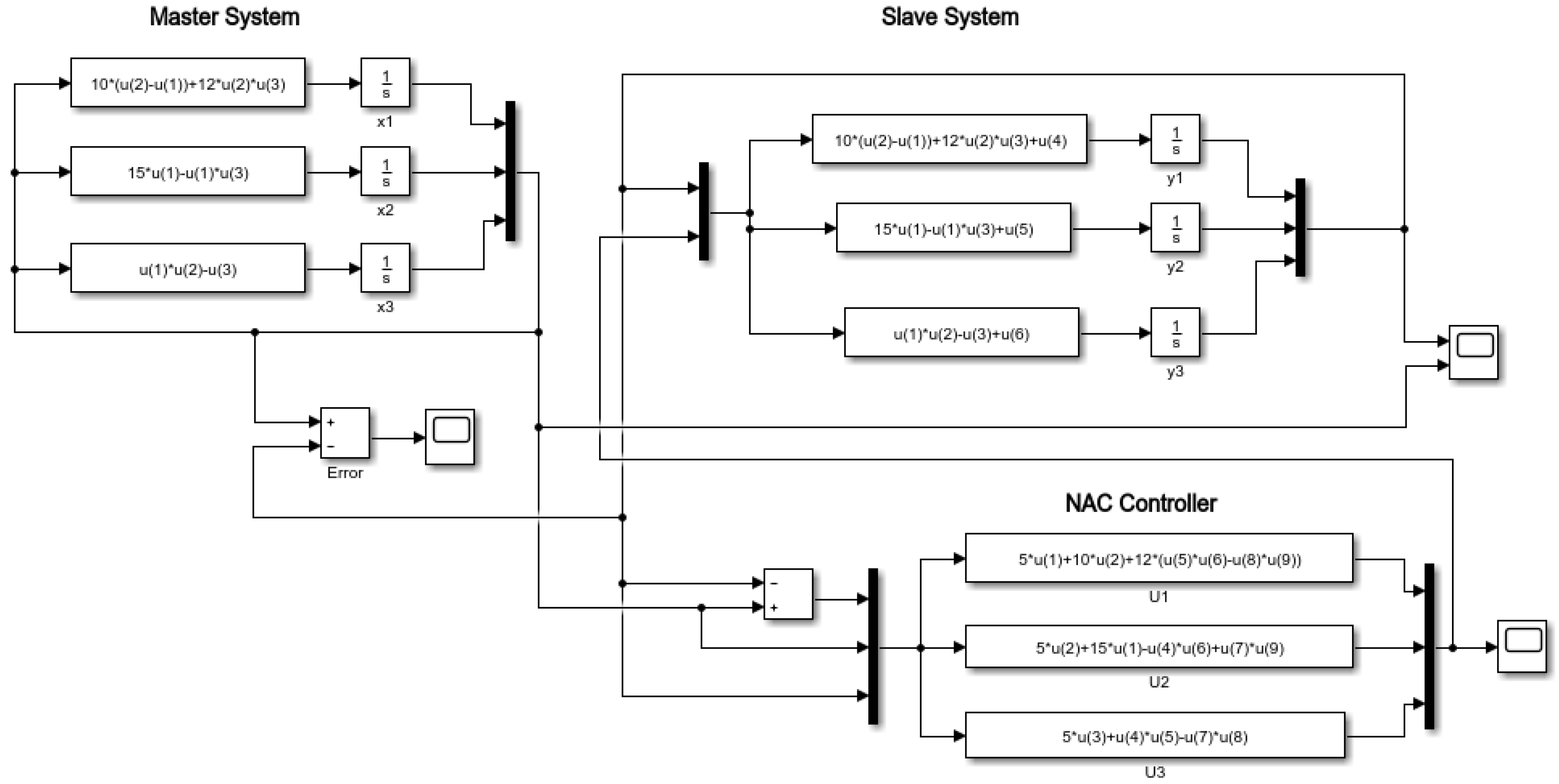
4. Application of the Nonlinear Active Control Method to Synchronize Chaotic Systems

Here we apply the nonlinear active control law (NAC) to three different synchronized chaotic systems.

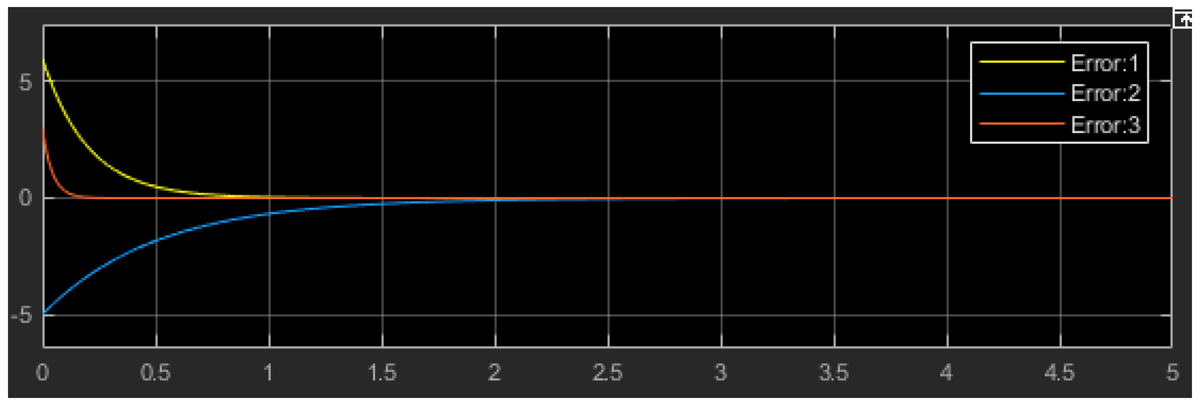
4.1. Application to the Bhalekar–Gejji Chaotic System

The master system is defined in Equation (1), and we define the slave system by
y 1 ˙ = ω y 1 y 2 2 + U 1 , y 2 ˙ = μ ( y 3 y 2 ) + U 2 , y 3 ˙ = α y 2 β y 3 + y 1 y 2 + U 3 ,
where y 1 , y 2 , and y 3 are the state variables of the slave system, and U 1 , U 2 , U 3 are the control laws to be determined before synchronization. We define the synchronization error e i as
e i = y i x i i = 1 , 2 , 3 .
The synchronization error Equation (15) must converge towards zero as defined in Equation (7). Thus, the problem of synchronization of two continuous chaotic systems transforms into controlling the error of the system to converge to zero. From Equations (1), (14), and (15), we obtain the dynamic synchronization error of the system as
e 1 ˙ = ω e 1 y 2 2 + x 2 2 + U 1 , e 2 ˙ = μ ( e 3 e 2 ) + U 2 , e 3 ˙ = α e 2 β e 3 + y 1 y 2 x 1 x 2 + U 3 .
Thus, Equation (16) can be rewritten in the form of
e ˙ = A e + B ( f ( y ) f ( x ) ) + U ( x , y ) ,
with A , B R n × m , f ( x ) , f ( y ) R n U R n are nonlinear functions and the control law. The system of Equation (17) therefore becomes
e 1 ˙ e 2 ˙ e 3 ˙ = ω 0 0 0 μ μ 0 α β e 1 e 2 e 3 + 1 0 0 0 0 0 0 0 1 y 2 2 x 2 2 0 y 1 y 2 x 1 x 2 + U 1 ˙ U 2 ˙ U 3 ˙ ,
where A = ω 0 0 0 μ μ 0 α β , B = 1 0 0 0 0 0 0 0 1   f ( y ) f ( x ) = y 2 2 x 2 2 0 y 1 y 2 x 1 x 2 .
The synchronization control law can be written according to Theorem 1 by
U = K ( y x ) B ( f ( y ) f ( x ) ) .
with the control parameter matrix. Equation (19) can be rewritten in the form K∈ R n × m
U 1 U 2 U 3 = k 11 k 12 k 13 k 21 k 22 k 23 k 31 k 32 k 33 e 1 e 2 e 3 1 0 0 0 0 0 0 0 1 y 2 2 x 2 2 0 y 1 y 2 x 1 x 2
To obtain synchronization, we rely on the condition of Theorem 1 and Inference 1 derived from the Lyapunov stability condition, which allows us to determine the elements k i j of the parameter matrix K. Therefore, we have
k 11 > ω , k 22 > μ , k 33 > β , k 12 = k 13 = k 21 = k 31 = 0 , k 23 = μ , k 32 = α .
This finally gives
U 1 = k 11 e 1 y 2 2 + x 2 2 , U 2 = k 22 e 2 + k 23 e 3 , U 3 = k 33 e 3 + k 32 e 2 + y 1 y 2 x 1 x 2 .
The control laws in Equation (22) satisfy the synchronization between the chaotic master–slave BG systems for all k i j in Equation (21). For this case, the initial conditions of the master system are x ( 0 ) = ( 1 , 5 , 0 ) ; those of the slave system are y ( 0 ) = ( 5 , 0 , 3 ) . Figure 4 illustrates the synchronization between ( x i y i ) states variables.
We observe from Figure 4 that each of the signals coming from the master and slave system start from different initial conditions and the control law is activated at 4 s ; the signal become synchronized at this point for different values of the control gain that satisfy Equation (21). In Figure 4a–d, the control gain values are ( k 11 , k 22 , k 33 ) = (5,5,5) and ( k 11 , k 22 , k 33 ) = (0,0,0), which satisfy Equation (21), and the synchronization is achieved. In Figure 4e,f, the control gain values are ( k 11 , k 22 , k 33 ) = (−2, −2, −2) for k 33 = 2 ; Equation (21) is not satisfied and synchronization is not achieved.
In Figure 5, we present the Simulink block diagram that describes the master–slave chaotic system and the NAC law. The simulation result is presented in Figure 6.

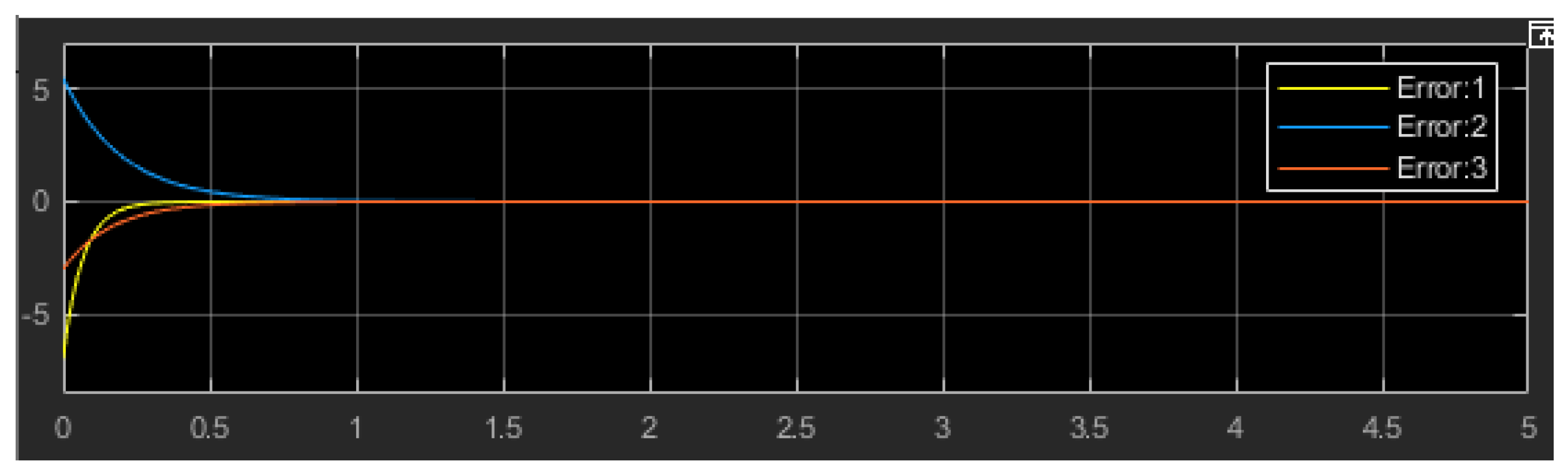
4.2. Application of the NAC Method to Chen’s System

The master system is described by Equation (2), and the slave system is given by Equation (23):
y 1 ˙ = a ( y 2 y 1 ) + U 1 , y 2 ˙ = ( c a ) y 1 y 1 y 3 + c y 2 + U 2 , y 3 ˙ = y 1 y 2 b y 3 + U 3 ,
where U 1 , U 2 , and U 3 are the control laws to be determined to obtain synchronization.
The application of the NAC method allows us to have the master–slave synchronization control law of the chaotic Chen systems by applying the same procedure; we obtain the following control parameters:
U 1 = k 11 e 1 + k 12 e 2 , U 2 = k 22 e 2 + k 21 e 1 x 1 x 3 + y 1 y 3 , U 3 = k 33 e 3 + x 1 x 2 y 1 y 2 ,
with
k 11 > a , k 22 > c , k 33 > b , k 13 = k 23 = k 31 = k 32 = 0 , k 12 = a , k 21 = c a .
The control law variables in Equation (24) satisfy the synchronization between master and slave systems for all k i j that satisfy Equation (25). For Chen’s system, the time series and trajectories x i y i , obtained by numerical simulation, are illustrated in Figure 7; at the start of the simulation, each signal starts from its initial condition until the controllers are activated at t = 5 s ; the systems became synchronized between the master and slave trajectories. Note that with the choice of the system parameters being fixed, the speed of convergence still depends on several factors, notably the choice of initial conditions and the choice of control gain k i j . In Figure 8, we present the Simulink diagram of the master–slave Chen’s system and NAC law to achieve synchronization. The simulation result of the errors of synchronization is presented in Figure 9; the errors converge to zeros at t .

4.3. Application to the 3D Chaotic Oscillator

The master system is described by Equation (3), and the slave system is given by Equation (26):
y 1 ˙ = b 1 ( y 2 y 1 ) + b 3 y 2 y 3 + U 1 , y 2 ˙ = b 2 y 1 y 1 y 3 + U 2 , y 3 ˙ = y 1 y 2 y 3 + U 3 ,
where U 1 , U 2 , and U 3 are the control laws to be determined.
The application of the NAC method allows us to have the master–slave synchronization control law of the chaotic 3D systems by applying the same procedure. We have the following control parameters:
U 1 = k 11 e 1 + k 12 e 2 b 3 ( x 2 x 3 y 2 y 3 ) , U 2 = k 22 e 2 + k 21 e 1 x 1 x 3 + y 1 y 3 , U 3 = k 33 e 3 + x 1 x 2 y 1 y 2 ,
with
k 11 > b 1 , k 22 > 0 , k 33 > 1 , k 13 = k 23 = k 31 = k 32 = 0 , k 12 = b 1 , k 21 = b 2 .
The control law Equation (27) satisfy the synchronization between master–slave systems for all k i j that satisfy Equation (28). For the simulations, the control parameters are ( k 11 , k 22 , k 33 ) = (2, 2, 2), which satisfy Equation (28). The initial conditions for the master system are x ( 0 ) = ( 1 , 0.5 , 0 ) and those of the slave system are y ( 0 ) = ( 0.5 , 1 , 3 ) . Figure 10 describes the time series x i y i and the errors synchronization of the trajectories of the master and slave systems of the 3D chaotic oscillator. In Figure 10a, master signals are marked in blue and response signals are in red. At the start of the simulation, each signal starts from its initial condition and then, when the controller is activated at t = 2 s , the trajectory of the slave system evolves until it completely matches the trajectory of the master system.
In Figure 11, we present the Simulink diagram of the master–slave 3D chaotic system and NAC law to achieve synchronization. The simulation result of the errors synchronization is presented in Figure 12; the errors converge to zeros at t = 0.5 .

5. Global Synchronization Scheme and Application to Secure Communication

In this section, we present the triple-cascade secure communication system configuration. Figure 13 is the Simulink block diagram of the secure communication system. This system is made of three large blocks: the transmitter block made up of the three master oscillators, the controllers block that allows synchronization between the master systems and the slave systems, and the receiver block, also made up of the three receiver oscillators. In the implementation of this communication system, in Figure 14, we consider a sinusoidal signal message as M ( t ) = 20 sin ( 2 π t ) . The masking technique considered here is a simple addition of signal; it consists of successively superposing on the information signal three signals coming from the three different chaotic oscillators. We have noted these signals X a ( t ) , X b ( t ) , and X c ( t ) , which come, respectively, from the 3D chaotic oscillator, the Chen chaotic system, and the BG chaotic system. Mathematically, the different output signals are taken as follows:
For the 3D chaotic oscillator described by Equation (3), we have: X a ( t ) = C 1 x a . For the Chen system described by Equation (2), we have: X b ( t ) = C 2 x b . For the BG system described by Equation (1), we have: X c ( t ) = C 3 x c , where C i represent the constant matrices of an appropriate dimension, representing the state variables measured and used for masking.

5.1. The Transmission Process

We have taken C i = [ 1 , 0 , 0 ] , i = 1, 2, 3. This means that we will only use a single variable at each chaotic oscillator to hide the message. The information signal is assumed to be one-dimensional; our masking is therefore carried out in three steps.
  • First step masking
The signal M ( t ) is masked by the output of the master 3D chaotic system X a ( t ) to generate the masked signal T 1 ( t ) .
T 1 ( t ) = M ( t ) + X a ( t ) = C 1 x a + M ( t ) = x a + M ( t ) .
  • Second step masking
The second step masking is carried out by once adding another chaotic signal to the signal T 1 ( t ) : T 2 ( t ) = X b ( t ) + T 1 ( t ) = X b ( t ) + C 1 x a + M ( t ) = C 1 x a + C 2 x b + M ( t )
From where T 2 ( t ) = C 1 x a + C 2 x b + M ( t )
T 2 ( t ) = x a + x b + M ( t ) .
  • Third step masking
At this stage, we once again add a third chaotic signal, namely X c ( t ) . Mathematically, we have:
T 3 ( t ) = X c ( t ) + T 2 ( t ) = X c ( t ) + C 1 x a + C 2 x b + M ( t ) = C 1 x a + C 2 x b + C 3 x c + M ( t ) This finally gives
T 3 ( t ) = x a + x b + x c + M ( t ) .
Figure 14 illustrates the difference between the initial message M ( t ) and the secure information signal T 3 ( t ) after the third masking step. As shown in Equation (31), three chaotic signals are represented by dynamic variables x a , x b , x c originating from the three different chaotic systems to mask the message from the transmitter side. This increases the complexity of the communication system and makes the message very difficult to be identified by an intruder. Our information signal M ( t ) underwent three successive masking steps. The signal T 3 ( t ) containing the information obtained after these three steps became more secure.

5.2. Recovery Process

To recover the transmitted message, the chaotic signal Y c ( t ) of the slave BG system is first subtracted from the received message T 3 ( t ) . Then, the chaotic signal of the slave Chen system Y b ( t ) and that of the slave 3D chaotic oscillator system Y a ( t ) are in turn subtracted to obtain the recovered information signal R(t). The output signal of the slave 3D chaotic system is described by Y a = C 1 y a . The output signals of the slave Chen’s system Equation (23) and BG system Equation (14) are, respectively, Y b = C 1 y b and Y c = C 1 y c . Therefore, we have R ( t ) = T 3 ( t ) Y c ( t ) Y b ( t ) Y a ( t ) .
R ( t ) = x a + x b + x c + M ( t ) y a y b y c .
Since synchronization controllers are designed to force the slave systems to synchronize with the master systems, lim t | y ( t ) x ( t ) | = 0 , the recovered information signal is equal to the original transmitted information signal M ( t ) . Figure 15 shows the recovered message and the original message after synchronization. We see the recovered signal R ( t ) converge to the original signal and synchronize correctly after a time of t = 0.5 s.

6. Robustness Evaluation of Chaotic System and Synchronization Scheme

Robustness evaluation involves assessing the stability, sensitivity to perturbations, and ability to maintain chaos or synchronization under uncertainties. The method of evaluation we consider here is parameter perturbation, noise resistance testing, and parameter variation.

6.1. Parameter Perturbation Analysis

Parameter perturbation analysis evaluates how small changes in system parameters affect the synchronization. It helps to determine the robustness of the synchronization scheme.
Consider a general nonlinear dynamical system
X ˙ = F ( X , P )
where X is the state variable and P is the system parameter. To evaluate this, we consider P ± Δ , where Δ is uncertainty. In Figure 16, we consider the 3D chaotic system and apply the uncertainties of Δ = 0.1 , 0.2, 0.3, and 0.4 to all parameters of the slave system. For different values of uncertainty Δ , the synchronization is maintained.

6.2. Noise Resistance Testing

Noise resistance testing evaluates how a synchronization maintains its dynamics under stochastic perturbations. Since real-world systems are subject to noise (e.g., thermal fluctuations, measurement errors), robustness requires that synchronization persists and remain stable.
X ˙ = F ( X , P ) + Γ ( t )
where F ( X , T ) is the dynamics system equation and Γ ( t ) is the noise term.
Here we consider noise term with finite amplitude:
Γ ( t ) = r a n d cos ( 40 t ) + r a n d sin ( 30 t ) + r a n d cos ( 20 t ) + r a n d sin ( 10 t ) + r a n d cos ( 5 t )
We introduce the perturbation term in the three states variable of the system as illustrated by (36).
x 1 ˙ = b 1 ( x 2 x 1 ) + b 3 x 2 x 3 + Γ , x 2 ˙ = b 2 x 1 x 1 x 3 + Γ , x 3 ˙ = x 1 x 2 x 3 + Γ ,
Figure 17 presents the noise margin and master–slave states variables of the 3D chaotic system. We can observe how synchronization is maintained and conclude the robustness of this synchronization scheme.

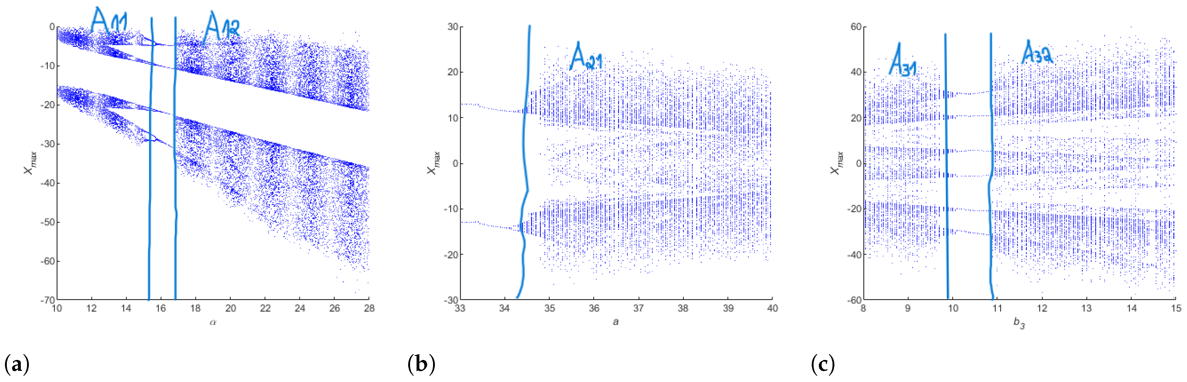
6.3. Bifurcation Diagram and Parameters Variation

A bifurcation diagram visualizes how a dynamical system’s behavior changes as a parameter varies, revealing transitions between periodic, chaotic, and stable states. It is a crucial tool for analyzing the robustness of chaos.
The approach is appealing due to the possibility of changing key parameters and maintaining chaotic behavior. In fact, if we will use a one-level system for which a set of key parameters are identified. Moreover, even if windows of chaos are generated by changing one parameter, the global parameter changing makes the system sensitive. This mean that we can pass from a chaotic condition to another behavior that is not chaotic. Indeed, this means that the sensitivity of a one-level system is critical.
Let us consider a multi-level chaotic system. A set of independent parameters that assure chaos are defined; this means that the real-time changing of the key parameters that are independent is maintained. A bifurcation diagram analysis of the considered system is reported. The three bifurcation diagrams refer to, respectively, the Bhalekar–Gejji system with the parameter a, Chen’s system with the parameter α , and the 3D chaotic system with the parameter b 3 ; these are shown in Figure 18. It is clearly evident that a great set of parameters guarantee the chaos of the global system, assuring security robustness. In fact, in this example, with A i j the set of chaotic parameters where i identify the system and j is the number of chaotic windows, it appears that the security level is augmented five times compared to considering only Chen’s system.

7. Conclusions

Data protection is a great challenge, and utilizing a chaotic system for encryption is a promising solution. This study presented a highly secure communication system based on the multi-level synchronization of three distinct chaotic systems: the Bhalekar–Gejji (BG) system, the Chen system, and a 3D chaotic oscillator. By employing the nonlinear active control (NAC) method, we successfully achieved robust synchronization between master and slave systems, ensuring stability through Lyapunov theory. The proposed triple-cascade masking technique significantly enhanced security by embedding the information signal within the chaotic outputs of all three systems, making unauthorized decryption exceedingly difficult without knowledge of each system’s dynamics. Numerical simulations and Simulink implementations confirmed the effectiveness of the synchronization process and the secure communication scheme. The results demonstrated that the transmitted signal becomes highly unpredictable and resistant to attacks and effectively concealed the original message. This approach not only improves upon traditional single-system chaos-based encryption but also offers a scalable framework for future enhancements, such as multi-signal masking or image encryption. Future research could explore the application of this method to multimedia security, including image and video encryption, as well as the integration of adaptive control techniques to further optimize synchronization performance under varying conditions. The proposed system holds significant promise for real-world secure communication applications, where high-level data protection is paramount.

Author Contributions

Methodology, K.Z.; Software, J.W.; Formal analysis, K.Z.; Writing—original draft, K.Z.; Writing—review & editing, L.F.; Supervision, L.F.; Funding acquisition, L.F. All authors have read and agreed to the published version of the manuscript.

Funding

This research received no external funding.

Data Availability Statement

Data are contained within the article.

Conflicts of Interest

The authors declare that they have no conflicts of interest.

References

  1. Feng, W.; Zhang, J.; Chen, Y.; Qin, Z.; Zhang, Y.; Ahmad, M.; Woźniak, M. Exploiting robust quadratic polynomial hyperchaotic map and pixel fusion strategy for efficient image encryption. Expert Syst. Appl. 2024, 246, 123190. [Google Scholar] [CrossRef]
  2. Feng, W.; Zhao, X.; Zhang, J.; Qin, Z.; Zhang, J.; He, Y. Image encryption algorithm based on plane-level image filtering and discrete logarithmic transform. Mathematics 2022, 10, 2751. [Google Scholar] [CrossRef]
  3. Yu, F.; Zhang, S.; Su, D.; Wu, Y.; Gracia, Y.M.; Yin, H. Dynamic Analysis and Implementation of FPGA for a New 4D Fractional-Order Memristive Hopfield Neural Network. Fractal Fract. 2025, 9, 115. [Google Scholar] [CrossRef]
  4. Pecora, L.M.; Carroll, T.L. Synchronization in chaotic systems. Phys. Rev. Lett. 1990, 64, 821. [Google Scholar] [CrossRef]
  5. Vaidyanathan, S.; Volos, C.; Pham, V.T.; Madhavan, K.; Idowu, B.A. Adaptive synchronization of chaotic systems with applications to secure communication. IEEE Trans. Cybern 2022, 52, 5009–5022. [Google Scholar]
  6. Khan, A.A.; Singh, J.P. Chaos-based image encryption using hybrid synchronization. Multimed. Tools Appl. 2023, 82, 5671–5690. [Google Scholar]
  7. Vaidyanathan, S. Adaptive chaotic synchronization of enzymes substrates system with ferroelectric behaviour in brain waves. Int. J. PharmTech Res. 2015, 8, 964–973. [Google Scholar]
  8. Fang, J.Q. Controlling Chaos and Developing High and New Technology; Atomic Energy Press: Beijing, China, 2022. [Google Scholar]
  9. Preishuber, M.; Hütter, T.; Katzenbeisser, S.; Uhl, A. Depreciating motivation and empirical security analysis of chaos-based image and video encryption. IEEE Trans. Inf. Forensics Secur. 2018, 13, 2137–2150. [Google Scholar] [CrossRef]
  10. Velamore, A.A.; Hegde, A.; Khan, A.A.; Deb, S. Dual cascaded fractional-order chaotic synchronization for secure communication with analog circuit realisation. In Proceedings of the 2021 IEEE Second International Conference on Control, Measurement and Instrumentation (CMI), Kolkata, India, 8–10 January 2021; pp. 1–6. [Google Scholar]
  11. Du, H.Y.; Zeng, Q.S.; Wang, C.H. Function projective synchronization of different chaotic systems with uncertain parameters. Phys. Lett. A 2008, 372, 5402–5410. [Google Scholar] [CrossRef]
  12. Feng, W.; Yang, J.; Zhao, X.; Qin, Z.; Zhang, J.; Zhu, Z.; Wen, H.; Qian, K. A Novel Multi-Channel Image Encryption Algorithm Leveraging Pixel Reorganization and Hyperchaotic Maps. Mathematics 2024, 12, 3917. [Google Scholar] [CrossRef]
  13. Feng, W.; Wang, Q.; Liu1, H.; Ren, Y.; Zhang, J.; Zhang, S.; Qian, K.; Wen, H. Exploiting Newly Designed Fractional-Order 3D Lorenz Chaotic System and 2DDiscrete Polynomial Hyper-Chaotic Map for High-Performance Multi-Image Encryption. Fractal Fract. 2023, 7, 887. [Google Scholar] [CrossRef]
  14. Liao, Y.; Lin, Y.; Li, Q.; Xing, Z.; Yuan, X. Lightweight Image Encryption Algorithm Using 4D-NDS: Compound Dynamic Diffusion and Single-Round Efficiency. IEEE Access 2025, 13, 74656–74666. [Google Scholar] [CrossRef]
  15. Yousef, A.; Arslan, M.; Jawad, A. A Lightweight Image Encryption Algorithm Based on Chaotic Mapand Random Substitution. Entropy 2022, 24, 1344. [Google Scholar]
  16. Tung-Tsun, L.; Shyi-Tsong, W. A Lightweight Keystream Generator Based on Expanded Chaos with a Counter for Secure IoT. Electronics 2024, 13, 5019. [Google Scholar] [CrossRef]
  17. Bonny, T.; Al Nassan, W.; Vaidyanathan, S.; Sambas, A. Highly-secured chaos-based communication system using cascaded masking technique and adaptive synchronization. Multimed. Tools Appl. 2023, 82, 34229–34258. [Google Scholar] [CrossRef]
  18. Singh, P.P.; Singh, J.P.; Roy, B.K. Synchronization and anti synchronization of Lu and Bhalekar-Gejji chaotic systems using nonlinear active control. Chaos Solitons Fractals 2014, 69, 31–39. [Google Scholar] [CrossRef]
  19. Bhalekar, S.B.; Gejji, V.D. A new chaotic dynamical system and its synchronization. In Proceedings of the International Conference on Mathematical Sciences in Honor of Prof. AM Mathai, Kerala, India, 17–19 January 2011; pp. 1–10. [Google Scholar]
  20. Chen, G.; Ueta, T. Yet another chaotic attractor. Int. J. Bifurc. Chaos 1999, 9, 1465–1466. [Google Scholar] [CrossRef]
  21. Shieh, C.S.; Hung, R.T. Hybrid control for synchronizing a chaotic system. Appl. Math. Model 2011, 35, 3751–3758. [Google Scholar] [CrossRef]
  22. Li, C.; Zhang, Y.; Wang, X.; Chen, G. AI-enhanced chaotic encryption for 5G networks. IEEE Trans. Commun. 2024, 72, 1–15. [Google Scholar]
  23. Occhipinti, L.; Fortuna, L.; Rizzo, A.; Frasca, M. Programmable Chaos Generator and Process for Use Thereof; STMicroelectronics S.r.l.: Agrate Brianza, Italy, 2005; p. 6842745. [Google Scholar]
  24. Vaidyanathan, S.; Alexander, P. A seven term novel 3-D chaotic system with three quadratic nonlinearities and its LABVIEW implementation. J. Coord. 2015, 1, 1–15. [Google Scholar]
  25. Bai, E.W.; Lonngren, K.E. Synchronization of two Lorenz systems using active control A seven term novel 3-D chaotic system with three quadratic nonlinearities and its LABVIEW implementation. Chaos Solitons Fractals 1997, 8, 51–58. [Google Scholar] [CrossRef]
  26. Bai, E.W.; Lonngren, K.E. Sequential synchronization of two Lorenz systems using active control. Chaos Solitons Fractals 2000, 11, 1041–1044. [Google Scholar] [CrossRef]
Figure 1. Numerical simulation of Bhalekar–Gejji chaotic system attractors: (a) x 1 x 2 plane; (b) x 1 x 3 plane; (c) x 2 x 3 plane; (d) 3D plot.
Electronics 14 02592 g001
Figure 2. Numerical simulation of Chen’s chaotic system attractors: (a) x 1 x 2 plane; (b) x 1 x 3 plane; (c) x 2 x 3 plane; (d) 3D plot.
Electronics 14 02592 g002
Figure 3. Numerical simulation of 3D chaotic system attractors: (a) x 1 x 2 plane; (b) x 1 x 3 plane; (c) x 2 x 3 plane; (d) 3D plot.
Electronics 14 02592 g003
Figure 4. Synchronization of the master–slave Bhalekar–Gejji system activated at t = 4 s time series x 1 y 1 , x 2 y 2 , x 3 y 3 , and errors ( e 1 , e 2 , e 3 ) for different values of control gain k i j : For (a,b): ( k 11 , k 22 , k 33 ) = (5,5,5); for (c,d): ( k 11 , k 22 , k 33 ) = (0,0,0); for (e,f): ( k 11 , k 22 , k 33 ) = ( 2 , 2 , 2 ) .
Electronics 14 02592 g004aElectronics 14 02592 g004b
Figure 5. Simulink block diagram of Bhalekar–Gejji master–slave system with the NAC control law.
Electronics 14 02592 g005
Figure 6. Error synchronization result from Simulink block diagram realization of the BG system.
Electronics 14 02592 g006
Figure 7. Synchronization of the master–slave Chen system activated at t = 5 s : (a) time series x 1 y 1 , x 2 y 2 , x 3 y 3 ; (b) errors ( e 1 , e 2 , e 3 ) for the control gain values ( k 11 , k 22 , k 33 ) = (−30, 30, 5).
Electronics 14 02592 g007
Figure 8. Simulink block diagram of master–slave Chen’s system with the NAC control law.
Electronics 14 02592 g008
Figure 9. Error synchronization result from Simulink block diagram realization of Chen’s system.
Electronics 14 02592 g009
Figure 10. Synchronization of 3D chaotic system master–slave activated at 0.5 s : (a) time series x 1 y 1 , x 2 y 2 , x 3 y 3 ; (b) errors ( e 1 , e 2 , e 3 ) synchronization and the control law are ( k 11 , k 22 , k 33 ) = (2, 2, 2).
Electronics 14 02592 g010
Figure 11. Simulink diagram synchronization of the master–slave 3D chaotic system.
Electronics 14 02592 g011
Figure 12. Error synchronization of the master–slave 3D chaotic system.
Electronics 14 02592 g012
Figure 13. Implementation of the triple-cascade chaotic synchronization setup with Simulink realization.
Electronics 14 02592 g013
Figure 14. The transmitted signal T 3 ( t ) in yellow after triple masking and the original message M ( t ) in blue.
Electronics 14 02592 g014
Figure 15. Recovered message M ( t ) in green and the transmitted original message in blue R ( t ) .
Electronics 14 02592 g015
Figure 16. Parameter perturbation analysis of NAC applied to the 3D chaotic system. The controllers are activated at t = 5 s : (a) Δ = + 0.1 ; (b) Δ = 0.2 ; (c) Δ = + 0.3 ; (d) Δ = 0.4 .
Electronics 14 02592 g016
Figure 17. Noise resistance testing: (a) noise; (b) time series x 1 blue, y 1 red; (c) x 2 blue, y 2 red; (d) x 3 blue, y 3 red.
Electronics 14 02592 g017
Figure 18. Bifurcation diagram: (a) Bhalekar–Gejji system; (b) Chen’s system; (c) 3D chaotic system.
Electronics 14 02592 g018
Disclaimer/Publisher’s Note: The statements, opinions and data contained in all publications are solely those of the individual author(s) and contributor(s) and not of MDPI and/or the editor(s). MDPI and/or the editor(s) disclaim responsibility for any injury to people or property resulting from any ideas, methods, instructions or products referred to in the content.

