Broken Wire Detection Based on TDFWNet and Its Application in the FAST Project

Abstract

This research proposes a wire-breakage detection method based on a Time-Domain Feature Weighted Network (TDFWNet) to address the challenging issue of wire-breakage detection in the feed source cabin drive cables of the Five-hundred-meter Aperture Spherical radio Telescope (FAST). The study begins with a temporal domain morphology analysis, revealing significant differences between wire-breakage signals and interference signals in key characteristic parameters such as waveform factor, pulse factor, and kurtosis. These parameters are thus employed as the basis for feature input, and their corresponding feature probabilities are calculated to provide prior feature weights for the model. The TDFWNet model integrates the feature learning capability of a Convolutional Neural Network (CNN) with temporal domain feature analysis using the feature probabilities derived from key temporal domain characteristic parameters as weight inputs to enhance the sensitivity and recognition accuracy of wire-breakage signals. Furthermore, the research team has developed a data augmentation method based on Feature-Constrained Dynamic Time Warping (FCDTW). This method processes the original wire-breakage signals to generate high-quality augmented data, thereby improving the model’s ability to recognize wire-breakage signals. Ultimately, the TDFWNet outperforms traditional CNN models by 1.5%, 2.0%, 1.8%, and 16.6% in precision, recall, F1 score, and accuracy, respectively. In practical engineering applications, this method demonstrated excellent stability and practicality in three domestic FAST drive cable-bending fatigue tests. The detected suspected wire-breakage signals were highly consistent with the results of post-fatigue test disassembly inspections, effectively supporting the wire-breakage detection requirements in actual engineering scenarios.

1. Introduction

The steel wire is a primary component of the drive cable for the FAST (Five-hundred-meter Aperture Spherical radio Telescope) feed cabin. Figure 1a presents the panoramic view of FAST, while Figure 1b illustrates the feed cabin. The mechanical properties of the entire drive cable system are significantly influenced by the health condition of each steel wire. In practical engineering applications, the occurrence of broken wires within the cable is often inevitable. If these broken wires cannot be promptly and effectively detected, they pose considerable risks to the safety of the engineering structure [1,2,3]. Therefore, it is essential to develop a detection method that can timely identify broken wires, thereby enabling a more accurate assessment of the drive cable performance during tests and ensuring the safe operation of FAST in actual engineering applications.

The current methods for broken wire detection can be broadly categorized into manual identification and machine identification. Manual identification refers to the process where the occurrence of broken wires can be determined through certain means, but it requires human observation and judgment of the data. In contrast, machine identification involves the use of fixed algorithms and neural networks, among other methods, to recognize broken wires at the software level without human intervention. The manual identification methods mainly include the pressure sensor method, magnetic detection method, acoustic emission method, and fiber Bragg grating (FBG) sensor method. Among these, the pressure sensor method estimates the internal condition of the rope by measuring the tensile force. Although this method can provide certain information, it cannot reliably distinguish broken wires from other types of internal damage. Additionally, the installation of sensors is complex, and the application scope is limited [4,5,6]. The fundamental principle of magnetic detection is to determine whether internal wire breaks have occurred based on the changes in magnetic flux within magnetized metals [7,8,9]. Zhang et al. proposed a method for quantitatively characterizing the axial wire break width of a rope body through magnetic flux leakage detection [10]. Ni et al. identified and quantified wire break regions in bridge cables using a magnetic flux detection method and validated the effectiveness of this method through finite element analysis and experimental verification [8]. Additionally, some researchers have utilized the self-magnetization of ferromagnetic materials in the geomagnetic field to detect defects in wire ropes using the self-magnetic flux leakage method [11]. However, these methods are susceptible to electromagnetic interference, and the magnetic pole materials are prone to chemical corrosion, which limits their feasibility for long-term application. Acoustic emission detection, on the other hand, identifies damage by detecting the acoustic waves generated during the breaking or corrosion process of wire ropes [12,13,14]. Li et al. designed a novel acoustic emission (AE) signal segmentation algorithm, which enhanced the effectiveness of AE technology through noise filtering and signal extraction [15]. Li investigated and proposed a shell-type AE monitoring method for detecting various damage sources in cables including wire breaks, corrosion, and fatigue. The study also established the relationship between the thickness of the high-density polyethylene shell and the AE transmission coefficient as well as circumferential AE attenuation models for three different types of cables. Based on these models, a sensor layout method was proposed to effectively monitor various cable damage with the minimum number of sensors [16]. Although AE methods have demonstrated high detection accuracy in laboratory settings, they are highly sensitive to noise and require stringent environmental conditions for practical applications [17]. Yu et al. embedded an FBG vibration sensor into the central wire of a steel strand under prestress, thereby fabricating a self-sensing steel strand capable of accurately identifying the fracture of each wire. The study demonstrated that the intensity of the wire-breakage signal is independent of the location of the FBG measurement point but is related to the position, degree, and region of damage in the ordinary wires [18]. This research effectively validated the feasibility of utilizing FBG vibration sensors to monitor the health condition of stay cables and detect wire fractures.

In recent years, with the development of artificial intelligence and deep learning technologies, machine recognition methods have gradually demonstrated their advantages in the field of broken wire detection. Xue et al. proposed a method for assessing the damage condition of cable wires based on a Deep Reference Autoencoder Convolutional Neural Network model, which improved the efficiency of broken wire detection [19]. Han et al. conducted a diagnosis of internal broken wires in steel ropes using a Residual Neural Network model. Their research results indicated that compared with traditional neural network methods such as backpropagation, ResNet exhibited superior performance in detecting broken wires in steel ropes [20]. In contrast, the Support Vector Machine model has shown more remarkable performance in broken wire detection, but its high computational complexity limits its application in practical detection [21,22,23]. Wang et al. significantly enhanced the accuracy and efficiency of transmission line strand breakage detection by introducing deformable convolution modules and hybrid attention convolution modules into an improved YOLOv8 network model, and employing the Inner-SIoU loss function, achieved an average detection accuracy of 92.5%. However, the study did not verify the long-term stability and scalability of the model in practical power system operation and maintenance [24]. As a powerful deep learning model, CNN is capable of automatic extraction and identification of complex signal features, and thus, has gradually become an important tool for broken wire signal detection. Zhang et al. proposed a quantitative identification method based on wavelet transform and CNN that converts magnetic flux leakage signals into time-frequency images for broken wire recognition, thereby significantly improving the detection accuracy [25]. Zhu et al. achieved high-precision detection of broken wires in steel strands by combining CNN with a self-sensing steel strand that embeds FBG vibration sensors pre-compressed into the central wire of the steel strand. The test results showed that the accuracy of broken wire detection reached 99.77%, with an average error of 0.38% in predicting the location of broken wires, and the model successfully detected all 118 real broken wires [26]. This work has validated the feasibility of using artificial intelligence for the precise identification of broken wire signals. Liu et al., building on the work of Zhu et al., proposed a novel method for steel wire breakage detection based on an improved external FBG vibration sensor and CNN, achieving accuracies of 98.49% and 96.79% in pulse and step signal interference tests, respectively. Nevertheless, the method exhibits limited adaptability to steel wire ropes with smaller diameters or under vibration interference conditions and has certain limitations in the practical application of broken wire detection in FAST drive cables [27].

The drive cables of the FAST feed cabin are composed of 384 steel wires with diameters ranging from ø1 to ø2.7 mm, which are much finer than conventional steel strands. Combined with various interference signals in the environment, identifying broken wire signals is particularly challenging. To address this issue, based on the research of Zhu et al. [28,29,30], this study proposes an innovative network model, namely TDFWNet. This model integrates time-domain features with CNN to identify broken wire signals from vibration signals collected by external FBG vibration sensors. TDFWNet not only inherits the powerful feature learning capability of CNN but also significantly enhances the model’s sensitivity and recognition accuracy for broken wire signals by incorporating feature probabilities calculated from key time-domain feature parameters as weighted inputs. Additionally, it improves the ability to distinguish interference signals.

The remainder of this paper is organized as follows: The section “Theory and Methods” delves into the time-domain feature analysis of broken wire signals, introduces the basic principles of CNN, and discusses the application principles of the Dynamic Time Warping (DTW) algorithm in data augmentation. The section “Time-Domain Feature Weighted Network” provides a detailed description of the dataset preparation process, the data augmentation method based on FCDTW, and the architecture design and performance evaluation of the TDFWNet model. The section “Engineering Application” focuses on the practical application of TDFWNet in broken wire detection of the FAST feed cabin drive cables bending fatigue test, including the drive cable structure and fatigue test design, detection methods, data acquisition procedures, and bending fatigue test results. Finally, the “Conclusions” section summarizes the main findings and contributions of this study and highlights the significant advantages and broad application prospects of TDFWNet in the field of broken wire detection.

2. Theory and Methods

2.1. Time-Domain Feature Analysis

Before the construction of the TDFWNet, we conducted a time-frequency analysis of the broken wire signals of the FAST drive cable collected in the experiment (the specific experiment is detailed in Section 3.1). These signals were compared with the interference signals generated during the bending fatigue test of the drive cable. The interference signals were caused by resonance between the drive cable and the experimental system during repeated bending. The results revealed that the differences between the two types of signals in the frequency domain were minimal, as shown in Figure 2, where both signals occupied the entire frequency band. Therefore, it was challenging to distinguish between them through frequency-domain analysis. However, upon analyzing the time-domain waveforms of the broken-wire and interference signals, distinct differences were observed. The broken wire signal exhibited an initial increase in oscillation followed by a decrease, presenting an overall trend of fluctuation attenuation. In contrast, the interference signal demonstrated a sudden oscillation attenuation with a sharp change in amplitude at the initial moment that gradually became more stable over time, as illustrated in Figure 3.

To further investigate the differences in the time-domain characteristics between the broken wire signals and the frequently occurring interference signals in bending fatigue tests, we selected eight characteristic parameters that represent the distribution of signal time-domain features: peak factor, waveform factor, pulse factor, skewness, kurtosis, variance, root mean square, and rectified average value. We conducted a time-domain feature analysis of the broken wire signals and interference signals using these parameters. The final analysis results are presented in Figure 4.

The analysis of the results from the figure indicates that the differences between broken wire signals and interference signals are particularly pronounced in three key characteristic parameters: waveform factor, pulse factor, and kurtosis. The calculation formulas for these three parameters are given in Equations (1)–(3), where x_i represents the amplitude of the signal at the i-th moment, and N denotes the length of the signal. The median value of the waveform factor of broken wire signals is approximately 1.62, which is higher than that of interference signals (1.32). This suggests that the waveform of broken wire signals exhibits more singular points and deviates more from a sinusoidal waveform. In terms of the pulse factor, the median value of broken wire signals is close to 6.3, while that of interference signals is around 4.1. This indicates that broken wire signals contain more pulse-like transient components, which may correspond to the instantaneous impacts generated at the moment of wire breakage. The difference in kurtosis is also significant. The median kurtosis of broken wire signals ranges from 6 to 10, whereas that of interference signals lies between 3 and 5. This reflects that the waveform of broken wire signals exhibits sharper peaks, which is a typical characteristic of transient impact signals and is highly consistent with the instantaneous vibrations generated by broken-wire faults.

$$\mathrm{y}=\mathrm{N}{\displaystyle \frac{\sqrt{\frac{1}{\mathrm{N}}{\sum }_{\mathrm{i}=1}^{\mathrm{N}}{\mathrm{x}}_{\mathrm{i}}^2}}{{\sum }_{\mathrm{i}=1}^{\mathrm{N}}|{\mathrm{x}}_{\mathrm{i}}|}}$$

(1)

$$\mathrm{y}=\mathrm{N}{\displaystyle \frac{\max (\left|{\mathrm{x}}_{\mathrm{i}}\right|)}{{\sum }_{\mathrm{i}=1}^{\mathrm{N}}|{\mathrm{x}}_{\mathrm{i}}|}}$$

(2)

$$\mathrm{y}={\displaystyle \frac{{\left(\frac{1}{\mathrm{N}}{\sum }_{\mathrm{i}=1}^{\mathrm{N}}{\mathrm{x}}_{\mathrm{i}}^4\right)}^{1/4}}{\sqrt{\frac{1}{\mathrm{N}}{\sum }_{\mathrm{i}=1}^{\mathrm{N}}({\mathrm{x}}_{\mathrm{i}}-\bar{\mathrm{x}}{)}^2}}}$$

(3)

Accordingly, based on the aforementioned differences in time-domain characteristics, this study proposes to embed waveform factor, pulse factor, and kurtosis as prior knowledge into a CNN, thereby constructing the TDFWNet model. Moreover, the model is provided with prior feature weights for broken wire identification, which enhances the model’s sensitivity and recognition accuracy for broken wire signals while simultaneously strengthening its ability to distinguish interference signals.

2.2. Convolutional Neural Network

CNN is the core of TDFWNet, originating from the field of computer vision. Its typical architecture comprises an input layer, convolutional layers, pooling layers, and fully connected layers. The convolutional layers are responsible for extracting local features, while the pooling layers reduce the dimensionality of the feature maps to mitigate the risk of overfitting. The fully connected layers integrate the extracted features to achieve the final classification. The convolution operation supports three modes: same, full, and valid, as illustrated in Figure 5. The number of convolutional kernels determines the depth of the output tensor, which in turn affects the network’s capacity to represent complex features.

The loss function of the model is generally chosen as categorical_crossentropy, which is suitable for multi-class classification problems. The expression of this loss function is shown in Equation (4).

$$\mathit{Loss} =-{\displaystyle \mathit{\sum }}_{i=1}^{\begin{array}{c}output\\ size\end{array}}{y}_i·log{\widehat{y}}_i$$

(4)

The optimizer is capable of finding the parameters that minimize the loss function. The Adam optimizer is commonly employed in the model. It can integrate the gradients of all samples, facilitating the search for the global optimal solution. Moreover, it retains the information of previous gradients, enabling gradient propagation [31,32]. The principal formula is as follows:

$${\theta }_{t+1}={\theta }_t-{\displaystyle \frac{\eta }{\sqrt{{\widehat{v}}_t}+ϵ}}{\widehat{m}}_t$$

(5)

In regression models, the activation function is generally chosen as ReLU. In classification models, the activation function is typically selected as Sigmoid. Their expressions are as follows:

$$\mathrm{R}\mathrm{e}\mathrm{l}\mathrm{u}\left(\mathrm{x}\right)=\left\{\begin{array}{l}\mathrm{x},\mathrm{x}\ge 0\\ 0,\mathrm{x}<0\end{array}\right.\Delta \mathsf{\epsilon }={\displaystyle \frac{\Delta \mathrm{l}}{\mathrm{l}}}={\displaystyle \frac{\sqrt{{\mathrm{l}}^2+{\mathrm{y}}^2}-\mathrm{l}}{\mathrm{l}}}$$

(6)

$$\mathrm{S}\mathrm{i}\mathrm{g}\mathrm{m}\mathrm{o}\mathrm{i}\mathrm{d}\left({\mathrm{z}}_{\mathrm{i}}\right)={\displaystyle \frac{1}{1+{\mathrm{e}}^{{-\mathrm{z}}_{\mathrm{i}}}}}$$

(7)

In Equation (4), z_i represents the output value of the i-th node. Through this function, the classification results can be transformed into a probability distribution with values ranging from 0 to 1 and summing to 1, thereby achieving classification.

CNN implicitly learns to extract features from data without requiring explicit feature extraction [33]. However, in the task of broken wire signal recognition, relying solely on implicit feature extraction by CNN may fail to fully utilize the known prior information of temporal domain features. Therefore, we propose TDFWNet, which integrates the powerful feature learning capability of CNN with temporal domain feature analysis. By using the feature probabilities calculated from key temporal domain feature parameters as weights, TDFWNet enhances the model’s sensitivity to broken wire signals. In this manner, TDFWNet not only inherits the advantages of CNNs but also leverages the significant differences in temporal domain features between broken wire signals and interference signals, thereby achieving more efficient broken wire signal recognition.

2.3. Dynamic Time Warping

DTW is a classical algorithm for solving the problem of nonlinear alignment of time series. Its core lies in constructing the optimal alignment path between two sequences through dynamic programming, minimizing the cumulative distance to eliminate temporal offsets [34,35]. Given two sequences X = (x₁,…,x_m) and Y = (y₁,…,y_n), DTW defines a cumulative distance matrix D(i,j) with the following recursive formula:

$$\mathrm{D}(\mathrm{i},\mathrm{j})=|{\mathrm{x}}_{\mathrm{i}}-{\mathrm{y}}_{\mathrm{j}}|+\min \left\{\mathrm{D}(\mathrm{i}-1,\mathrm{j}),\mathrm{D}(\mathrm{i},\mathrm{j}-1),\mathrm{D}(\mathrm{i}-1,\mathrm{j}-1)\right\}$$

(8)

The final DTW distance is D(m,n), which reflects the global similarity between the two sequences. This algorithm ensures the physical significance of the alignment through path constraints (boundary conditions, monotonicity, and continuity) and is widely applied in speech recognition and industrial signal analysis.

$${\mathrm{s}}_{\mathrm{n}\mathrm{e}\mathrm{w}}\left(\mathrm{k}\right)=\mathsf{\alpha }·{\mathrm{s}}_1\left({\mathrm{p}}_1\right)+(1-\mathsf{\alpha })·{\mathrm{s}}_2\left({\mathrm{p}}_2\right)$$

(9)

In the context of data augmentation tasks, two time-series samples can be randomly selected to compute their DTW path. Subsequently, interpolation is performed on the two sequences based on this path to generate new sequences with the interpolation formula given in Equation (9). Here, s₁ and s₂ are the original sequences, p₁ and p₂ are the corresponding points in the DTW path, and $\alpha$ is the interpolation coefficient, which is typically set to 0.5 to ensure that the new sequence is the average of the two original sequences. Finally, the augmented signal after interpolation is downsampled using dynamic resampling techniques. Through this approach, the original signal characteristics of the synthesized signal can be fully preserved, and more representative and diverse training data can be generated, thereby enhancing the performance of the TDFWNet model.

3. Time-Domain Feature Weighted Network

3.1. Dataset Preparation

To construct the training dataset for the TDFWNet model, the present study conducted breaking tests on four FAST drive cables to obtain the broken wire signal data. The tests were performed at the Mechanics and Structural Engineering Laboratory of the National Center for Safety Science of Materials Service at the University of Science and Technology Beijing. An MTS 244S ± 2500 kN dual-rod dynamic actuator, manufactured by MTS Systems Corporation in the United States, was employed. To ensure the safety of the testing process, a displacement-controlled loading mode was adopted, with a loading rate of 4 mm/min, which was carried out at a uniform, slow, and stable pace. The tensile force was recorded in real time, with the rate of force increase controlled to be no more than 0.5% of the minimum breaking force per second (approximately 9 kN/s). For signal acquisition, a fiber Bragg grating vibration sensor was used with a sampling frequency set at 100 Hz.

Ultimately, the experiment yielded 23 sets of complete and valid broken wire signal data, which provided a crucial foundation for subsequent data augmentation and training of the TDFWNet model. Figure 6 presents the pictures of the experimental site.

3.2. FCDTW Data Augmentation

During the data augmentation process, we introduced an improved DTW method, namely FCDTW. FCDTW initially computes the alignment path through Dynamic Time Warping to perform nonlinear alignment of the signals. Subsequently, it integrates the signals using an interpolation function. We set the interpolation coefficient at 0.5 to ensure that the new sequence obtained through interpolation is the average of the two original sequences. The augmented data are then uniformly resampled to preserve their original characteristics. Additionally, amplitude scaling and time-shifting are incorporated to simulate real-world operational variations. The critical time-domain feature constraints are reflected in the strict control of the waveform factor, pulse factor, and kurtosis of the broken wire segment (as shown in Figure 2b for the characteristic segment of the broken wire signal). Specifically, a sample is considered valid only when the waveform factor, pulse factor, and kurtosis of the generated signal match those of the broken wire signal. This constraint ensures the key physical characteristics of the broken wire signal are maintained while preserving the diversity of the generated data, thereby guaranteeing the rationality of the signal morphology. The data augmentation technique route of FCDTW is illustrated in Figure 7.

The generated signal data are saved in xlsx files, with each file containing 200 data points that cover the main feature regions of the broken wire signals and are labeled with 1 for broken wire signals and 0 for unbroken wire signals. To evaluate the quality of the augmented data generated by FCDTW, we compared it with three other widely used data augmentation methods, namely DTW, Generative Adversarial Network (GAN), and Variational Autoencoders (VAEs). These 4 methods were employed to augment 23 sets of original broken wire signals and interference signals (unbroken wire signals) collected from bending fatigue tests, with each method generating 2990 sets of broken and unbroken wire signals. Subsequently, the t-SNE algorithm was utilized for dimensionality reduction and clustering analysis to visually assess the consistency and separability of the augmented data relative to the original data, thereby evaluating the effectiveness of data augmentation [36].

The t-SNE analysis results in Figure 8 demonstrate that the data generated by FCDTW exhibit superior performance in preserving the characteristics of the original data. Specifically, the enhanced data for broken and unbroken wires by FCDTW cluster closely around the original data, presenting a well-defined clustering structure with clear boundaries between the two categories. DTW, in contrast, shows slightly inferior clustering compactness for unbroken wire data, with some data points deviating from the original distribution. The broken wire data generated by GAN are not tightly clustered and exhibit a significant deviation in distribution, while the broken wire data generated by VAE are loosely clustered with low overlap with the original data. Figure 9 presents examples of some original data and augmented data to intuitively demonstrate the effect of data augmentation.

Overall, the proposed FCDTW outperforms other methods in terms of feature preservation, clustering compactness, and class discrimination. This indicates that the enhanced data generated by FCDTW are of higher quality and are more conducive to improving the model’s ability to recognize broken wire signals.

3.3. Model Architecture and Evaluation

TDFWNet is a hybrid deep learning architecture that integrates CNN with time-domain features and is designed to enhance the robustness and accuracy of broken wire signal recognition. The model input is a one-dimensional time-series signal with a shape of (200,1). Through multi-layer convolution and pooling operations, spatiotemporal features are extracted. The number of convolutional kernels progressively increases with each layer, and Dropout layers are introduced to suppress overfitting. The specific parameter configurations are detailed in

Table 1. Model parameter configuration.

	Name	Dimension of Output Value
Convolution	Conv1D	(None, 198, 32)
	MaxPooling1D	(None, 99, 32)
	Conv1D_1	(None, 97, 64)
	Dropout	(None, 97, 64)
	MaxPooling1D_1	(None, 48, 64)
	Conv1D_2	(None, 46, 128)
	Dropout_1	(None, 46, 128)
	MaxPooling1D_2	(None, 23, 128)
	Conv1D_3	(None, 21, 256)
	Dropout_2	(None, 21, 256)
	MaxPooling1D_3	(None, 10, 256)
Flatten	Flatten	(None, 2560)
Dense	Dense	(None, 256)
	Dense_1	(None, 128)
	Dense_2	(None, 200)

.

After feature extraction, the model introduces a key innovation point—a feature probability weighting module. The calculation formula for the feature probability is given by the following:

$$P_{feature}=\alpha ·P_{waveform}+\beta ·P_{kurtosis}+\gamma ·P_{pulse}$$

(10)

In the formula, $P_{waveform}$, $P_{kurtosis}$, and $P_{pulse}$ represent the broken wire probability values corresponding to the waveform factor, kurtosis, and impulse factor of the current feature segment (the continuous data segment where the broken wire probability exceeds 0.5), respectively. These feature segments are determined by the CNN after feature learning and recognition of the original input signal, and they provide the basic input for the subsequent calculation of feature probabilities. Their broken wire probability values are confined to the range (0, 1). Based on the time-domain feature analysis in Section 2.1, the weights for these three characteristics are set to α = 0.6, β = 0.3, and γ = 0.1. Equation (11) is the calculation formula for $P_{waveform}$, $P_{kurtosis}$, and $P_{pulse}$, where x is the time-domain characteristic value of the current feature segment and $min,{ Med}_{lower},{ Med}_{upper},max$ are the minimum value, lower median, upper median, and maximum value of the three time-domain feature values of the broken wire signal, respectively, as detailed in

Table 2. Minimum, lower quartile, upper quartile, and maximum values of three time-domain features of broken wire signals.

Time-Domain Features	Minimum Value	Lower Quartile	Upper Quartile	Maximum Value
Waveform factor	1.443633	1.529352	1.720721	1.894116
Kurtosis	4.654313	6.279180	9.748393	14.907855
Pulse factor	4.219765	5.473978	7.184436	9.000339

.

$$\left\{\begin{array}{ll}0.5-0.5·{\displaystyle \frac{\mathit{min}-x}{\mathit{max}-min}},& x<min\\ 0.5+0.5·{\displaystyle \frac{x-min}{{Med}_{lower}-min}},& \mathit{min}\le x<{Med}_{lower}\\ 1.0,& {Med}_{lower}\le x\le {Med}_{upper}\\ 1.0-0.5·{\displaystyle \frac{x-{Med}_{upper}}{\mathit{max}-{Med}_{upper}}},& {Med}_{upper}<x\le max\\ 0.5-0.5·{\displaystyle \frac{x-max}{\mathit{max}-min}},& x>max\end{array}\right.$$

(11)

The final output is computed via a weighted fusion mechanism, with the formula as follows:

$$P_{final}=w·P_{CNN}+(1-w)·P_{feature}$$

(12)

where $P_{CNN}$ denotes the probability of broken wire predicted by the CNN and $w$ is the weight coefficient that determines the proportion of CNN prediction and feature probability.

Multiple training experiments have demonstrated that TDFWNet is highly sensitive to the learning rate, enhancement factor, and weight coefficient. As shown in Figure 10a–c, when the learning rate is set to 0.0009, the data augmentation factor is 130 and $w$ = 0.8; the gap between the training accuracy and validation accuracy of the model is minimized, while both reach relatively high values. This indicates that the model achieves the best balance between fitting performance and generalization ability under these conditions, thereby maximizing its capability to identify broken wire data. The final structure of the TDFWNet model is illustrated in Figure 11.

$$Precision={\displaystyle \frac{TP}{TP+FP}}$$

(13)

$$Recall={\displaystyle \frac{TP}{TP+FN}}$$

(14)

$$F1=2\times {\displaystyle \frac{Precision\times Recall}{Precision+Recall}}$$

(15)

$$Accuracy={\displaystyle \frac{TP+TN}{TP+TN+FP+FN}}$$

(16)

Finally, the performance of the TDFWNet model proposed in this paper was compared with the CNN proposed by Liu et al. [27]. through ten independent training experiments. The datasets used for evaluation were all augmented by a factor of 130, with 25% of the data reserved as the test set and the remaining 75% utilized for training to validate the accuracy and robustness of the models. The evaluation metrics employed were precision, recall, F1 score, and accuracy; the calculation formulas are given in Equations (13)–(16). In these equations, TP, FN, TP, and TN represent false positives, false negatives, true positives, and true negatives, respectively.

The comparative analysis results (Figure 10d) indicate that TDFWNet outperforms the CNN model constructed by Liu et al. in key performance metrics including precision, recall, F1 score, and accuracy. Specifically, after 10 training iterations, TDFWNet achieved an average precision of 98.5%, an average recall of 97.2%, an average F1 score of 97.9%, and an average accuracy of 91.5%, which are 1.5%, 2.0%, 1.8%, and 16.6% higher than those of the CNN model, respectively. The error bars in the figure demonstrate that TDFWNet has a relatively narrow range of error in all metrics, indicating a more stable performance. In contrast, the 1DCNN exhibits longer error bars, particularly for recall and accuracy, suggesting significant fluctuations in its performance. Therefore, it can be concluded that TDFWNet not only performs better in all metrics but also exhibits more stable and reliable performance.

The performance enhancement is attributed to the unique feature-weighted mechanism of TDFWNet. This mechanism enables the model to integrate the deep features automatically extracted by CNN and incorporate prior feature probabilities to guide the training process. Moreover, the real FAST-driven broken wire signal dataset utilized by TDFWNet exhibits significant differences in amplitude and duration compared with the broken wire signals of ordinary steel strands, as shown in Figure 12. These differences are also critical factors contributing to the substantial improvement in model performance. The hybrid architecture demonstrates superior robustness and adaptability in processing complex temporal signals, offering a novel technological paradigm for industrial signal analysis. It is particularly suitable for scenarios with imbalanced feature distributions or significant noise interference and holds broad application prospects.

4. Engineering Application

To verify whether the performance of the domestic drive cable meets the actual usage requirements of the FAST project, in addition to complying with relevant national standards such as the GB/T 20118-2017, a comprehensive evaluation through specifically designed fatigue testing methods is also required [37].

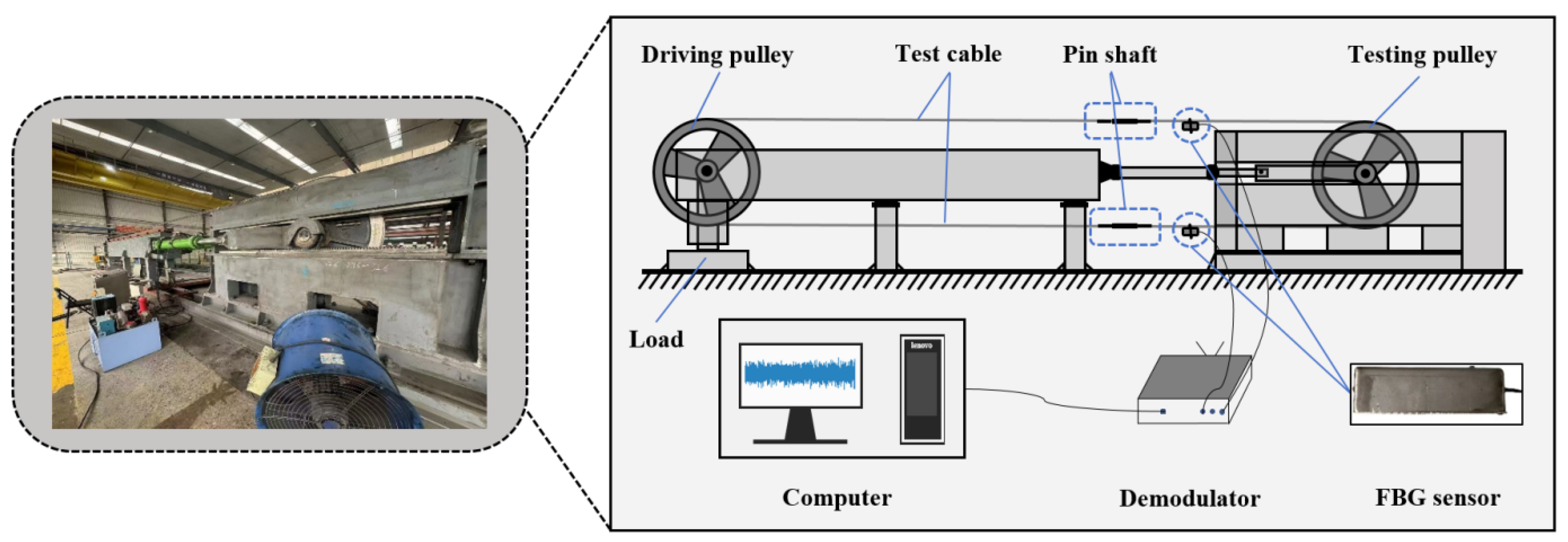
4.1. Structure of the Drive Cable and Fatigue Test Design

The drive cable adopts a ZBB 10×K26WS-EPIWRC structure with a strand configuration of 1 − 5 − 5 + 5 − 10, as shown in Figure 1c. The outer strands of the drive cable are composed of 1×K26WS, consisting of 26 steel wires closely arranged, which endows the cable with high fatigue resistance. The core structure is a composite configuration of CFRC8 × K7, including 8 × K7, 8 × 7, and 1 × 9W, providing reliable support for the outer strands. The nominal diameter of the cable is 46.00 mm, with the steel wire diameter ranging from 1.00 mm to 3.00 mm. The linear density is 9.99 kg/m, and the minimum breaking force reaches 1800 kN. To achieve precise tension transmission, the ends of the drive cable are connected through casting with anchorages. The anchorages are made of high-strength cast steel (35CrMo) with a tensile strength of no less than 960 MPa.

The experiments were conducted in the laboratory of Anshan Iron and Steel Wire Rope Co., Ltd. The design of the fatigue tests was based on the standard GB/T 12347-2008 and the specific requirements proposed by the National Astronomical Observatories of the Chinese Academy of Sciences [38]. The testing apparatus consisted of a testing pulley, a driving pulley, a test cable, a pin shaft, a demodulator, and an FBG vibration sensor, as shown in Figure 13. The diameter of the testing pulley was 2.6 m and that of the driving pulley was 2.8 m, with a center-to-center distance of 12.5 m between the two pulleys. According to the actual operating tension, a tension of 400 kN was applied to the test cable, and the testing frequency was set at 3 cycles per minute. The test pulley rotated 180° in both clockwise and counterclockwise directions, fully simulating the actual working environment of the FAST drive rope.

The testing procedure was divided into several stages. Initially, the mechanical condition of the test wheel was inspected to ensure that its surface was clean and free of grease residues and mechanical defects. The ambient temperature of the testing environment was maintained between 10 °C and 35 °C. Subsequently, the test cable was installed into the apparatus, with its ends secured using pin shafts and the effective length marked. FBG vibration sensors were mounted on the upper and lower sections of the test cable, and data were transmitted to the computer via jumper wires connected to the demodulator. Thereafter, a tensile force of 400 kN was applied to the cable using a hydraulic control system. The data acquisition software was then activated in continuous acquisition mode to record the vibration signals in real time during the test. During the testing process, the surface of the drive cable was inspected for broken wires, changes in cable diameter, and elongation within the gauge length after every 5000 cycles. If no broken wires were detected, the test continued until 62,000 fatigue cycles were completed; otherwise, the test was terminated.

4.2. Detection Method and Data Acquisition

Figure 14 illustrates the wire breakage detection method employed in this study, with the specific steps as follows: 1. The sensor is fixed onto the FAST drive cable using a steel clamp. 2. The optical fiber extension wire is connected to the sensor, ensuring that the wire length is sufficient to reach the demodulator. 3. The extension cable is then connected to the demodulator, and the power supply of the demodulator is properly connected. 4. The demodulator is connected to the computer via an Ethernet cable. 5. Relevant software is installed on the computer, and data acquisition is initiated. 6. The collected data, after undergoing preprocessing, are input into the TDFWNet for wire breakage signal identification. The figure also displays the external FBG vibration sensor used in this wire breakage detection method. The working principle of this sensor is as follows: A mass block is installed inside the mold. When the sensor is subjected to external vibration signals, the mass block vibrates due to its relatively large inertia, thereby causing stretching or compression of the FBG, which in turn leads to changes in the grating wavelength. These changes can be reflected by monitoring the grating wavelength data [39].

Figure 15 illustrates the data acquisition software employed in the detection method. This software features three distinct data acquisition modes: continuous acquisition mode, threshold mode, and center wavelength difference mode. In the continuous acquisition mode, the software saves the complete wavelength data as an xlsx file in a designated path at intervals of 5 min. The threshold mode requires manual setting of a fixed upper and lower limit. When the wavelength exceeds these limits, automatic acquisition is triggered. The center wavelength difference mode necessitates the configuration of an initial center wavelength, a fluctuation range, and a center wavelength update interval. The center wavelength is automatically updated at the specified time intervals. If the wavelength deviates beyond the fluctuation range of the center wavelength, automatic acquisition is initiated. The introduction of the center wavelength difference mode is aimed at addressing the issue of center wavelength drift in sensors during long-term use. The continuous acquisition mode, on the other hand, is an improved data acquisition method designed to prevent the omission of data collection for broken wire events, which may occur when the amplitude of the broken wire waveform is too low to trigger wavelength difference or threshold-based data acquisition.

4.3. Results of Bending Fatigue Testing

After analyzing the data collected from three bending fatigue tests of the domestic FAST drive cables using the wire breakage detection method based on TDFWNet proposed in this paper, a total of 27 valid suspected wire breakage signals were detected, all of which were collected in real time, with the collection time accurate to the second. This detection method provides a reliable reference for the assessment of steel wire rope performance, and the conclusions are as follows:

In the first, second, and third bending fatigue tests conducted at Angang Steel Rope Co., Ltd., 4, 5, and 18 suspected wire breakage signals were detected, respectively, totaling 27 signals. The first suspected wire breakage signal was detected at the 18,634th, 23,671st, and 15,253rd cycles in the first, second, and third bending fatigue tests, respectively. The waveforms of the first three suspected wire breakage signals in each test are shown in Figure 16. The bending fatigue cycles achieved in the three tests were 40,000, 25,000, and 55,000 cycles, respectively.

Following the three bending fatigue tests, the domestic FAST drive cable was disassembled for inspection. Typical images of broken wires are shown in Figure 17. A total of 28 broken wires were detected through disassembly and inspection, with 5, 7, and 16 broken wires identified in the first, second, and third tests, respectively. These broken wires were predominantly concentrated in the inner strands. The results were highly consistent with the detection method proposed in this study, which captured 4, 5, and 18 suspected broken wire signals in the first, second, and third tests, respectively, totaling 27 suspected broken wire signals.

5. Conclusions

This study investigates the wire breakage signal detection technique for the FAST feed cabin drive cable based on the TDFWNet. Through data acquisition, model development, and engineering validation, an efficient wire breakage signal detection method was obtained. The designed detection method significantly improves the efficiency and accuracy of wire breakage detection and is particularly suitable for real-time monitoring requirements in practical engineering. The main conclusions are as follows:

• A data augmentation method based on FCDTW was developed in this study. Compared with other data augmentation methods such as DTW, GAN, and VAE, FCDTW outperforms these methods in terms of feature preservation, clustering compactness, and class separability. The augmented data generated by FCDTW have higher quality, which is more conducive to enhancing the wire breakage signal recognition capability of the model.
• The proposed TDFWNet model demonstrated excellent classification performance during both the training and testing phases. After 10 training experiments, TDFWNet achieved an average precision of 98.5%, an average recall of 97.2%, an average F1 score of 97.9%, and an average accuracy of 91.5%. These metrics are 1.5%, 2.0%, 1.8%, and 16.6% higher, respectively, than those of the CNN model constructed by Liu et al., which fully proves its reliability and stability.
• The wire breakage detection method proposed in this study has shown good stability and practicability in the long-term fatigue testing of FAST drive cables. During three bending fatigue tests, a total of 27 suspected wire breakage signals (4, 5, and 18 in each test, respectively) were detected, which is highly consistent with the results of the wire breakage inspection after the fatigue tests (a total of 28 wire breakages, with 5, 7, and 16 in each test, respectively). This indicates that the method can effectively support wire breakage detection requirements in practical engineering applications.

In this study, we trained and preliminarily validated the TDFWNet model using a limited number of original FAST drive cable breakage signal samples. However, the research team is acutely aware that the current limitations of the samples may have a certain impact on the model’s generalizability and robustness. To address this issue, we plan to further collect a large number of cable breakage signal samples from multiple different scenarios and diverse working conditions. By doing so, we expect to comprehensively evaluate the performance of the TDFWNet model in various practical application environments and are committed to continuously improving its accuracy and reliability, making it more in line with the application requirements under real complex conditions.

Considering the complexity of different cable types and working conditions, we recognize that the weights assigned to the waveform factor, kurtosis, and pulse factor may not be fixed. Variables such as cable material, structure, and working environment can all impact the time-domain characteristics, thereby affecting the model’s ability to identify broken wire signals. For instance, during the broken-wire process of certain special material cables, the pulse signal may be relatively weak, in which case the weight of the pulse factor may need to be correspondingly adjusted. Therefore, we plan to conduct an in-depth analysis of broken wire signals in various types of cables and different working conditions in future research to verify the applicability and variability of the weights. Meanwhile, we will explore more adaptive weight optimization mechanisms. On the one hand, we will consider introducing machine learning algorithms to dynamically adjust weights based on data from different scenarios. On the other hand, we will build an adaptive weight model based on real-time signal analysis. Through these measures, we expect the model to adapt to different cable types and complex and variable working conditions, thereby maintaining excellent performance in broken wire signal identification.

Although we have elaborated on some limitations in our study, such as the insufficient sample size, we believe that there are still many aspects worthy of further exploration to more deeply analyze the potential problems of the proposed method. For instance, the degree of interference from environmental noise on the detection of broken wire signals and model recognition in the actual working scenarios of FAST drive cables, which may exhibit different distribution characteristics from the noise encountered during bending fatigue, such as amplitude distribution, spectral features, non-stationarity, etc.; the high requirements for real-time processing capabilities in practical applications; and the scalability challenges that may be faced when applying this method to larger-scale systems. In response to these potential limitations and challenges, we plan to conduct more in-depth research in future studies. Specifically, we will collect monitoring data in the actual operating environment of FAST drive cables in the future and conduct an in-depth analysis of these data to better understand the characteristics and impacts of real-world environmental interference. Subsequently, we will develop efficient multidimensional interference suppression algorithms to mitigate the negative effects of environmental noise and other complex factors on model performance; meanwhile, we will actively explore and integrate other advanced sensing technologies to fully leverage the strengths of each technology and further enhance the overall performance of the TDFWNet model, thereby providing more forward-looking and feasible solutions for the research and development in this field.

References

1. Li, P.; Tian, J.; Zhou, Z.; Wang, W. Detection of Internal Wire Broken in Mining Wire Ropes Based on WOA–VMD and PSO–LSSVM Algorithms. Axioms 2023, 12, 995. [Google Scholar] [CrossRef]
2. Liu, S.; Sun, H.; Jiang, X.; Kang, Y. A Review of Wire Rope Detection Methods, Sensors and Signal Processing Techniques. J. Nondestruct. Eval. 2020, 39, 85. [Google Scholar] [CrossRef]
3. Hu, Z.; Wang, E.; Jia, F. Study on bending fatigue failure behaviors of end-fixed wire ropes. Eng. Fail. Anal. 2022, 135, 106172. [Google Scholar] [CrossRef]
4. Hao, P.; Yu, C.; Feng, T.; Zhang, Z.; Qin, M.; Zhao, X.; He, H.; Yao, X. PM fiber based sensing tapes with automated 45 degrees birefringence axis alignment for distributed force/pressure sensing. Opt. Express 2020, 28, 18829–18842. [Google Scholar] [CrossRef]
5. Li, X.; Ren, W.; Bi, K. FBG force-testing ring for bridge cable force monitoring and temperature compensation. Sens. Actuator A Phys. 2015, 223, 105–113. [Google Scholar] [CrossRef]
6. Wang, X.; Guo, Z.; Huang, Y.; Xiong, L.; Yao, D.; Dong, W. Design of flexible sensor for wind pressure monitoring of stay cables. Meas. Sci. Technol. 2024, 35, 045109. [Google Scholar] [CrossRef]
7. Liu, S.; Sun, Y.; Jiang, X.; Kang, Y. A new MFL imaging and quantitative nondestructive evaluation method in wire rope defect detection. Mech. Syst. Signal Process. 2022, 163, 108156. [Google Scholar] [CrossRef]
8. Ni, Y.; Zhang, Q.; Xin, R. Magnetic flux detection and identification of Bridge cable metal area loss damage. Measurement 2021, 167, 108443. [Google Scholar] [CrossRef]
9. Zhang, J.; Peng, F.; Chen, J. Quantitative Detection of Wire Rope Based on Three-Dimensional Magnetic Flux Leakage Color Imaging Technology. IEEE Access 2020, 8, 104165–104174. [Google Scholar] [CrossRef]
10. Zhang, H.; Li, H.; Zhou, J.; Tong, K.; Xia, R. A multi-dimensional evaluation of wire breakage in bridge cable based on self-magnetic flux leakage signal. J. Magn. Magn. Mater. 2023, 566, 170321. [Google Scholar] [CrossRef]
11. Paweł, M.; Maciej, R.; Jerzy, K. Analysis of the resolution of the passive magnetic method on the example of nondestructive testing of steel wire ropes. J. Magn. Magn. Mater. 2024, 589, 171607. [Google Scholar]
12. Zhao, S.; Li, G.; Wang, C. Bridge cable damage identification based on acoustic emission technology: A comprehensive review. Measurement 2024, 237, 115195. [Google Scholar] [CrossRef]
13. Li, S.; Feng, J.; Liu, Z.; Xu, B.; Wu, G. Spatial propagation characteristics of acoustic emission signals in parallel steel wire cables. Measurement 2024, 226, 114138. [Google Scholar] [CrossRef]
14. Hou, J.; Wang, C.; Li, S.; Jiang, N.; Xu, B.; Wu, G. Study on propagation mechanism and attenuation law of acoustic emission waves for damage of prestressed steel strands. Measurement 2023, 219, 113240. [Google Scholar] [CrossRef]
15. Li, G.; Zhao, Z.; Li, Y.; Li, Y.; Lee, C. Preprocessing Acoustic Emission Signal of Broken Wires in Bridge Cables. Appl. Sci. 2022, 12, 6727. [Google Scholar] [CrossRef]
16. Li, S.; Hou, S.; Wu, G.; Wang, H.; Jiang, N. Sheath-outside AE monitoring method for multiple sources of damage to cables considering the effect of an HDPE sheath on AE propagation. Measurement 2024, 227, 114244. [Google Scholar] [CrossRef]
17. Li, S.; Liu, Z.; Xia, L.; Wang, Y.; Feng, H. Wire breaking localization of parallel steel wire bundle using acoustic emission tests and finite element analysis. Struct. Control Health Monit. 2020, 28, e2681. [Google Scholar] [CrossRef]
18. Yu, W.; Luo, X.; Qin, H. An experimental study on monitoring the wire breakage signal of a zip wire using FBG sensors. Adv. Lasers Optoelectron. 2023, 60, 94–100. [Google Scholar]
19. Xue, S.; Sun, Y.; Su, T.; Zhao, X. Deep reference autoencoder convolutional neural network for damage identification in parallel steel wire cables. Structures 2023, 57, 105316. [Google Scholar] [CrossRef]
20. Han, J.; Zhang, Y.; Feng, Z.; Zhao, L. Research on Intelligent Identification Algorithm for Steel Wire Rope Damage Based on Residual Network. Appl. Sci. 2024, 14, 3753. [Google Scholar] [CrossRef]
21. Liu, S.; Liu, Y.; Shan, L.; Wang, Q.; Sun, Y.; He, L. Hybrid Conditional Kernel SVM for Wire Rope Defect Recognition. IEEE Trans. Ind. Inform. 2024, 20, 6234–6244. [Google Scholar] [CrossRef]
22. Feng, J.; Gao, K.; Gao, W.; Liao, Y.; Wu, G. Machine learning-based bridge cable damage detection under stochastic effects of corrosion and fire. Eng. Struct. 2022, 264, 114421. [Google Scholar] [CrossRef]
23. Qin, Y.; Gao, G.; Lian, M.; Liu, Y. Wire Rope Fault Diagnosis Based on Wavelet Analysis and Support Vector Machine (SVM). Adv. Mat. Res. 2014, 3255, 1396–1399. [Google Scholar] [CrossRef]
24. Wang, X.; Cao, Q.; Jin, S.; Chen, C.; Feng, S. Research on Detection Method of Transmission Line Strand Breakage Based on Improved YOLOv8 Network Model. IEEE Access 2024, 12, 168197–168212. [Google Scholar] [CrossRef]
25. Zhang, Y.; Feng, Z.; Shi, S.; Dong, Z.; Zhao, L.; Jing, L.; Tan, J. A quantitative identification method based on CWT and CNN for external and inner broken wires of steel wire ropes. Heliyon 2022, 8, e11623. [Google Scholar] [CrossRef]
26. Zhu, W.; Liu, R.; Jiang, P.; Huang, J. Cable Broken Wire Signal Recognition Based on Convolutional Neural Network. Electronics 2023, 12, 2138. [Google Scholar] [CrossRef]
27. Liu, R.; Zhu, W.; Shan, D.; Liang, S. Steel wire fracture detection using fibre bragg grating vibration sensors and a convolutional neural network. Measurement 2025, 244, 116560. [Google Scholar] [CrossRef]
28. Zhu, W.; Liu, G.; Qin, H.; Liu, R. Development of fiber Bragg grating vibration sensor for bidirectional monitoring of thin rod cantilever beam. Measurement 2025, 242, 115979. [Google Scholar] [CrossRef]
29. Zhu, W.; Qin, H.; Li, J.; Ou, J. Monitoring Cable Force of FAST Project Based on Fiber Bragg Grating Sensor External Installed on Anchorage Zone. J. Mech. Eng. 2017, 53, 23–30. [Google Scholar] [CrossRef]
30. Wang, Y.; You, R.; Ren, L. A fibre Bragg grating accelerometer with temperature insensitivity for cable force monitoring of FAST. Measurement 2024, 225, 114031. [Google Scholar] [CrossRef]
31. Kang, J.; Zhu, X.; Shen, L.; Li, M. Fault diagnosis of a wave energy converter gearbox based on an Adam optimized CNN-LSTM algorithm. Renew. Energy 2024, 231, 121022. [Google Scholar] [CrossRef]
32. Jeong, J.; Koo, G. AdaLo: Adaptive learning rate optimizer with loss for classification. Inf. Sci. 2025, 690, 121607. [Google Scholar] [CrossRef]
33. Niu, Y.; Xing, X.; Jia, Z.; Liu, R.; Xin, M. Implicit local–global feature extraction for diffusion sequence recommendation. Eng. Appl. Artif. Intell. 2025, 139, 109471. [Google Scholar] [CrossRef]
34. Kumar, P.; Laha, S.; Kumaraswamidhas, L. Assessment of rolling element bearing degradation based on Dynamic Time Warping, kernel ridge regression and support vector regression. Appl. Acoust. 2023, 208, 109389. [Google Scholar] [CrossRef]
35. Shi, J.; Zhang, W.; Zhao, Y. ANN Prediction Model of Concrete Fatigue Life Based on GRW-DBA Data Augmentation. Appl. Sci. 2023, 13, 1227. [Google Scholar] [CrossRef]
36. Tony, C.; Rong, M. Theoretical Foundations of t-SNE for Visualizing High-Dimensional Clustered Data. J. Mach. Learn. Res. 2021, 23, 2022. [Google Scholar]
37. GB/T 20118-2017; Steel Wire Ropes for General Purposes. China National Standards: Shenzhen, China, 2017.
38. GB/T 12347-2008; Steel Wire Ropes—Bending Fatigue Testing. China National Standards: Shenzhen, China, 2008.
39. Jia, Z.; Dang, S.; Yu, D.; Fan, W. Cantilever vibration sensor based on Fiber Bragg Grating temperature compensation. Opt. Fiber Technol. 2023, 75, 103183. [Google Scholar] [CrossRef]
Figure 1. Introduction to FAST. (a) Panoramic view of FAST; (b) feed cabin; (c) cross-sectional view of the drive cable.
Electronics 14 02544 g001
Figure 2. Time-frequency analysis. (a) Interference signal; (b) broken wire signal.
Electronics 14 02544 g002
Figure 3. Time-domain waveform. (a) Interference signal; (b) broken wire signal.
Electronics 14 02544 g003
Figure 4. Analysis results of time-domain features.
Electronics 14 02544 g004
Figure 5. Three convolutional patterns.
Electronics 14 02544 g005
Figure 6. Pictures of the experimental site.
Electronics 14 02544 g006
Figure 7. Data augmentation technique of FCDTW.
Electronics 14 02544 g007
Figure 8. The t-SNE analysis results of enhanced data: (a) FCDTW; (b) DTW; (c) GAN; (d) VAE.
Electronics 14 02544 g008
Figure 9. Comparison of original data and augmented data. (a) Original data; (b) augmented data.
Electronics 14 02544 g009
Figure 10. Results of the model training experiments. (a) Model prediction accuracy under different learning rates. (b) Model prediction accuracy under different enhancement factors. (c) Model prediction accuracy in ten independent training experiments under different weight coefficients. (d) Comparative analysis results of the models.
Electronics 14 02544 g010
Figure 11. Schematic diagram of the TDFWNet model structure.
Electronics 14 02544 g011
Figure 12. Comparison of broken wire signal waveforms.
Electronics 14 02544 g012
Figure 13. Schematic diagram of the bending fatigue testing apparatus (Anshan, Liaoning).
Electronics 14 02544 g013
Figure 14. Detection method for broken wires.
Electronics 14 02544 g014
Figure 15. Data acquisition software.
Electronics 14 02544 g015
Figure 16. Waveform diagrams of suspected broken wire signals (naming in the figure: (date) hour_minute_second-test number). (ac) First bending fatigue test; (df) Second bending fatigue test; (gi) Third bending fatigue test.
Electronics 14 02544 g016
Figure 17. Demonstration of broken wires in the FAST drive cable after bending fatigue tests: (a) First test; (b) second test; (c) third test.
Electronics 14 02544 g017