Development of Digital Twin for DC-DC Converters Under Varying Parameter Conditions

Abstract

The constantly changing characteristics of sources, loads, and operating environments in microgrids aboard marine vessels warrant the need for the real-time and accurate transient state estimation of the various converters used for power flow management. This paper presents the digital twin development for a parameter-varying non-isolated DC-DC buck (step down) converter to demonstrate the potential of circuit identification and state estimation within a single digital twin model. The digital twin will utilize individual and parameter-specific NARX-RNNs in a centralized model to identify and adapt system state predictions relative to the most current configuration of the buck converter. Additionally, the model’s ability to maintain state estimation accuracy in the presence of circuit component variation will be demonstrated through simulated deviations from nominal values, and model versatility will be shown through testing a simulation-based model on physical hardware. This modular model, which is demonstrated through simulation and experimentation, can be adapted and scaled for additional circuit configurations. It has the potential to be integrated into real-time system monitoring and fault detection systems within multi-converter microgrid environments.

1. Introduction

The electrification of ships has emerged as an efficient, more reliable, and cleaner energy solution in the maritime industry [1]. Microgrids, representing flexible, decentralized power generation and management systems that incorporate renewable energy sources for power distribution, form the backbone of this electrification process [2,3,4]. Because of the constantly changing, and sometimes unpredictable, conditions at sea, the accurate modeling of microgrids during system transients is crucial to ensure system stability and to mitigate potential faults. One potential point of failure that could jeopardize the optimal performance and stability of a microgrid is the power electronic circuits within the system [5,6,7]. Common failure points for these circuits, such as component degradation, electrical overstress, and switching component failures, could disrupt power flow and lead to system instability [8,9,10,11]. It is critically important to develop accurate system models that can detect and predict the common failure modes to mitigate the possibility of circuit failures that lead to decreased microgrid performance.

The development of digital twins for power converters is gaining increased traction [12]. A digital twin is a digital replica of a physical system and can be used for real-time modeling through system mirroring. The implementation of digital twins can allow for system-specific insights such as health monitoring, transient analysis predictions, and operating efficiency [13,14,15]. Their development can be dichotomized into physics-based or data-driven representations of physical systems. Physics-based models use mathematical representations of the system, such as variations of Kalman filters and moving-horizon estimators [16,17,18]. Although these works demonstrated that physics-based modeling is effective, mathematical representations of power electronics often neglect unmodeled system dynamics, which reduces the model’s accuracy. Additionally, mathematical representations can become cumbersome and computationally expensive for complex systems. Conversely, data-driven models, such as convolution and recurrent neural networks [19,20,21,22], “learn” system-specific dynamics based on corresponding input and output data without the need for explicit mathematical representations. Because of this, this work uses data-driven modeling as the foundation of its digital twin development.

In the context of DC-DC converters, previous work on data-driven digital twin development is often limited by only estimating circuit parameters or by predicting system states for static converter models. For example, in [23,24,25], data-driven models are used for parameter estimation, and mathematical representations of the systems are used to predict system states. Although system parameter estimation is beneficial for monitoring the health of the converter, it does not provide information on real-time dynamic behaviors or instantaneous fault detection. Additionally, mathematical representations of a system, as previously mentioned, may neglect system-specific parasitics and dynamics. Static digital twin models limit the flexibility of state estimation for converters with varying configurations or degrading circuit parameters. In [15,26], the digital twin models were developed for state prediction, but were only applied to a static converter configuration. In microgrid applications, a single DC-DC converter can have multiple configurations and implementations. Bidirectional DC-DC converters, for example, have two modes of operation depending on the current needs of the system. Using multiple operation-specific digital twin models for a single converter, such as the bidirectional DC-DC converter, has the potential to become computationally inefficient or erroneous if the incorrect model is utilized. Additionally, operating conditions can lead to the variation or degradation of the converter’s circuit parameters. Intermittent digital twin retraining would be required to maintain accurate modeling of the converter.

The digital twin model presented in this work is an adaptation of a traditional nonlinear autoregressive network with exogenous inputs—a recurrent neural network (NARX-RNN) that will identify and predict the configuration-specific states of a variable parameter buck converter during sudden transient events. For every buck converter configuration, a NARX model is trained as an individual RNN, but implemented as feed-forward hidden layers within a centralized NARX-RNN model. This centralized digital twin will demonstrate the potential of integrating multiple converter configurations, such as bidirectional DC-DC converters or power electronic building blocks (PEBB), within a single model. This allows for converter identification, operation-specific state predictions, and the manipulation of hidden layers to account for changing circuit parameters without the need for total model retraining.

The rest of this paper is structured as follows:

In Section 2, the variable configuration buck converter is described, and the development and training of the individual and centralized NARX-RNN models are explained.

Section 3 presents a centralized model applied to a simulated buck converter to demonstrate the model’s identification and state prediction accuracy. Additionally, the model’s adaptability to circuit component uncertainty is explored to demonstrate the consistency in state prediction accuracy for small component variations.

Section 4 presents the centralized model applied to a physical buck converter and demonstrates the possibility of implementing models trained with simulation data in physical systems.

Lastly, Section 5 summarizes the findings of the simulated and physical experiments, and provides insights into future research.

2. Materials and Methods

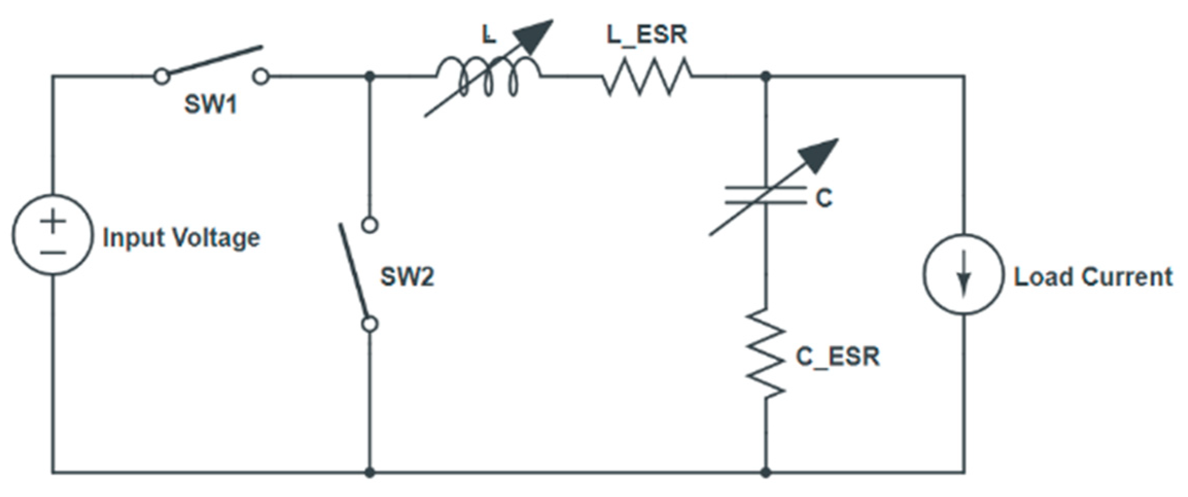
2.1. Buck Converter Parameters

Figure 1 displays the DC-DC buck converter model used in the simulation and experimentation of this work, and

Table 1. Buck converter circuit parameters.

Buck Converter Circuit Parameters
Inductance	$110 \mathrm{u}\mathrm{H},220 \mathrm{u}\mathrm{H}$
Capacitance	$150 \mathrm{u}\mathrm{F},300 \mathrm{u}\mathrm{F},450 \mathrm{u}\mathrm{F},600 \mathrm{u}\mathrm{F}$
Switch Resistance	$1 \mathrm{m}\mathrm{\Omega }$
Capacitive ESR	$120 \mathrm{m}\mathrm{\Omega }$
Inductive ESR	$7 \mathrm{m}\mathrm{\Omega }$

lists the converter’s parameters. It should be noted that the inductor and capacitor values vary, so multiple values are listed.

Combinations of inductor and capacitor values result in various configurations of the buck converter. The configurations are listed in

Table 2. Buck converter configurations.

Buck Converter Configurations
Configuration 1	Capacitance: $150 \mathrm{u}\mathrm{F}$	Inductance: $110 \mathrm{u}\mathrm{H}$
Configuration 2	Capacitance: $300 \mathrm{u}\mathrm{F}$	Inductance: $110 \mathrm{u}\mathrm{H}$
Configuration 3	Capacitance: $450 \mathrm{u}\mathrm{F}$	Inductance: $110 \mathrm{u}\mathrm{H}$
Configuration 4	Capacitance: $600 \mathrm{u}\mathrm{F}$	Inductance: $110 \mathrm{u}\mathrm{H}$
Configuration 5	Capacitance: $150 \mathrm{u}\mathrm{F}$	Inductance: $220 \mathrm{u}\mathrm{H}$
Configuration 6	Capacitance: $300 \mathrm{u}\mathrm{F}$	Inductance: $220 \mathrm{u}\mathrm{H}$
Configuration 7	Capacitance: $450 \mathrm{u}\mathrm{F}$	Inductance: $220 \mathrm{u}\mathrm{H}$
Configuration 8	Capacitance: $600 \mathrm{u}\mathrm{F}$	Inductance: $220 \mathrm{u}\mathrm{H}$

.

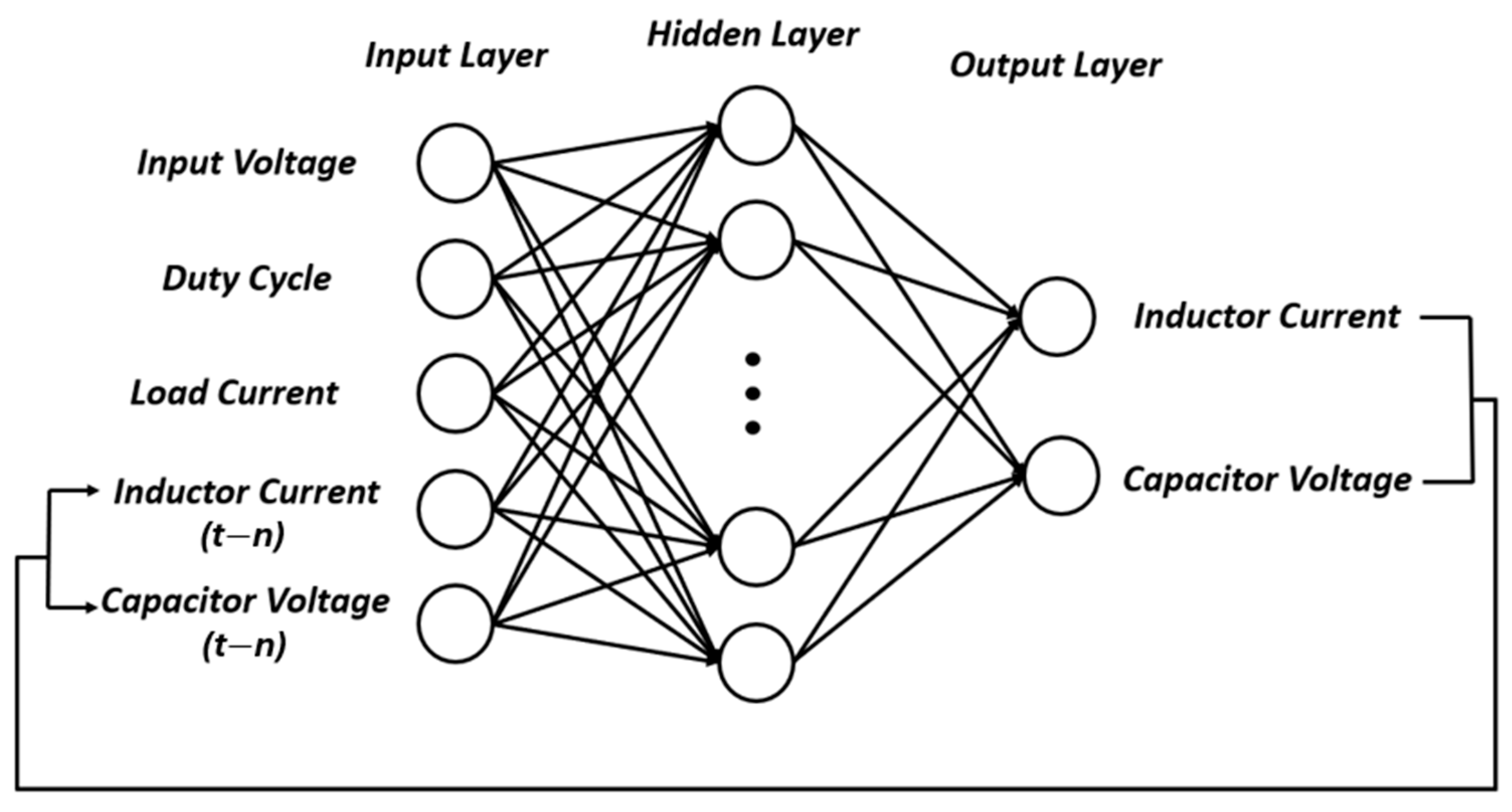
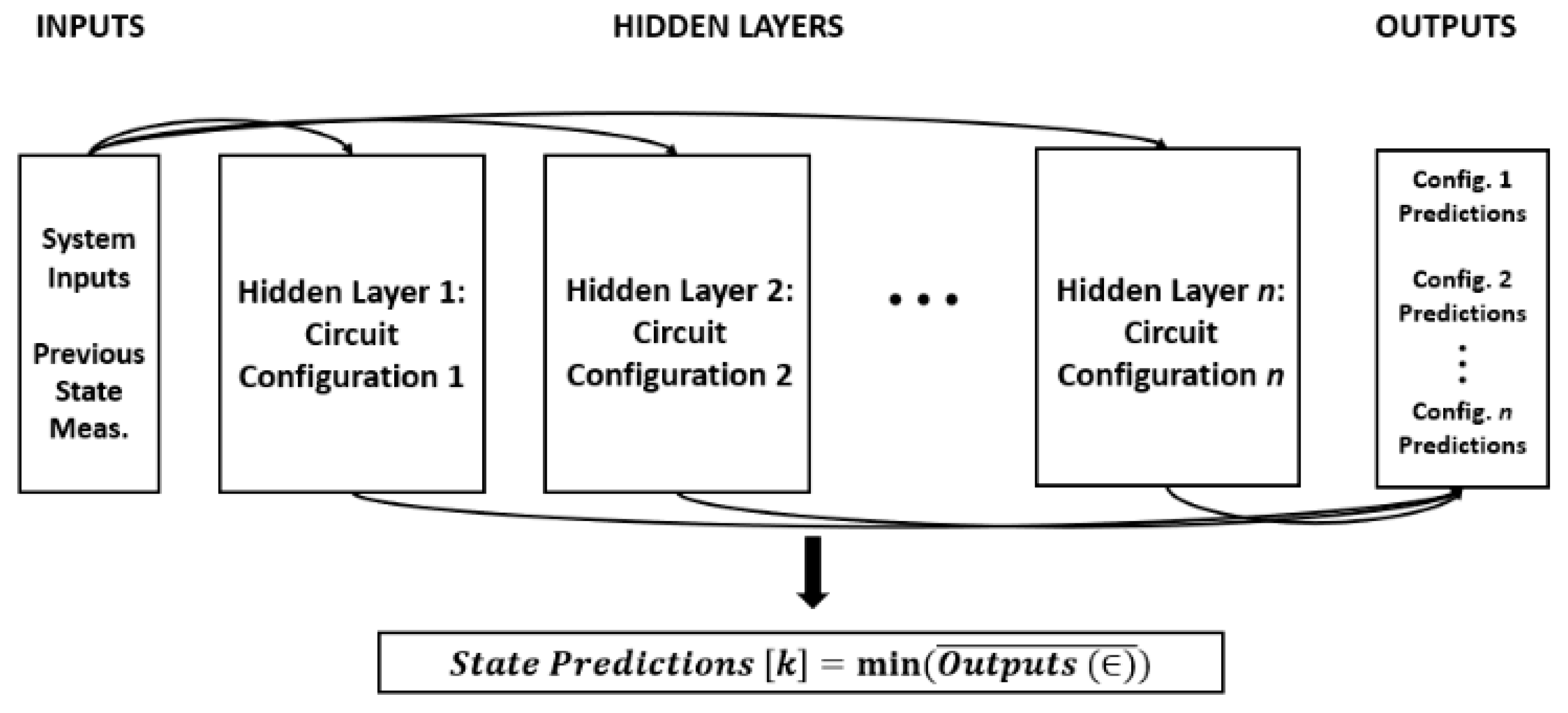
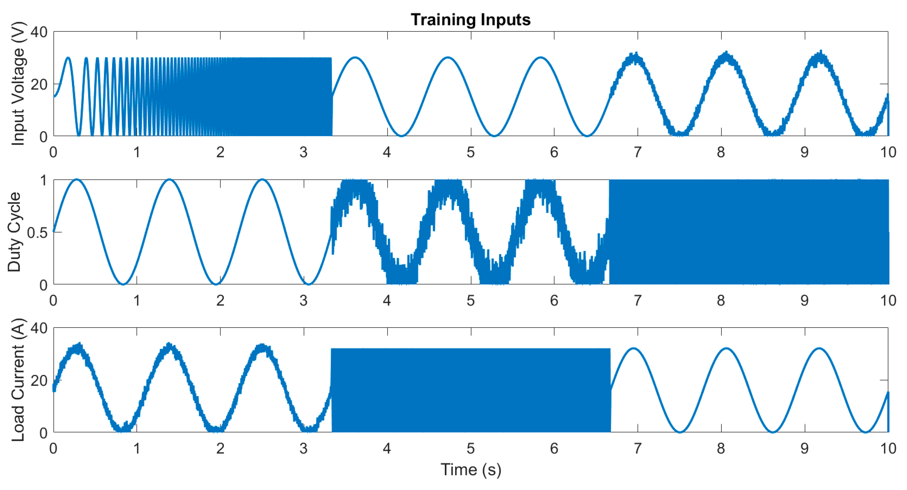
2.2. Modular Digital Twin Development

A recurrent neural network (RNN) is a type of artificial neural network that learns time-related dependencies in sequential data. An RNN can be developed to predict instantaneous buck converter states based on real-time input voltage, duty cycle, load current, and previous state estimation values. For this work, a NARX-RNN model was developed in MATLAB version R2022a. This model, as depicted in Figure 2, estimates instantaneous states of the buck converter, $\widehat{y}\left(k\right)$, based on input values, $u\left(k\right)$, and previous estimated state values, $\widehat{y}(k-n)$, where $k$ is the current time step and $n$ is measurement feedback delay. A mathematical representation of the NARX with closed loop feedback is presented as follows:

$$\widehat{y}\left(k\right)=F\left[\widehat{y}\left(k-1\right),\dots ,\widehat{y}\left(k-n\right),u\left(k-1\right),\dots , u\left(k-n\right)\right],$$

where $F$ represents the nonlinear function modeled by the network.

Unlike traditional RNN or Long-Short Term Memory (LSTM) networks, NARX-RNNs do not have internal feedback connections. Nodes within the model’s hidden layers, as seen in Figure 3, operate similarly to a feed-forward model. Each node processes input information and can be represented as follows:

$$Output=Wx+b,$$

where $W$ and $b$ are the weight and bias of the node, respectively, and $x$ is input information. The output of the node is then passed to an activation function, which is the source of the model’s nonlinearity.

The external feedback allows for them to learn temporal dependencies within data without the need for additional internal connections. This makes them less computationally expensive than their traditional counterparts, while still being able to learn time-specific system dynamics.

Each parameter configuration of the buck converter is trained using separate NARX-RNN models. All individual networks comprise five inputs, (input voltage, duty cycle, and load current, and past estimated states), two outputs (inductor current and capacitor voltage), one hidden layer with fifteen nodes, and a two-timestep feedback (measurement) delay. This model construction is presented in [27], and was shown to provide accurate state estimations for a DC-DC converter.

One potential modification that can be applied to NARX-RNNs is the removal of the feedback connection during network implementation. By removing the feedback connection, which would only allow for an averaged state prediction, the network has the ability to utilize previous system measurements, $y(k-n)$, rather than previous network state predictions, $\widehat{y}(k-n)$. This changes the mathematical representation to

$$\widehat{y}\left(k\right)=F\left[y\left(k-1\right),\dots ,y\left(k-n\right),u\left(k-1\right),\dots , u\left(k-n\right)\right].$$

In this section, it will be shown that this leads to increased prediction abilities, such as capturing system ripples, and increased prediction robustness and adaptability as system parameters experience small variations.

The construction of the NARX-RNN models representing each converter configuration is consistent, but variations exist within the weights and biases of the hidden layers. Because of this, one set of system inputs (input voltage, duty cycle, and load current) can be used to predict system states for each buck converter configuration simultaneously. Skipped layer connections, which are neural network connections that bypass intermediate layers, would allow for individual networks to be combined into a larger, modular, NARX-RNN model. An example of a combined model is shown in Figure 4. The hidden layers, which represent different variations of the converter, receive the converter’s inputs via the skipped layer connections. Each hidden-layer model representation then produces its own state estimation outputs. This provides a digital twin model that produces multiple potential state estimations for a variety of the buck converter’s parameter combinations. The state estimations that are most accurate relative to the converter’s parameters have the lowest mean estimation error, $\mathrm{m}\mathrm{i}\mathrm{n}\left(\overline{Outputs(\in )}\right)$, where $\in$ is the absolute error between the measured and predicted state; these are selected for circuit monitoring.

This adaptation of a traditional NARX-RNN model allows for a single digital twin to model various buck converters without the need for new model development or retraining after implementation. For parameter variations that exist outside of the pretrained models’ prediction capabilities, additional parameter-specific hidden layers and skipped connections can be added to the existing model. This modularity allows for the digital twin to remain adaptable to the constantly changing circuit parameters and operating environments the converters are exposed to in maritime microgrid applications.

The development of the individual networks begins with collecting training data from the Simulink buck converter described in Section 2. A combination of a sine wave, a sine wave with Gaussian white noise, and a chirp signal were simultaneously applied to the input voltage, duty cycle, and load current of the converter. The varying system inputs can be seen in Figure 5. The resulting inductor current and capacitor voltage can be seen in Figure 6 and Figure 7, respectively. This method of input variation is presented in [26], and allows the NARX-RNN models to be exposed to a wide variety of system operating points. It should be noted that this buck converter model was configured with two switches, as it would be in a bidirectional DC-DC converter. Because of this, no diode was present to oppose the flow of negative current, and this occasionally resulted in a non-positive inductor current and capacitor voltage. For experimental testing, a diode was added to ensure the converter was not exposed to negative inductor current or output voltage.

Once the training data was collected for each buck converter configuration, it was used to train multiple configuration-specific NARX-RNN models. As previously mentioned, the individual NARX-RNN models comprised five inputs, (input voltage, duty cycle, and load current, and past estimated states), two outputs (inductor current and capacitor voltage), one hidden layer with fifteen nodes, and a two-timestep feedback (measurement) delay. Each model was trained with the Levenberg–Marquardt training algorithm, and the data was randomly divided, with 70% being used for training, 15% being used for validation, and the remaining 15% being used for testing.

3. Simulation Results

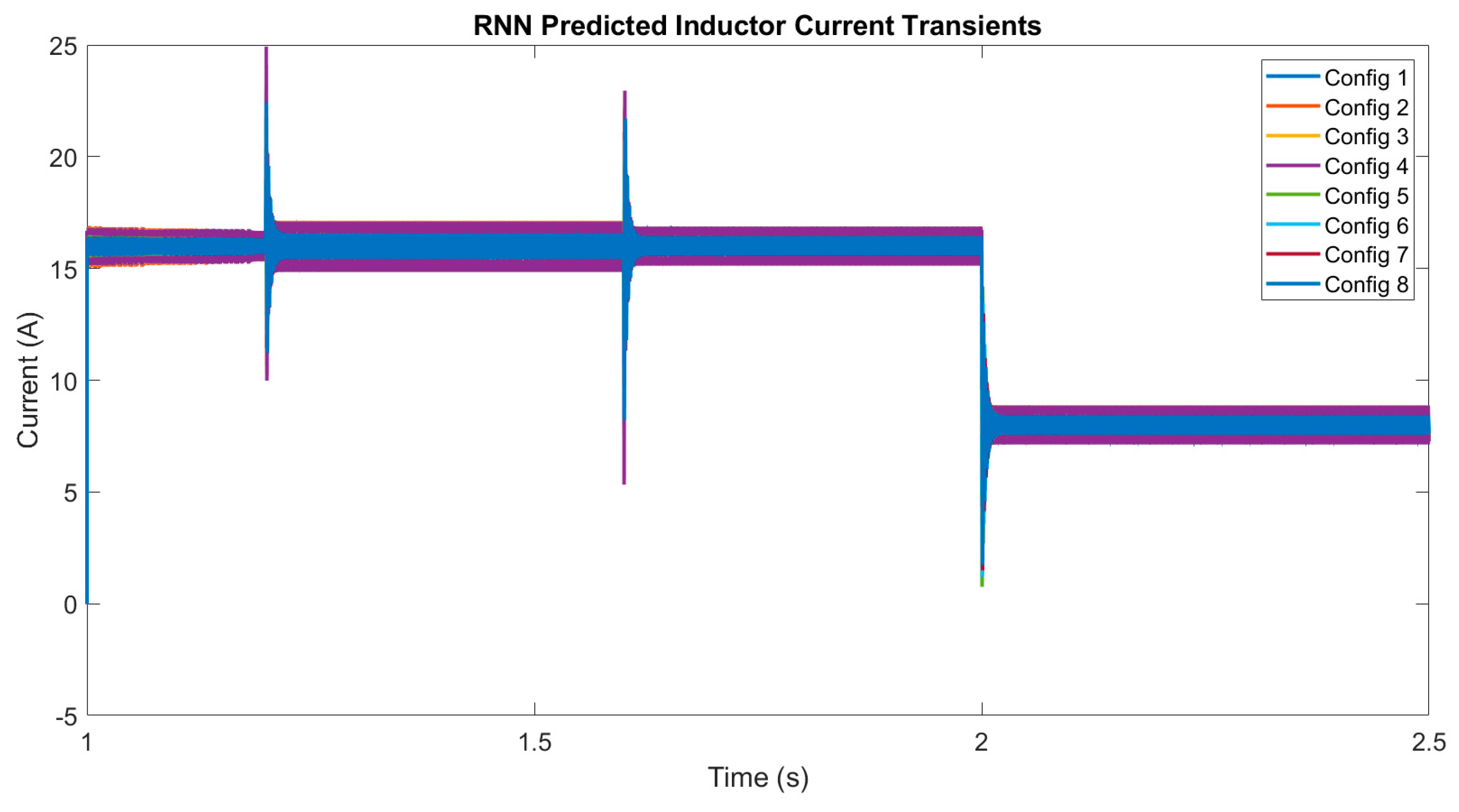
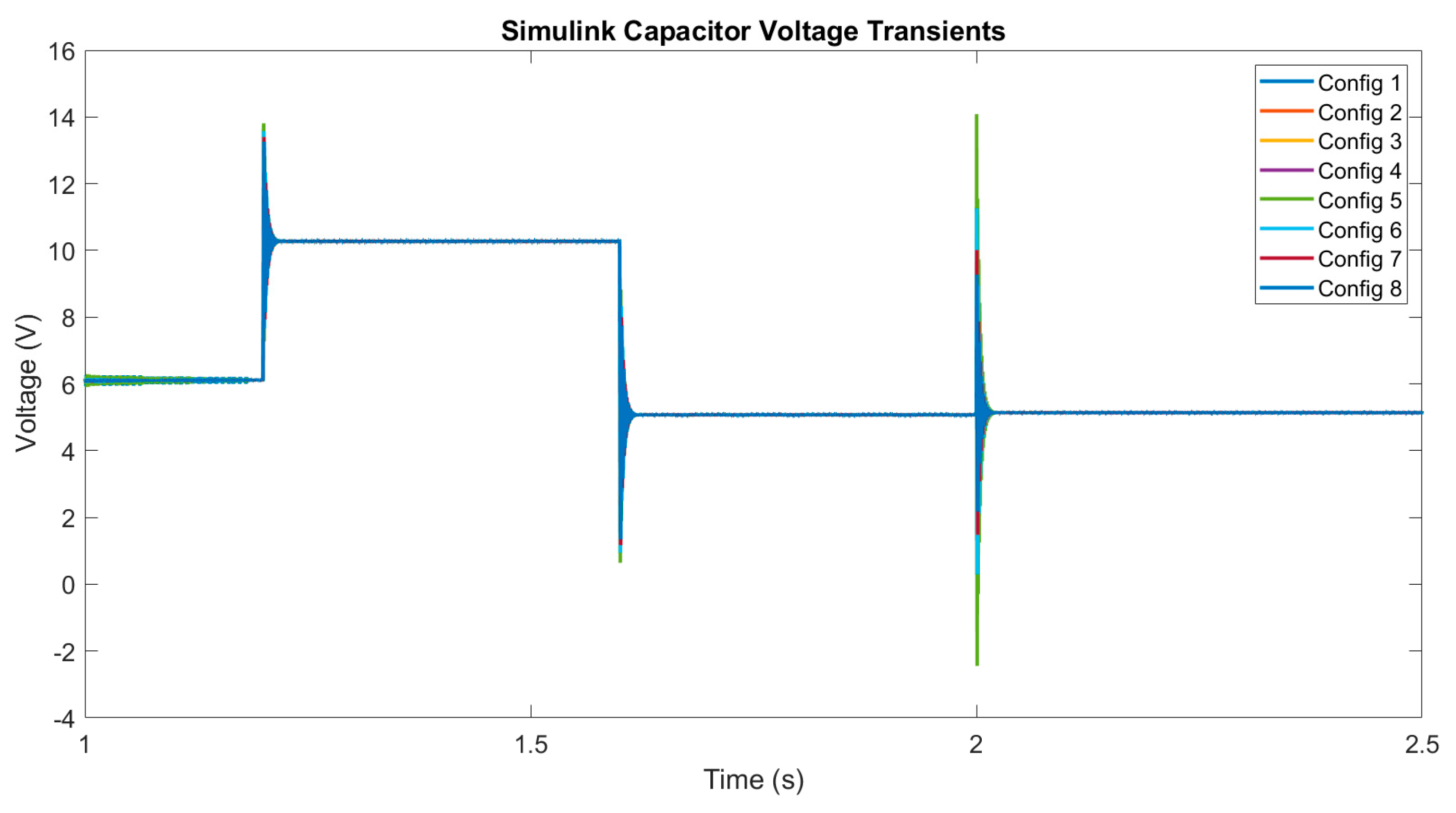
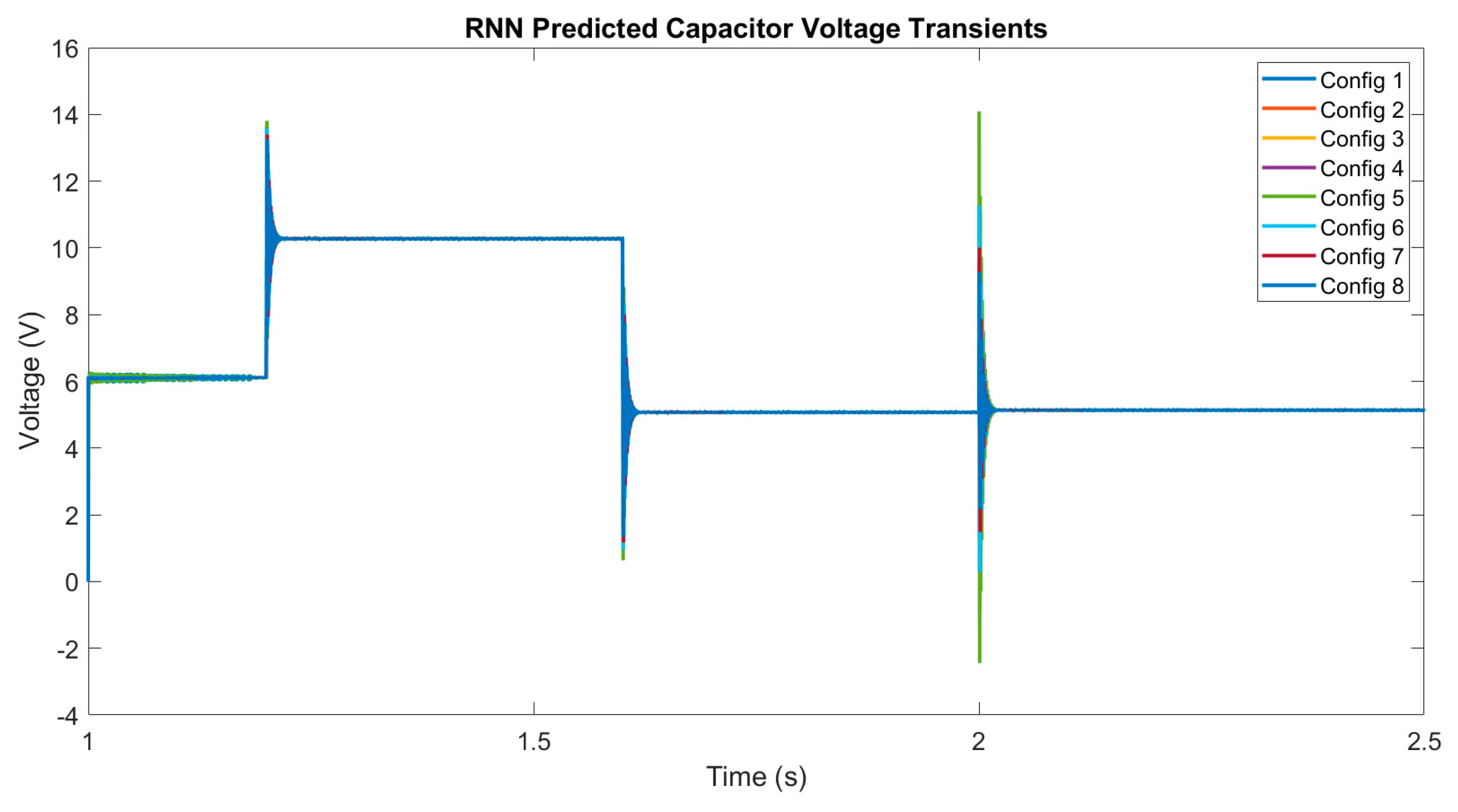
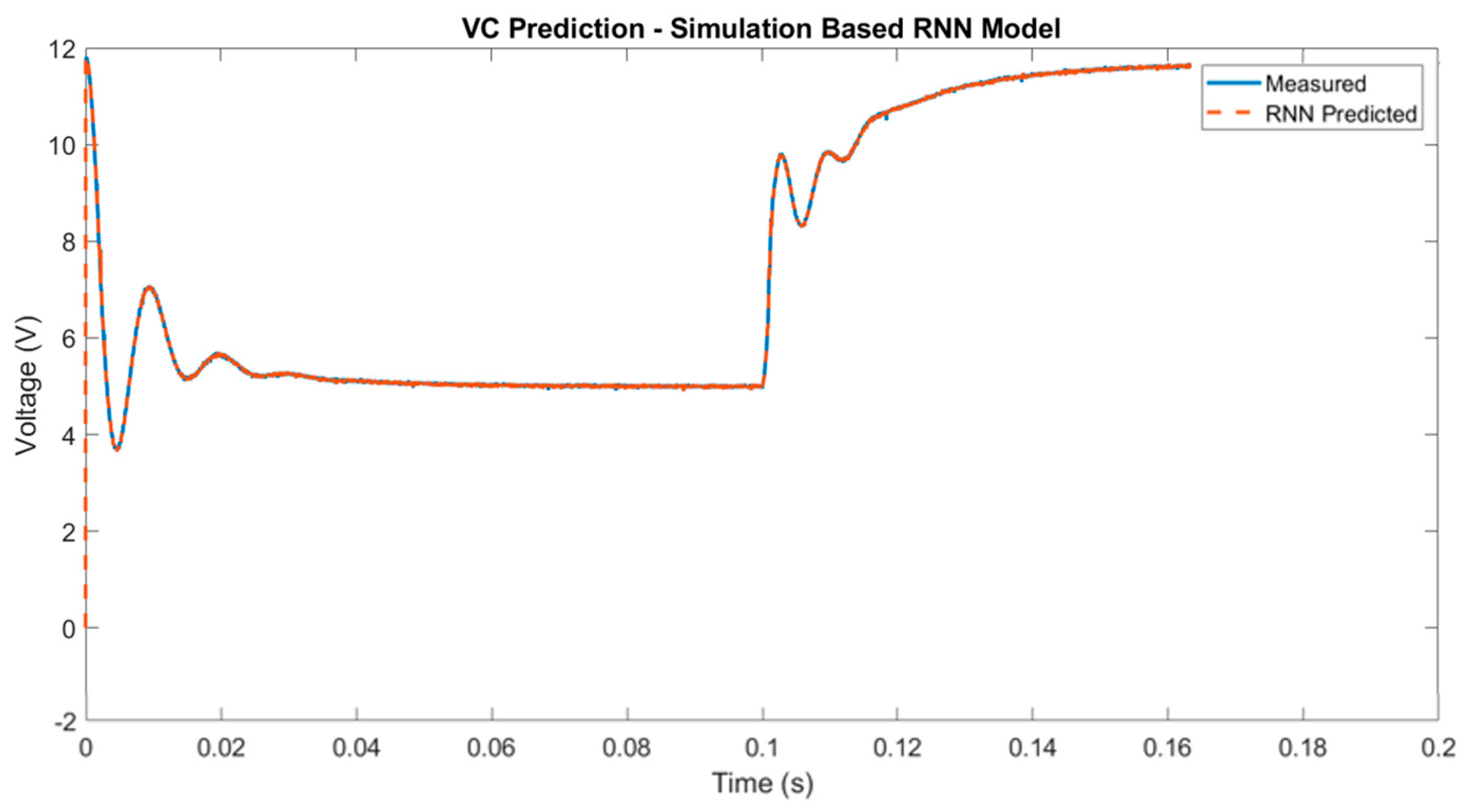
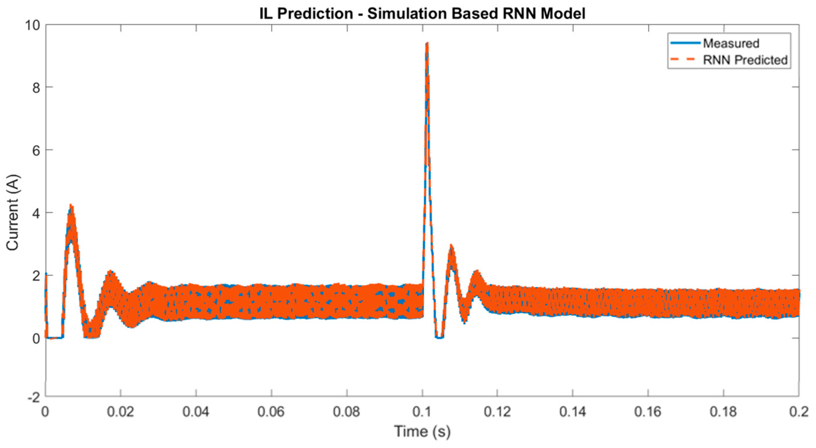
3.1. Digital Twin Testing for Model Trained with Simulated Data

After training was completed for each buck converter variation, the individual NARX-RNN models were combined into the modular NARX-RNN model, which consisted of five system inputs and eight hidden layers. The modular model’s state prediction and model identification accuracy were tested by evaluating its state estimation ability as a result of step changes in system inputs and previous state measurements for each converter configuration. Figure 8 displays the input step changes applied to the simulations and NARX-RNN models. Figure 9, Figure 10, Figure 11 and Figure 12 show comparisons between the Simulink and NARX-RNN state predictions for all eight buck converter configurations. It can be seen from the images that each converter configuration-specific NARX-RNN model layer closely follows the transient of its corresponding Simulink model. Additionally, it can be seen that the modular NARX-RNN model has the ability to make state estimations for various buck converter configurations.

As the network makes state predictions, the hidden layer that results in the lowest average estimation error is utilized for future predictions. For this work, the mean of the error is calculated over the entire 2.5 s testing interval, but this duration can be modified based on system-specific requirements. To demonstrate how the error rate of each layer changes relative to the various configurations of the buck converter,

Table 3. Mean inductor current prediction error.

Inductor Current RNN Prediction Error Mean
	Layer 1	Layer 2	Layer 3	Layer 4	Layer 5	Layer 6	Layer 7	Layer 8		Scale
Config 1	0.1416	0.1608	0.1626	0.1627	0.2674	0.2707	0.2740	0.2761		0.0703
Config 2	0.1613	0.1407	0.1591	0.1618	0.2520	0.2709	0.2744	0.2766		0.0998
Config 3	0.1625	0.1584	0.1414	0.1553	0.2675	0.2656	0.2735	0.2765		0.1293
Config 4	0.1638	0.1623	0.1566	0.1401	0.2705	0.2536	0.2703	0.2758		0.1587
Config 5	0.2649	0.2508	0.2647	0.2682	0.0709	0.1012	0.1044	0.1070		0.1882
Config 6	0.2681	0.2697	0.2628	0.2512	0.1013	0.0708	0.1022	0.1074		0.2177
Config 7	0.2714	0.2731	0.2707	0.2679	0.1049	0.1027	0.0703	0.1008		0.2471
Config 8	0.2735	0.2753	0.2737	0.2735	0.1071	0.1074	0.1005	0.0707		0.2766

and

Table 4. Mean capacitor voltage prediction error.

Capacitor Voltage RNN Prediction Error Mean
	Layer 1	Layer 2	Layer 3	Layer 4	Layer 5	Layer 6	Layer 7	Layer 8		Scale
Config 1	0.0004	0.0133	0.0125	0.0127	0.0173	0.0156	0.0155	0.0160		0.0003
Config 2	0.0333	0.0023	0.0176	0.0210	0.0211	0.0334	0.0345	0.0349		0.0073
Config 3	0.0355	0.0182	0.0022	0.0110	0.0359	0.0231	0.0276	0.0283		0.0143
Config 4	0.0371	0.0218	0.0116	0.0011	0.0395	0.0160	0.0226	0.0250		0.0213
Config 5	0.0494	0.0215	0.0351	0.0385	0.0020	0.0430	0.0450	0.0461		0.0283
Config 6	0.0484	0.0341	0.0237	0.0165	0.0439	0.0006	0.0310	0.0333		0.0354
Config 7	0.0486	0.0352	0.0280	0.0231	0.0458	0.0313	0.0003	0.0235		0.0424
Config 8	0.0491	0.0355	0.0288	0.0254	0.0469	0.0336	0.0237	0.0005		0.0494

show the mean of the state prediction error for the inductor current and capacitor voltage, respectively, over the testing interval. Heatmaps were applied to the tables, and the corresponding scales are located to the right of the tables. In the scales, lower error means are represented with shades of green and larger values are represented with shades of red. In each table, the hidden layer corresponding to its correct buck converter configuration has the lowest error mean for inductor current and capacitor voltage. This can be most clearly seen by observing that the mean error values in the main diagonal of each table provide the lowest mean error of all converter configurations within each respective column.

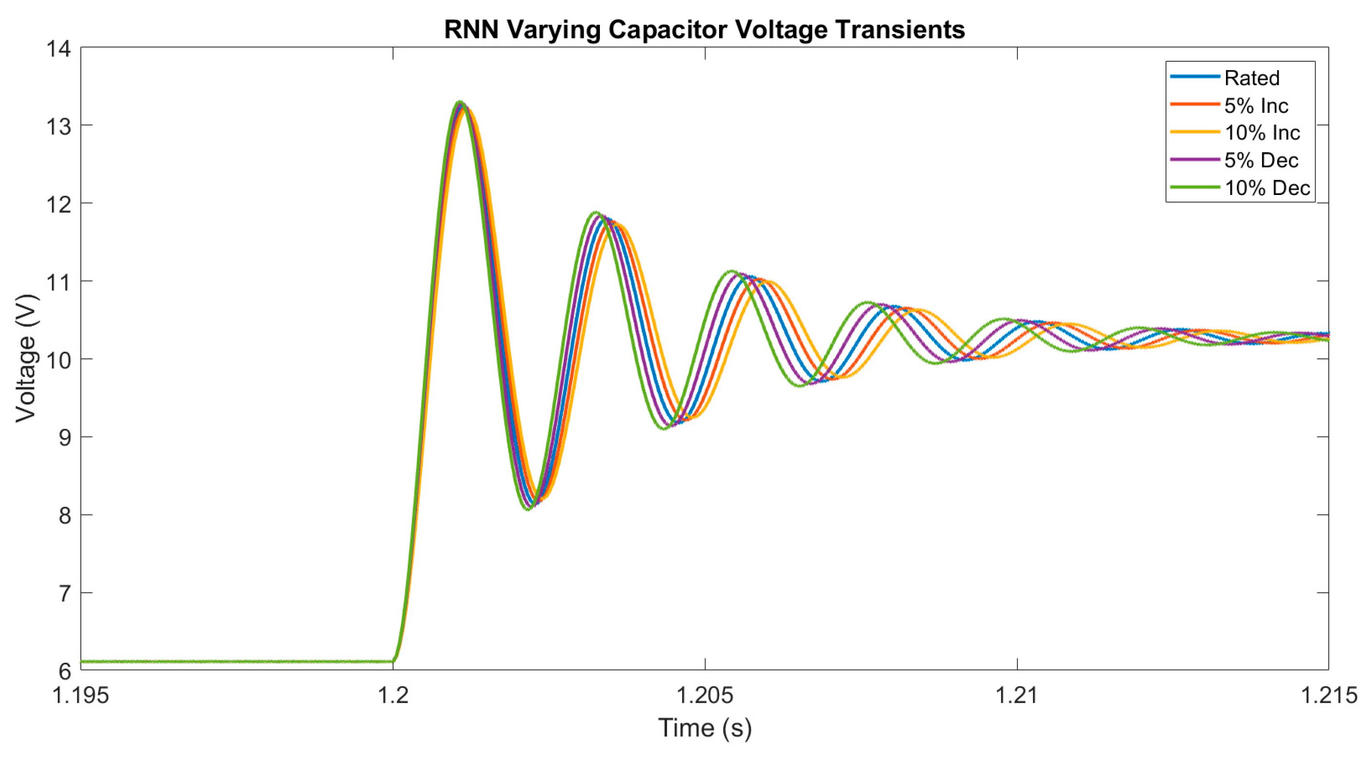
3.2. Model Prediction Accuracy for Small Component Variations

Next, the prediction accuracy of the modular NARX-RNN model is tested against the measured states from the buck converter with small variations in the inductor and capacitor values. In practical applications, inductors and capacitors have tolerances relative to their nominal values. These tolerances indicate that the nominal values of the components exist within a percentage of their rated values. Additionally, factors such as component aging and operating environments can cause fluctuations in the component’s values. In a NARX-RNN model with a closed feedback loop, small parameter fluctuations would lead to increased prediction errors due to their isolation from measurement data. However, when the model uses previous system measurements rather than previously predicted states, the robustness of the NARX-RNN is increased, and prediction accuracy is maintained for small component variations.

To demonstrate this, layer 8 of the modular NARX-RNN was used to test the prediction accuracy of configuration 8 of the buck converter Simulink model, with 5 and 10 percent variations in the inductor and capacitor. For this test, the buck converter components were isolated and varied by increasing and decreasing their rated values by 5 and 10 percent. When including the rated value, this allows for five potential component variations within 10 percent of the rated value for both components. The testing inputs from Figure 7 were applied to the configuration 8 Simulink model with five variations in the inductor and capacitor. The resulting measurement data from each of the 10 simulations was collected and used for testing layer 8 of the centralized model, which was not altered. Layer 8 received inputs from Figure 8 and feedback data from each of the 10 simulations. Figure 13 and Figure 14 show the predictions of the inductor current and capacitor voltage, respectively, as a result of the collected Simulink data. From the images, it can be seen that the unaltered layer 8 of the centralized NARX-RNN model was able to predict differing transient responses for each component variation. In

Table 5. Prediction error for small component variations.

RNN Prediction Error for Small Component Variations
	Rated	5% Increase	10% Increase	5% Decrease	10% Decrease
IL Error Mean (A)	0.0707	0.0673	0.0642	0.0744	0.0786
IL Error Variance (A)	0.0014	0.0013	0.0013	0.0016	0.0017
VC Error Mean (V)	5.04 × 10−4	5.09 × 10−4	5.18 × 10−4	5.04 × 10−4	5.11 × 10−4
VC Error Variance (V)	4.99 × 10−5	4.99 × 10−5	4.99 × 10−5	4.99 × 10−5	4.99 × 10−5

, the mean and variance of the absolute prediction errors are shown for each component variation. The state prediction error rates remained relatively consistent even as the component values varied in the simulation. This confirms the network’s ability to make consistently accurate predictions even in the presence of small parameter variation, thus reducing the need for intermittent retraining.

4. Experimental Results

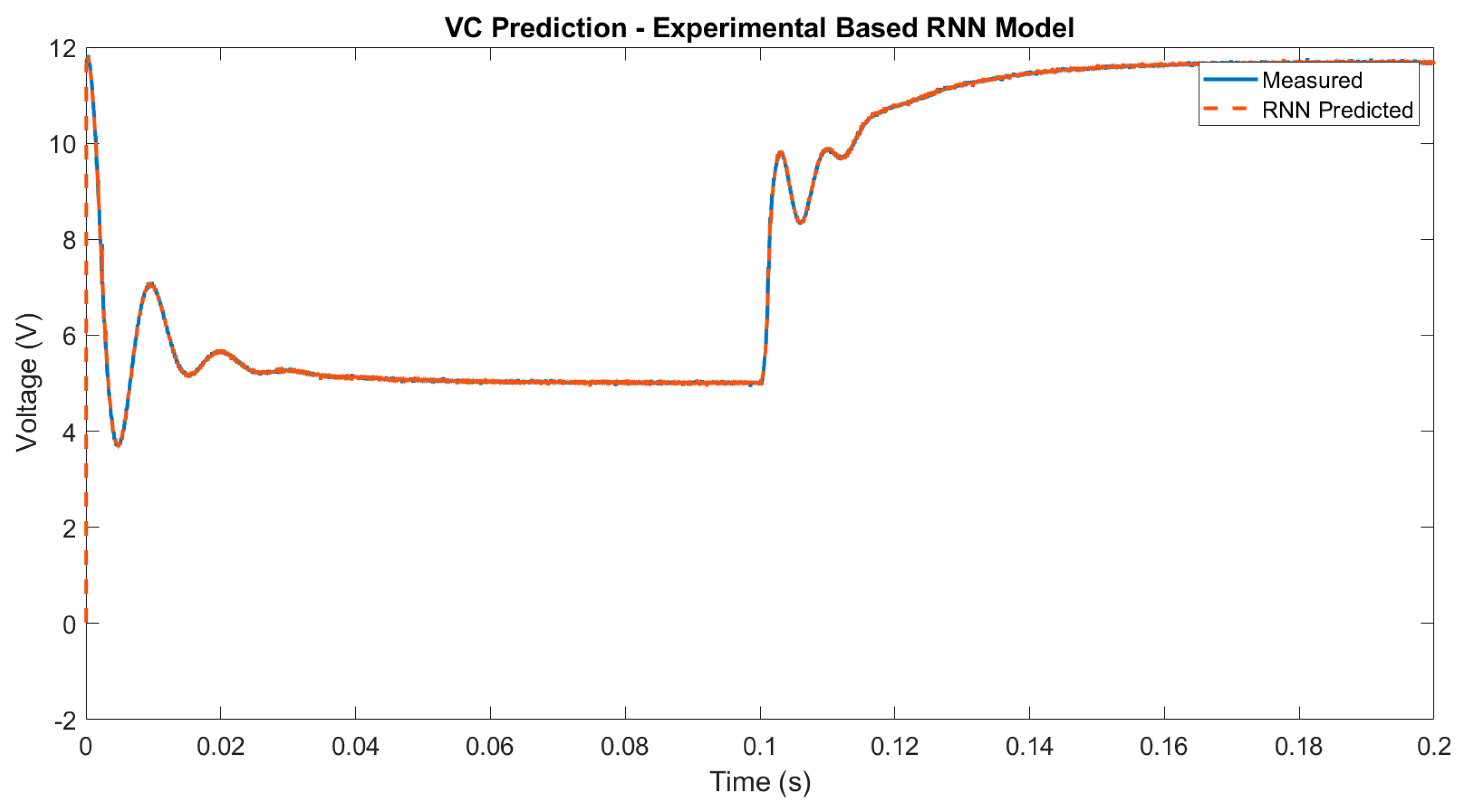
4.1. Digital Twin Testing for Model Trained with Experimental Data

The experimental validation of the variable configuration digital twin model was investigated using the buck converter shown in Figure 15. This converter was designed for variable circuit configurations through the integration of connectors that allow for the addition and removal of inductance and capacitance. The inductor and capacitor values are listed in Table 1, and the possible converter configurations are listed in Table 2, as demonstrated in the simulation. The system’s embedded controller utilized STM32CubeIDE software and an STM32G474RET6 microcontroller was used to execute testing algorithms. All measured circuit data was captured on a secure digital card and later processed in the MATLAB environment.

The digital twin development began by collecting state-variable data as a result of varying circuit inputs. In the simulation, inductor current and capacitor voltage were measured as system states. In the experiment, it was not possible to measure capacitor voltage independently of the additional voltage caused by the capacitive equivalent series resistance (ESR). Because of this, inductor current and capacitor voltage, including the capacitive ESR (output voltage), are represented as system states. The input voltage remained constant at 18 V and the duty cycle was varied from 0.1 to 0.9 in steps of 0.1, as seen in Figure 16, for multiple load currents between 0 A and 2 A. Using a similar approach to that used in the simulations, a separate NARX-RNN was trained for each buck converter configuration. The networks remained identical, consisting of an input layer with five inputs, one hidden layer with fifteen nodes, an output layer with the potential for feedback connection, and a two-timestep delay for feedback or previously measured system states. The networks were trained with the Levenberg–Marquardt training algorithm, and the training data was split up into 70%, 15%, and 15% for training, validation and testing, respectively.

After training was concluded for each model, testing was conducted for each converter configuration by applying an 18 V input and stepping the duty cycle from 0.35 to 0.75 for load current values of 0.5 and 1.5 A. The resulting measured and predicted output voltages for all buck converter configurations can be seen in Figure 17, Figure 18, Figure 19 and Figure 20. The measured and predicted output voltage values for both load current values demonstrate similar transient behaviors, and this is confirmed in error

Table 6. Mean capacitor voltage prediction error—0.5 A load current.

Capacitor Voltage RNN Prediction Error Mean—0.5A Load Current
	Layer 1	Layer 2	Layer 3	Layer 4	Layer 5	Layer 6	Layer 7	Layer 8		Scale
Config 1	0.0309	0.1148	0.1819	0.2490	0.2076	0.2098	0.2407	0.2781		0.0228
Config 2	0.1138	0.0279	0.0899	0.1606	0.2079	0.1508	0.1657	0.2009		0.0593
Config 3	0.1930	0.1113	0.0256	0.0767	0.2313	0.1177	0.1123	0.1503		0.0957
Config 4	0.2545	0.1753	0.0932	0.0279	0.2580	0.1292	0.0966	0.1176		0.1322
Config 5	0.1835	0.1841	0.2259	0.2598	0.0348	0.1793	0.2336	0.2411		0.1687
Config 6	0.2035	0.1482	0.1195	0.1325	0.1693	0.0234	0.1202	0.1817		0.2052
Config 7	0.2373	0.1708	0.1178	0.0903	0.2268	0.1163	0.0246	0.1282		0.2417
Config 8	0.2747	0.2041	0.1556	0.1201	0.2338	0.1831	0.1332	0.0228		0.2781

and

Table 7. Mean capacitor voltage prediction error—1.5 A load current.

Capacitor Voltage RNN Prediction Error Mean—1.5A Load Current
	Layer 1	Layer 2	Layer 3	Layer 4	Layer 5	Layer 6	Layer 7	Layer 8		Scale
Config 1	0.0316	0.1937	0.3030	0.3732	0.2197	0.2502	0.3298	0.4336		0.0250
Config 2	0.2085	0.0334	0.1844	0.2638	0.1772	0.1783	0.2253	0.3381		0.0839
Config 3	0.3037	0.1898	0.0295	0.1234	0.2697	0.1646	0.1446	0.2159		0.1427
Config 4	0.3768	0.2608	0.1407	0.0317	0.3649	0.2407	0.1656	0.1596		0.2016
Config 5	0.2093	0.1796	0.2646	0.3615	0.0369	0.2200	0.3242	0.4350		0.2605
Config 6	0.2523	0.1733	0.1632	0.2317	0.2187	0.0253	0.1693	0.3074		0.3193
Config 7	0.3372	0.2251	0.1500	0.1655	0.3164	0.1737	0.0268	0.1785		0.3782
Config 8	0.4371	0.3431	0.2225	0.1540	0.4330	0.3089	0.1767	0.0250		0.4371

, where the main diagonal displays the mean prediction error of each layer relative to its corresponding buck converter configuration. Similarly to the digital twin model for the simulated converter, the lowest prediction error occurred along the main diagonals of each table, demonstrating the model’s ability to differentiate converter configuration during output voltage prediction.

For inductor current, however, model predictions were not as accurate. During the simulation, the training data inputs consisted of simultaneously changing sinusoids, as shown in Figure 5. This allowed for a wide variety of continuous system transients. Experimental training data, however, was limited by the DC power and load sources’ inability to continually change. Rather than a combination of sinusoids, this data consisted of step changes in duty cycle at various load current values while input voltage remained constant. This resulted in considerably fewer transient dynamics, and, as a result, less diversity was present in the training data. Additionally, a diode existed in the experimental buck converter that did not allow for negative inductor current, further limiting the diversity of the data. This resulted in the circuit operating in discontinuous conduction mode for low load current values, leading to inconsistencies in inductor current dynamics as the load current varied. The comparatively limited transient data variation and inconsistent dynamics in network inductor current training data led to poor transient prediction accuracy in the modular digital twin model. This is demonstrated in Figure 21, Figure 22, Figure 23 and Figure 24, where it can be seen that the measured transient responses remain positive but the digital twin makes nonpositive predictions. The prediction error of the buck converter configurations relative to the centralized model layers is presented in

Table 8. Mean inductor current prediction error—0.5 A load current.

Inductor Current RNN Prediction Error Mean—0.5A Load Current
	Layer 1	Layer 2	Layer 3	Layer 4	Layer 5	Layer 6	Layer 7	Layer 8		Scale
Config 1	0.2605	0.2228	0.2701	0.5116	0.5793	0.5877	0.5743	0.5772		0.1257
Config 2	0.3250	0.2235	0.2305	0.4921	0.6243	0.5973	0.5930	0.5973		0.2077
Config 3	0.5308	0.4658	0.2305	0.3081	0.6997	0.5335	0.4439	0.5290		0.2897
Config 4	0.6721	0.6125	0.4524	0.2190	0.6149	0.3393	0.3842	0.3208		0.3717
Config 5	0.4604	0.4215	0.5649	0.5960	0.2771	0.4200	0.6366	0.4245		0.4537
Config 6	0.6662	0.6180	0.6113	0.4622	0.4149	0.2245	0.5468	0.2644		0.5357
Config 7	0.6293	0.5953	0.4810	0.2736	0.5524	0.3129	0.3087	0.2651		0.6177
Config 8	0.6150	0.5899	0.5874	0.4330	0.3856	0.1928	0.5035	0.1257		0.6997

and

Table 9. Mean inductor current prediction error—1.5 A load current.

Inductor Current RNN Prediction Error Mean—1.5A Load Current
	Layer 1	Layer 2	Layer 3	Layer 4	Layer 5	Layer 6	Layer 7	Layer 8		Scale
Config 1	0.2908	0.5997	0.7520	0.5065	0.7123	0.4781	0.4772	0.6017		0.1555
Config 2	0.8210	0.3078	0.9155	0.8467	0.7438	0.7230	0.6435	0.7523		0.2641
Config 3	0.6146	0.8839	0.2992	0.3593	0.6206	0.4176	0.7600	0.4952		0.3727
Config 4	0.2801	0.6791	0.5723	0.2902	0.6476	0.3411	0.5656	0.5035		0.4812
Config 5	0.6528	0.7037	0.3110	0.4969	0.3769	0.4333	0.6443	0.4527		0.5898
Config 6	0.4639	0.6085	0.5577	0.4455	0.5974	0.2700	0.4179	0.4664		0.6984
Config 7	0.6491	0.4056	0.7517	0.6591	0.6612	0.4838	0.3291	0.5268		0.8069
Config 8	0.4719	0.6925	0.4301	0.3470	0.4624	0.2651	0.5346	0.1555		0.9155

for 0.5 A and 1.5 A load currents, respectively. For a load current of 0.5 A, model identification was not as accurate as that of output voltage, with layers 1 and 7 not demonstrating the lowest average prediction error for their respective converter configuration. For a load current of 1.5 A, layers 4 and 5 exhibited similar behavior. Various network configurations with an increased number of hidden layers and layer nodes were tested, and various training methods were attempted, but prediction accuracy remained consistent across all variations. Without the ability to provide greater variation in the input training data, model generalization is limited, and model implementation will result in poor inductor current estimation.

4.2. Digital Twin Trained with Experimental Data Tested on a Physical Converter

The lack of accurate experimental transient training data resulted in poor inductor current state predictions during transient events. In Section 3, the digital twin developed with simulated training data was exposed to a larger variety of system transients. This led to more accurate state predictions than the physical data-trained digital twin, even in the presence of small component variations. Data-driven systems rely on empirical system data for training, so the application of a NARX model developed with simulated measurements does not align with standard practices. However, the simulation-based model’s demonstrated adaptability to parameter variation encourages the theory than it can be applied to physical systems even without being trained with physical data. Because of this, the digital twin developed with simulation training data was tested on the physical buck converter to demonstrate the applicability of a model developed with simulated data in a physical system.

Converter configuration 8 provided the most accurate experimental inductor current predictions due to the converter remaining in continuous conduction mode. Because of this, hidden layer 8 of the centralized digital twin models developed with simulated and physical data was used for comparison. Layer 8 of both digital twins was tested with an 18 V input and the duty cycle was increased from 0.35 to 0.75 with a load current of 1.5 A. Previously measured physical system states were used as feedback inputs for both digital twin models. Figure 25, Figure 26, Figure 27 and Figure 28 and

Table 10. Mean state prediction error for simulation-based digital twin applied to physical buck converter.

Mean State Prediction Error for Simulation-Based Digital Twin Applied to Physical Buck Converter
	0.5 A Load Current	1.5 A Load Current
Inductor Current	0.0733 A	0.0725 A
Capacitor Voltage	0.0211 V	0.0319 V

provide a comparison of measured and predicted buck converter states. It can be seen that output voltage prediction accuracy is similar, regardless of whether the model is trained with simulated or experimental data. Although the simulated data provides more transient system behaviors during training, the experimental training data was able to capture enough system dynamics to properly model capacitor voltage. The inductor current prediction accuracy, however, is considerably better when using the model developed with simulated training data. This demonstrates the simulation-based digital twin’s ability to accurately predict the system states of physical converters even when only trained using simulated data.

5. Conclusions

A centralized, modular digital twin was developed for a variable configuration buck converter. During simulation, the digital twin was able to accurately predict system states and correctly identify the converter configuration based on prediction accuracy, even in the presence of small parameter variations. During the experiment, the digital twin developed using experimental training data was able to accurately predict transient output voltage, but provided poor transient predictions for the inductor current. The twin developed with simulated training data, however, was able to make accurate output voltage, inductor current, and model identification predictions for the physical circuit used in the experiments. This demonstrated the single digital twin’s ability to model multiple circuit configurations and provided evidence that a model trained with simulated data can be integrated for use in physical circuit state prediction and configuration identification, challenging traditional data-driven model development methodologies.

Future work will further investigate the centralized model’s application to addition converter topologies and explore its integration into real-time embedded systems. Additionally, the model’s demonstrated ability to adapt to parameter variations encourages its use in fault detection, health monitoring, and adaptive control. These advancements have the potential to improve the monitoring, safety, and efficiency of power electronics within microgrids in maritime environments.

References

1. McCoy, T.J. Electric Ships Past, Present, and Future [Technology Leaders]. IEEE Electrif. Mag. 2015, 3, 4–11. [Google Scholar] [CrossRef]
2. Jin, Z.; Sulligoi, G.; Cuzner, R.; Meng, L.; Vasquez, J.C.; Guerrero, J.M. Next-Generation Shipboard DC Power System: Introduction Smart Grid and DC Microgrid Technologies into Maritime Electrical Networks. IEEE Electrif. Mag. 2016, 4, 45–57. [Google Scholar] [CrossRef]
3. Al-Falahi, M.D.A.; Tarasiuk, T.; Jayasinghe, S.G.; Jin, Z. AC ship microgrids: Control and power management optimization. Energies 2018, 11, 1458. [Google Scholar] [CrossRef]
4. Fang, S.; Wang, Y.; Gou, B.; Xu, Y. Toward Future Green Maritime Transportation: An Overview of Seaport Microgrids and All-Electric Ships. IEEE Trans. Veh. Technol. 2020, 69, 207–219. [Google Scholar] [CrossRef]
5. de la Cruz, J.; Wu, Y.; Candelo-Becerra, J.E.; Vásquez, J.C.; Guerrero, J.M. Review of Networked Microgrid Protection: Architectures, Challenges, Solutions, and Future Trends. CSEE J. Power Energy Syst. 2024, 10, 448–467. [Google Scholar]
6. Peyghami, S.; Fotuhi-Firuzabad, M.; Blaabjerg, F. Reliability Evaluation in Microgrids with Non-Exponential Failure Rates of Power Units. IEEE Syst. J. 2020, 14, 2861–2872. [Google Scholar] [CrossRef]
7. Peyghami, S.; Blaabjerg, F.; Fotuhi-Firuzabad, M. Model-Based Reliability-Centered Design of Power Electronics Dominated Microgrids. In Proceedings of the 2022 17th International Conference on Probabilistic Methods Applied to Power Systems (PMAPS), Manchester, UK, 12–15 June 2022; pp. 1–6. [Google Scholar]
8. Yang, S.; Bryant, A.; Mawby, P.; Xiang, D.; Ran, L.; Tavner, P. An Industry-Based Survey of Reliability in Power Electronic Converters. IEEE Trans. Ind. Appl. 2011, 47, 1441–1451. [Google Scholar] [CrossRef]
9. Ma, Z.; Li, Y.; Feng, J.; Fu, N.; Shi, W.; Liang, D. Influence of Power Electronic Devices Failure Rate on Wind Turbine System Reliability. In Proceedings of the 2024 8th International Conference on Green Energy and Applications (ICGEA), Singapore, 14–16 March 2024; pp. 192–195. [Google Scholar]
10. Peyghami, S.; Davari, P.; Fotuhi-Firuzabad, M.; Blaabjerg, F. Failure Mode, Effects and Criticality Analysis (FMECA) in Power Electronic-Based Power Systems. In Proceedings of the 2019 21st European Conference on Power Electronics and Applications (EPE ’19 ECCE Europe), Genova, Italy, 3–5 September 2019; pp. P.1–P.9. [Google Scholar]
11. Li, C.; Spro, O.C.; Fosso, O.B. Lifetime Modelling of Power Electronics for Power Electronic-Based Power System—A Case for Microgrids. In Proceedings of the 2021 IEEE/IAS Industrial and Commercial Power System Asia (I&CPS Asia), Chengdu, China, 18–21 July 2021; pp. 483–488. [Google Scholar]
12. Tao, F.; Zhang, H.; Liu, A.; Nee, A.Y.C. Digital Twin in Industry: State-of-the-Art. IEEE Trans. Ind. Inform. 2019, 15, 2405–2415. [Google Scholar] [CrossRef]
13. Rajendran, S.; Devi, V.S.K.; Diaz, M. Digital Twin Based Identification of Degradation Parameters of DC-DC Converters Using an Arithmetic Optimization Algorithm. In Proceedings of the 2022 3rd International Conference for Emerging Technology (INCET), Belgaum, India, 27–29 May 2022; pp. 1–5. [Google Scholar]
14. Lima, D.M.; Souza, F.A.A.; Morais, E.E.C.; Honório, D.A.; Barreto, L.H.S.C. Proof of Concept of Fault Detection and Identification Framework Applied in Power Converter Based on Digital Twins. In Proceedings of the 2022 Workshop on Communication Networks and Power Systems (WCNPS), Fortaleza, Brazil, 17–18 November 2022; pp. 1–6. [Google Scholar]
15. Jessie, B.; Fahimi, B.; Balsara, P. Development of Adaptive Digital Twin for DC-DC Converters Using Artificial Neural Networks. In Proceedings of the 2024 IEEE Transportation Electrification Conference and Expo (ITEC), Chicago, IL, USA, 19–21 June 2024; pp. 1–5. [Google Scholar]
16. Ahmeid, M.; Armstrong, M.; Gadoue, S.; Al-Greer, M.; Missailidis, P. Real-Time Parameter Estimation of DC–DC Converters Using a Self-Tuned Kalman Filter. IEEE Trans. Power Electron. 2017, 32, 5666–5674. [Google Scholar] [CrossRef]
17. Candan, M.Y.; Ankarali, M.M. Extended Kalman Filter Based State and Parameter Estimation Method for a Buck Converter Operating in a Wide Load Range. In Proceedings of the 2020 IEEE Energy Conversion Congress and Exposition (ECCE), Detroit, MI, USA, 11–15 October 2020; pp. 3238–3244. [Google Scholar]
18. Gaulocher, S.; Papafotiou, G. Explicit Moving Horizon Estimation in DC-DC Converters. In Proceedings of the 2009 European Control Conference (ECC), Budapest, Hungary, 23–26 August 2009; pp. 3945–3950. [Google Scholar]
19. Li, Y.; Bohara, B.; Krishnamoorthy, H.S.; Seshadrinath, J. Data-Driven Digital Twins for Monitoring the Health and Performance of Converters. In Proceedings of the 2024 IEEE International Communications Energy Conference (INTELEC), Bengaluru, India, 4–7 August 2024; pp. 1–6. [Google Scholar]
20. Rojas-Dueñas, G.; Riba, J.-R.; Moreno-Eguilaz, M. Black-Box Modeling of DC–DC Converters Based on Wavelet Convolutional Neural Networks. IEEE Trans. Instrum. Meas. 2021, 70, 2005609. [Google Scholar] [CrossRef]
21. Rojas-Dueñas, G.; Riba, J.-R.; Kahalerras, K.; Moreno-Eguilaz, M.; Kadechkar, A.; Gomez-Pau, A. Black-Box Modelling of a DC-DC Buck Converter Based on a Recurrent Neural Network. In Proceedings of the 2020 IEEE International Conference on Industrial Technology (ICIT), Buenos Aires, Argentina, 26–28 February 2020; pp. 456–461. [Google Scholar]
22. Abbas, G.; Nawaz, M.; Kamran, F. Performance Comparison of NARX & RNN-LSTM Neural Networks for LiFePO4 Battery State of Charge Estimation. In Proceedings of the 2019 16th International Bhurban Conference on Applied Sciences and Technology (IBCAST), Islamabad, Pakistan, 8–12 January 2019; pp. 463–468. [Google Scholar]
23. Chen, S.; Wang, S.; Wen, P.; Zhao, S. Digital Twin for Degradation Parameters Identification of DC-DC Converters Based on Bayesian Optimization. In Proceedings of the 2021 IEEE International Conference on Prognostics and Health Management (ICPHM), Detroit (Romulus), MI, USA, 7–9 June 2021; pp. 1–9. [Google Scholar]
24. Liu, Y.; Qing, X.; Chen, G. One-Cycle Digital Twin-Based Multiparameter Identification of Power Electronic Converters with Simple Implementation and High Accuracy. IEEE Trans. Instrum. Meas. 2024, 73, 3537311. [Google Scholar] [CrossRef]
25. Di Nezio, G.; Di Benedetto, M.; Lidozzi, A.; Solero, L. Digital Twin Based Real-Time Analysis of DC-DC Boost Converters. In Proceedings of the 2022 IEEE Energy Conversion Congress and Exposition (ECCE), Detroit, MI, USA, 9–13 October 2022; pp. 1–7. [Google Scholar]
26. Wunderlich, A.; Santi, E. Digital Twin Models of Power Electronic Converters Using Dynamic Neural Networks. In Proceedings of the 2021 IEEE Energy Conversion Congress and Exposition (ECCE), Vancouver, BC, Canada, 14–17 June 2021. [Google Scholar]
27. Jessie, B.J.; Franzese, P.; Fahimi, B.; Iannuzzi, D. Recurrent Neural Network vs Kalman Filter for Development of Digital Twin of DC-DC Converters. In Proceedings of the 2024 IEEE International Conference on Electrical Systems for Aircraft, Railway, Ship Propulsion and Road Vehicles & International Transportation Electrification Conference (ESARS-ITEC), Naples, Italy, 26–29 November 2024; pp. 1–8. [Google Scholar] [CrossRef]
Figure 1. Buck converter model.
Electronics 14 02549 g001
Figure 2. NARX-RNN model.
Electronics 14 02549 g002
Figure 3. NARX-RNN individual hidden-layer node.
Electronics 14 02549 g003
Figure 4. Modular NARX model.
Electronics 14 02549 g004
Figure 5. Network training inputs.
Electronics 14 02549 g005
Figure 6. Inductor current training output.
Electronics 14 02549 g006
Figure 7. Capacitor voltage training output.
Electronics 14 02549 g007
Figure 8. Network testing inputs.
Electronics 14 02549 g008
Figure 9. Simulated inductor current testing output.
Electronics 14 02549 g009
Figure 10. Network-predicted inductor current testing output.
Electronics 14 02549 g010
Figure 11. Simulated capacitor voltage testing output.
Electronics 14 02549 g011
Figure 12. Network-predicted capacitor voltage testing output.
Electronics 14 02549 g012
Figure 13. Predicted inductor current transients for small inductor variations.
Electronics 14 02549 g013
Figure 14. Predicted capacitor voltage transients for small capacitor variations.
Electronics 14 02549 g014
Figure 15. Physical buck converter for experimental testing.
Electronics 14 02549 g015
Figure 16. Training duty cycle.
Electronics 14 02549 g016
Figure 17. Measured capacitor voltage at 0.5 A load current.
Electronics 14 02549 g017
Figure 18. Predicted capacitor voltage at 0.5 A load current.
Electronics 14 02549 g018
Figure 19. Measured capacitor voltage at 1.5 A load current.
Electronics 14 02549 g019
Figure 20. Predicted capacitor voltage at 1.5 A load current.
Electronics 14 02549 g020
Figure 21. Measured inductor current at 0.5 A load current.
Electronics 14 02549 g021
Figure 22. Predicted inductor current at 0.5 A load current.
Electronics 14 02549 g022
Figure 23. Measured inductor current at 1.5 A load current.
Electronics 14 02549 g023
Figure 24. Predicted inductor current at 1.5 A load current.
Electronics 14 02549 g024
Figure 25. Capacitor voltage prediction using experimental training data-based model tested on physical buck converter with 1.5 A load current.
Electronics 14 02549 g025
Figure 26. Capacitor voltage prediction using simulated training data-based model tested on physical buck converter with 1.5 A load current.
Electronics 14 02549 g026
Figure 27. Inductor current prediction using experimental training data-based model tested on physical buck converter with 1.5 A load current.
Electronics 14 02549 g027
Figure 28. Inductor current prediction using simulated training data-based model tested on physical buck converter with 1.5 A load current.
Electronics 14 02549 g028