An Enhanced Fractal Image Compression Algorithm Based on Adaptive Non-Uniform Rectangular Partition

Abstract

The Basic Fractal Image Compression (BFIC) method is widely known for its high computational complexity and long encoding time under a fixed block segmentation. To address these limitations, we propose an enhanced fractal image compression algorithm based on adaptive non-uniform rectangular partition (FICANRP). This novel approach adaptively partitions the image into variable-sized range blocks (R-blocks) and non-overlapping domain blocks (D-blocks) guided by local texture and feature. By converting the similarity-matching process for R-blocks into a localized search strategy based on block size and feature classification, the FICANRP method significantly reduces computational overhead. Moreover, employing a non-overlapping partition strategy for D-blocks drastically reduces the number of D-blocks and the associated spatial coordinate data while preserving high matching accuracy. This reduction, coupled with the block similarity matching algorithm that overcomes traditional fractal computation redundancy, significantly decreases algorithmic complexity and encoding time. Additionally, by adaptively segmenting R-blocks into varying sizes according to local texture, the proposed method minimizes redundancy in smooth regions while preserving fine details in complex areas. The experimental results show that compared with BFIC, FICANRP has a compression ratio (CR) improvement range of 0.84–2.29 times, a PSNR improvement range of 0.25–4.8 dB, and an acceleration encoding time efficiency improvement of 54.14×–1448.73×. Compared with QFIC, under the same PSNR, the FICANRP compression ratio (CR) improvement range is 0.87–19.12 times, and the accelerated encoding time (ET) efficiency is increased by 37.26×–114.83×.

1. Introduction

The fractal theory, with its inherent geometric characteristics of self-similarity and scale invariance, has provided a robust mathematical framework for examining non-linear scientific phenomena. This theory, breaking away from the confines of Euclidean geometry, has offered scientists an effective means of describing irregular phenomena mathematically. In compression technology, the redundancy found among pixels and within structural textures is closely linked to self-similarity. This link naturally lends itself to applying fractal theory in image compression. Exploring scientific theories led American scholar Barnsley [1] to establish the mathematical foundation for fractal image compression technology, effectively initiating the fractal image compression research field. Subsequently, in 1992, Jacquin proposed an enhanced algorithm named the Basic Fractal Image Compression (BFIC) [2]. Jacquin’s improvement scheme employs a partitioned iterative function system (IFS) [3] to autonomously search for affine transformation information, eliminating the need for human–computer interaction and extending its applicability to general natural images.

However, the BFIC is recognized for its relatively high encoding time during optimal block matching. Consequently, numerous practical fast fractal image compression coding algorithms have been proposed and developed in current research. These methods often originate from spatial relationships and utilize neighborhood approaches [4,5] to identify correlations between R-blocks and D-blocks. Wang et al. [6] introduced an asymptotic strategy based on quadtree partition and enhanced neighborhood searching, which marginally reduces encoding time and achieves a higher compression ratio. Methods have also been developed to classify feature data extracted from R-blocks and D-blocks based on texture information or statistical features [7,8,9,10]. Notably, the quadtree fractal image compression (QFIC) scheme proposed by Fisher [11] categorizes R-blocks and D-blocks into 72 groups based on block brightness levels. Wang Xing-Yuan et al. [12] later proposed to use the plane fitting coefficient of a block to determine if a D-block is sufficiently similar to a given R-block, significantly reducing the encoding time. Additionally, typical optimization algorithms, such as the genetic algorithm [13] or a hybrid of Ant Lion Optimization (ALO) and Particle Swarm Optimization (PSO) [14], can also decrease encoding time. Tang et al. [15] proposed an adaptive super-resolution image reconstruction technique based on fractal theory, integrating the wavelet’s multi-scale analysis capabilities with the multi-scale self-similarity trait of fractals and leveraging investigations into the local fractal dimension. Finally, the CUDA platform [16,17] is used to accelerate fractal image processing, significantly improving fractal encoding speed by transferring computationally intensive tasks to the GPU for parallel processing. Li et al. [18] proposed a fast fractal image compression algorithm based on the centroid radius to address the high encoding time associated with conventional fractal encoding algorithms. Wang et al. [19] proposed an image compression method with non-linear dynamics to achieve high-quality image reconstruction and compressed domain confidentiality.

In recent years, deep learning-based image compression methods have demonstrated superior performance in achieving high compression ratios while maintaining excellent visual quality. These methods are particularly advantageous in applications that require real-time processing and adaptive compression for diverse image types. For instance, Zhang et al. [20] introduced a layered generative approach for facial image compression, achieving remarkable reconstruction quality but requiring extensive training datasets and high computational resources. Song et al. [21] proposed an uncertainty-guided compression method using wavelet diffusion, effectively capturing high-frequency details but necessitating parameter tuning for different image types, which increases complexity. Relic et al. [22] explored the integration of diffusion models with universal quantization, highlighting the need for advanced hardware for practical deployment. Afrin and Mamun [23] emphasized that deep learning methods often require large annotated datasets, which may not be feasible for specialized applications, like hyperspectral image compression. Shen et al. [24] developed a learning-based conditional image compression technique that is highly dependent on the quality and diversity of training data, making it susceptible to overfitting. Kuang et al. [25] introduced a consistency-guided diffusion model enhanced by neural syntax, but its high computational cost limits its applicability in resource-constrained environments.

Deep learning-based image compression methods still face challenges regarding computational resource requirements, data dependencies, model complexity, real-time processing capabilities, and hardware dependencies. Meanwhile, traditional fractal image compression techniques often struggle to capture self-similarity and intricate details in images characterized by rich textures and complex structures. This limitation frequently results in reconstructed images that lack realism and naturalness. Additionally, these traditional methods primarily utilize fixed-size segmentation techniques, which are inflexible and cannot be adjusted based on local image content features. This rigidity complicates the retention of key details in certain areas while leading to unnecessary redundancy in others. To tackle the limitations of fixed-size block segmentation and better accommodate image textures and features, we introduce an improved fractal image compression algorithm based on adaptive non-uniform rectangle partitioning (FICANRP). This innovative approach adaptively segments the image into variable-sized range blocks (R-blocks) and non-overlapping domain blocks (D-blocks), leveraging local textures and features through adaptive non-uniform rectangle partitioning. The empirical results demonstrate that FICANRP enhances image reconstruction quality, reduces encoding time, and achieves a superior compression ratio. The primary contributions of this paper are summarized as follows:

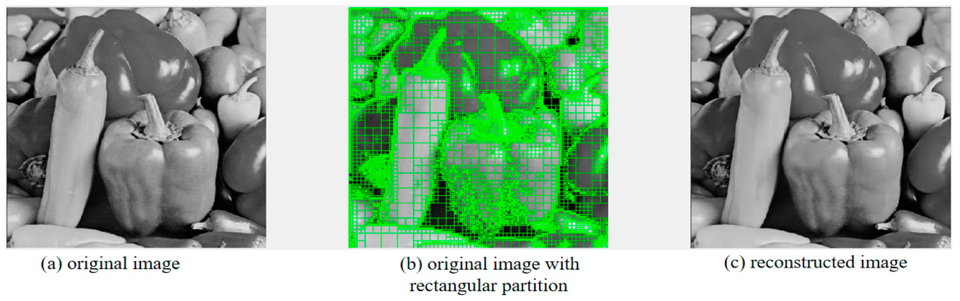
• We propose utilizing the adaptive non-uniform rectangular partition algorithm to segment images into non-overlapping D-blocks guided by local textures and features. This approach results in D-blocks of varying sizes and categorizes based on block dimensions, ultimately effectively reducing the pool of D-blocks and matching scope while improving the compression ratio and match precision.
• We design and use the non-uniform partition algorithm to adaptively segment images into different-sized R-blocks. Small R-blocks reconstruct regions with complex textures, while large R-blocks reconstruct areas with smooth or straightforward textures. The variable block size can help compress images, reduce “block effects” more effectively, and improve image reconstruction quality and compression ratio.
• We propose a novel block similarity-matching algorithm that incorporates precomputing. This approach entails summing pixel values for each D-block before conducting the R-block similarity match. This approach avoids redundant calculations during the loop-matching process, reducing computational complexity and encoding time.

The subsequent sections of this paper are organized as follows. Section 2 provides a succinct overview of the fundamental methodologies associated with fractal image compression and non-uniform rectangular partition. Section 3 presents a comprehensive examination of the fractal image compression techniques predicated on adaptive non-uniform rectangular partition, accompanied by an in-depth analysis of our proposed algorithms. Section 4 thoroughly assesses the compression algorithms’ performance, examining a range of parameters and presenting the associated experimental results. Finally, Section 5 outlines the conclusions drawn from this study.

2. The Fractal Image Compression and Non-Uniform Rectangular Partition

Fractal image compression utilizes images’ self-similarity and local repetition to significantly reduce data volume by storing pattern descriptors instead of individual pixel values. The non-uniform partition adapts to the varying characteristics across different image regions. Segmenting images into flexible blocks of various sizes and shapes effectively captures subtle changes, especially in areas with complex textures or irregular structures, thus markedly enhancing data compression efficiency.

2.1. Fractal Image Compression

The fractal image compression algorithm primarily relies on the iterative function system (IFS) and the collage theorem [19] to construct a fractal representation of images. This algorithm analyzes local similarities within an image while searching for suitable affine transformations. It then establishes corresponding fractal codes to minimize discrepancies between the original image and its fractal reconstruction. Fractal image compression coding aims to identify a series of compression mappings for a given image, thereby creating an IFS that closely approximates the original image by retaining its key parameters. In this context, the BFIC algorithm can be roughly divided into three stages: image segmentation, compressed affine transformation, and decoding reconstruction, as shown in Figure 1.

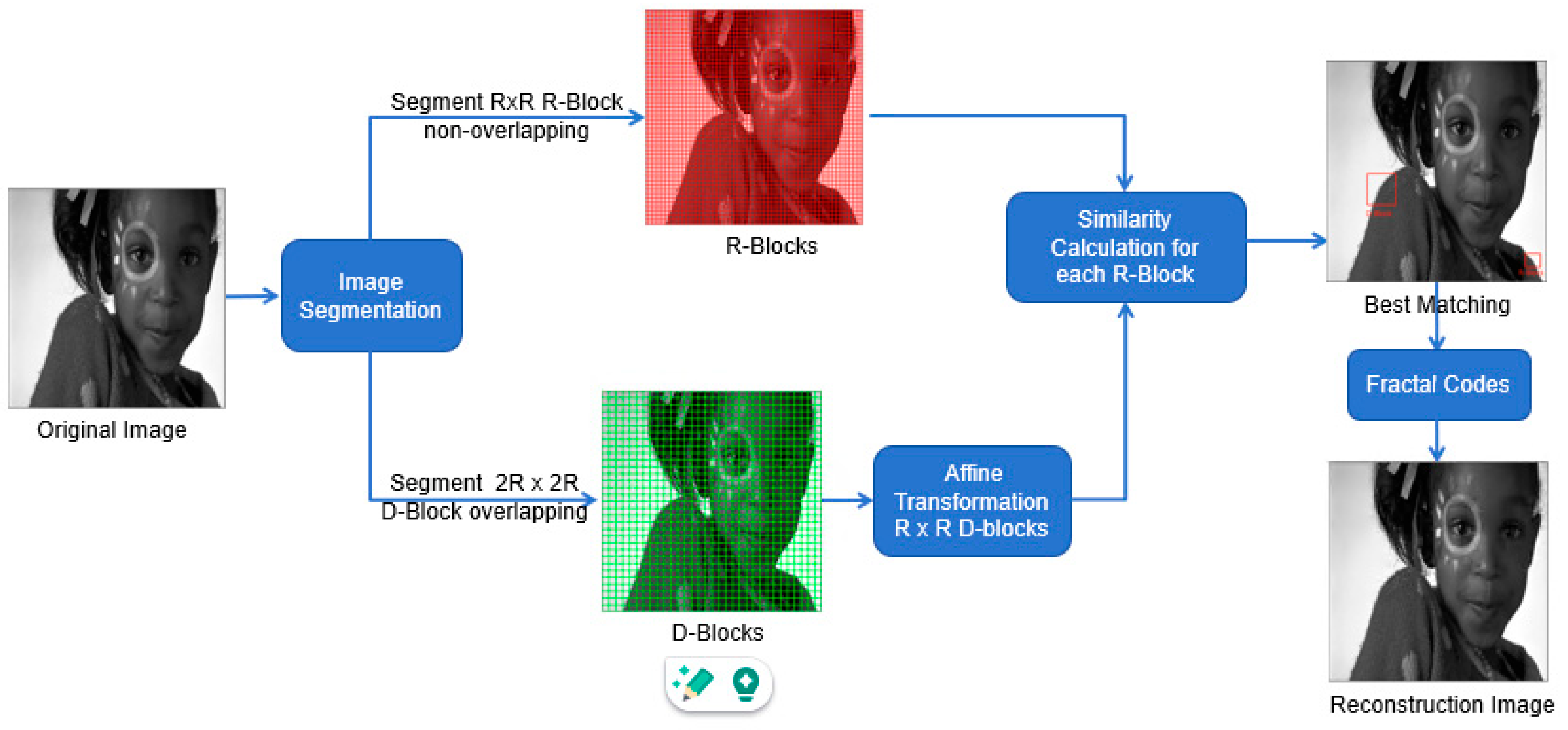
2.1.1. Image Segmentation

In the BFIC algorithms, a prevalent technique is utilizing a basic fixed-size block segmentation method. Here, the original image is partitioned into non-overlapping R-blocks and overlapping D-blocks. The R-blocks, segmented with dimensions R × R, form the encoded R-blocks. These blocks symbolize specific image regions intended for approximation via fractal coding. The desired compression ratio and the image characteristics determine the size of the R-blocks. Conversely, D-blocks are divided into dimensions D × D with a sliding step length of δ. A sliding window approach is employed horizontally and vertically across the image to generate these overlapping D-blocks.

In general, the size of the D-block is four times larger than the R-block (D = 2R), which facilitates a more flexible and precise matching process. The sliding step length δ (δ = R) dictates the overlap between contiguous D-blocks and influences the pool of D-block density. A smaller step length yields a larger pool of D-blocks with more potential transformations, whereas a larger step length results in a denser pool of D-blocks with fewer alternatives. During the encoding phase, each R-block is juxtaposed against the D-blocks to identify the most visually similar match. The affine transformation parameters that align the best matching D-block with the R-block are meticulously recorded.

2.1.2. Affine Transformation

The encoding stage of fractal compressive affine transformation can be conceptualized as a process involving spatial compression, isometric transformation, and grayscale matching search. Regarding spatial compression, the size of the D-blocks must be decreased to match that of the R-blocks for a proportional comparison. This is typically achieved using standard technologies, such as pixel averaging and undersampling methods, as depicted in Figure 2.

The isometric transformation guarantees that the fundamental geometric properties of the D-blocks are preserved despite resizing. This maintains the self-similar characteristics vital for fractal image compression coding. To enhance the quality of image reconstruction, we employed eight distinct isometric transformations, denoted as $t_i$(i = 0, 1, $\cdots$, 7), to augment the pool of D-blocks. These include the following:

(1)

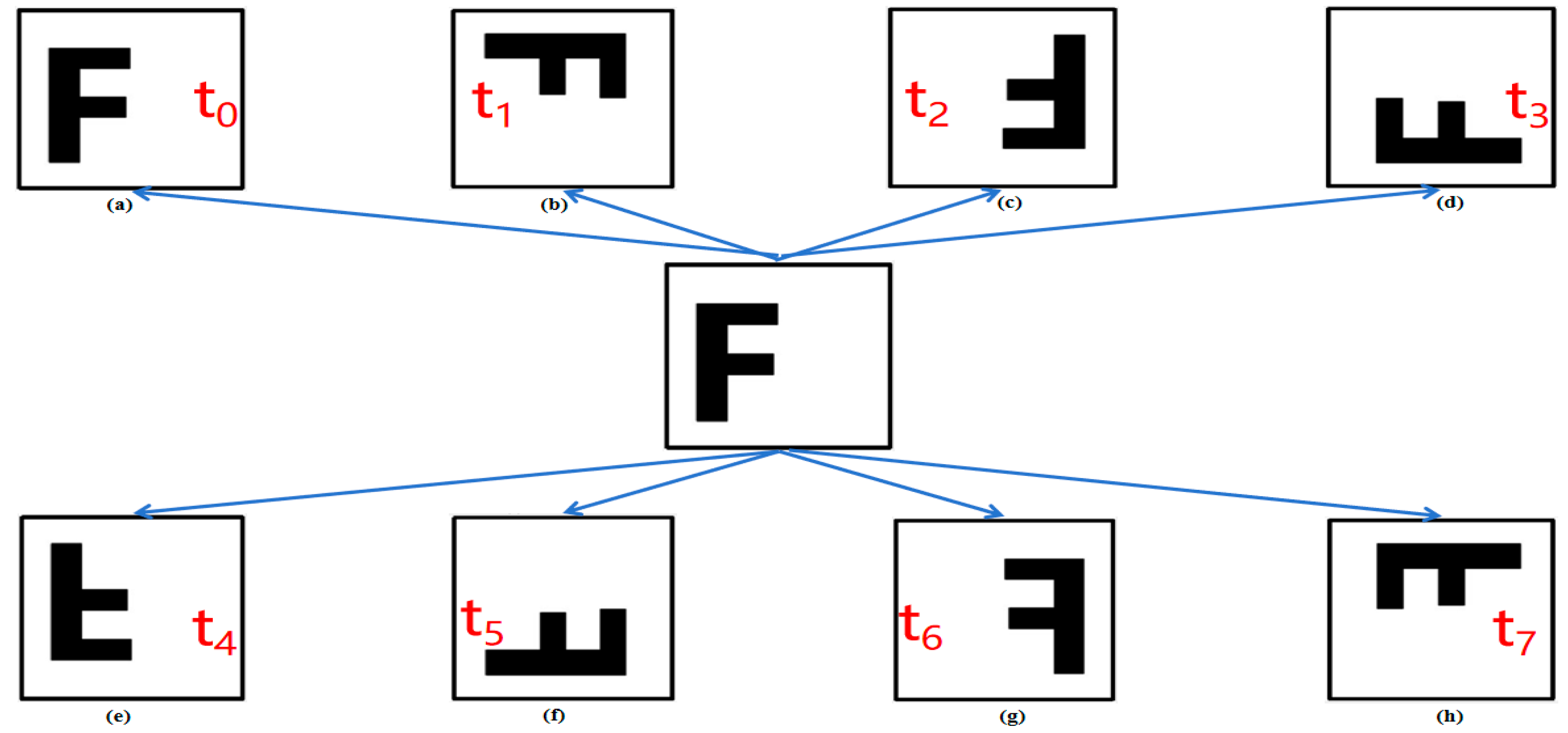
Identity transformation $t_0$: ${(t_0 D)}_{i,j}=D_{i,j}$, as shown in Figure 3a.

(2)

Rotate 90 degrees clockwise $t_1$: ${(t_1 D)}_{i,j}=D_{j,r-1-i}$, as shown in Figure 3b.

(3)

Rotate 180 degrees clockwise $t_2$: ${(t_2 D)}_{i,j}=D_{r-1-i,r-1-j}$, as shown in Figure 3c.

(4)

Rotate 270 degrees clockwise $t_3$: ${(t_3 D)}_{i,j}=D_{r-1-i,j}$, as shown in Figure 3d.

(5)

Symmetric reflection on x $t_4$: ${(t_4 D)}_{i,j}=D_{i,r-1-j}$, as shown in Figure 3e.

(6)

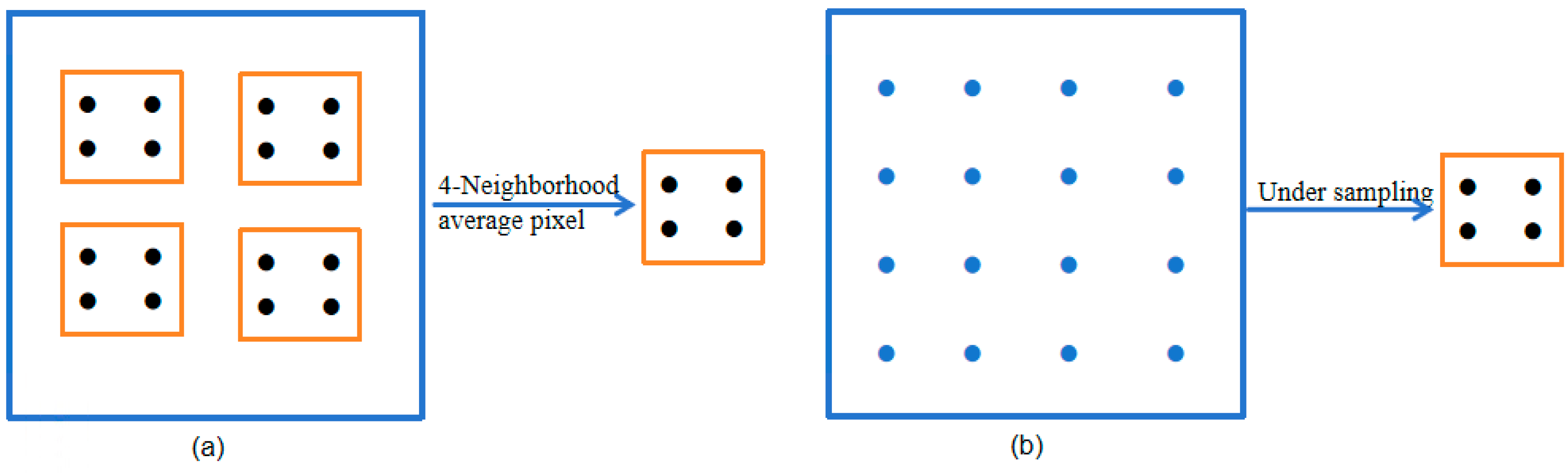
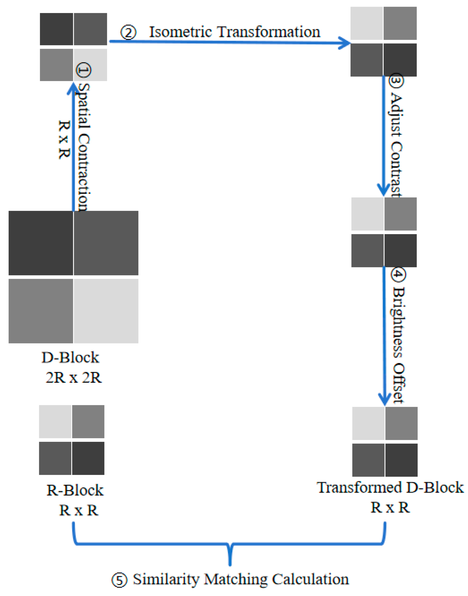
Symmetric reflection on y = x $t_5$: ${(t_5 D)}_{i,j}=D_{r-1-i,j}$, as shown in Figure 3f.

(7)

Symmetric reflection on y $t_6$: ${(t_6 D)}_{i,j}=D_{j,i}$, as shown in Figure 3g.

(8)

Symmetric reflection on y = −x $t_7$: ${(t_7 D)}_{i,j}=D_{r-1-j,r-1-i}$, as shown in Figure 3h.

Finally, a grayscale matching search is performed on each R-block to find the best matching D-block, as well as the corresponding contrast factor Fs and brightness offset coefficient Fo, so that the R-block and the best matching D-block meet the following grayscale transformations.

$$R=Fs·D+Fo·I$$

(1)

Simultaneously, they meet the minimum matching error, i.e., the following:

$$E\left(R,D\right)=min|| R-(Fs·D+Fo·I){||}^2 (Fs,Fo\in \mathrm{R})$$

(2)

where ||·|| represents an L2-norm and $I$ is a constant block with grayscale values of 1. Using the least squares method (LSM) to solve $E(R,D)$, we can obtain the following:

$$\left\{\begin{array}{c}Fs={\displaystyle \frac{〈R-\overline{R}·I, D-\overline{D}·I〉}{{‖D-\overline{D}·I‖}^2}}\\ Fo=\overline{R}-Fs·\overline{D}\end{array}\right.$$

(3)

where $〈·,·〉$ represents the Euclidean inner product $\overline{R}$ and $\overline{D}$ represent the mean of the gray pixel of R-blocks and D-blocks, respectively. If $‖D-\overline{D}·I‖=0$, then Fs = 0 and Fo = $\overline{R}$. So, the fractal codes for the R-block include the coordinate position of the D-block (Dtx, Dty), isometric transformation Tw, contrast factor Fs, and brightness offset coefficient Fo. Therefore, the reconstruction structure of the fractal codes is Fs, Fo, Tw, Dtx, and Dty. The detailed compression affine transformation process is shown in Figure 4.

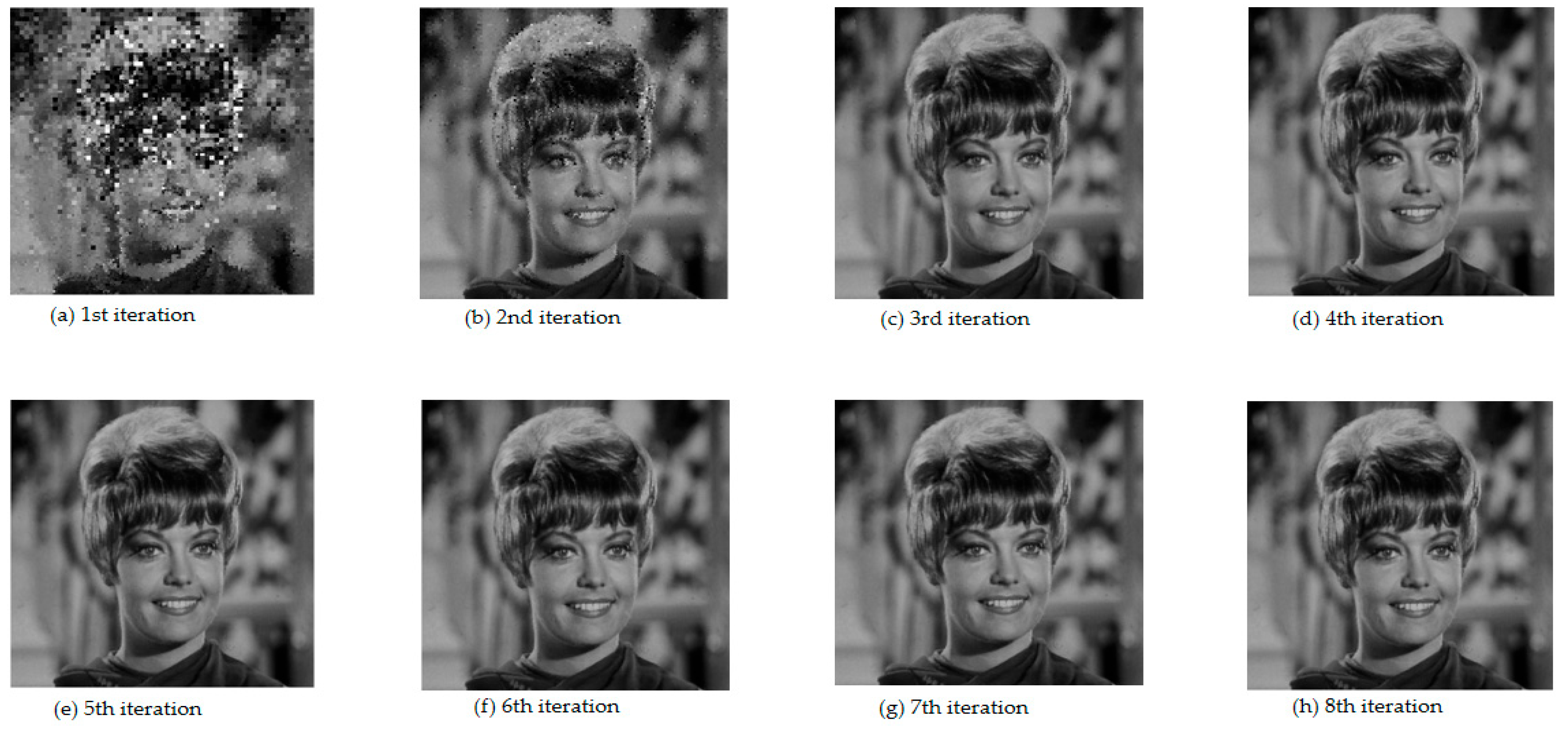
2.1.3. Decoding and Reconstruction

The process of decoding and reconstruction adheres to the iteration and collage method, starting from an arbitrary initial image, denoted as ${\mu }_0$, and executing N iterations as directed by a predetermined fractal code. The image that has been reconstructed, labeled as ${\mu }_{fix}$, can be considered an approximate fixed point of the compression transformation W, as outlined by the fractal codes. This mathematical model is represented as follows:

$$\begin{gathered} W^N{\mu }_0\approx \underset{n\to \infty }{\mathit{lim}}{W}^n{\mu }_0={\mu }_{fix} \\ {\mu }_{fix}\approx {\mu }_{org} \end{gathered}$$

(4)

In each iteration, the functional relationship between $R_i^{\left(k\right)}$ and its best matching block $D_{m\left(i\right)}^{(k-1)}$ is as follows:

$$\left\{\begin{array}{c}{R}_i^{\left(k\right)}={Fs}_i·{Tw}_k°S\left(D_{m\left(i\right)}^{(k-1)}\right)+{Fo}_i·I\\ D_{m\left(i\right)}^{\left(0\right)}=D_{m\left(i\right)}\end{array}\right.$$

(5)

After fractal image compression encoding, the generated fractal codes are used for image reconstruction. After 8–10 iterations, the image reconstruction quality remained stable, and there was no significant change in the reconstruction image’s PSNR. The following is the transformation process of the Zelda image generated in the first eight iterations, and the iterative reconstruction process is shown in Figure 5.

2.2. The Non-Uniform Rectangular Partition

The non-uniform partition is a digital signal processing and reconstruction technique that includes non-uniform rectangular and triangular partitions based on the configuration of the partition grid. The concept and methodology of non-uniform partitions were introduced in 1971 by A.V. Oppenheim et al. [26]. They proposed an algorithm utilizing the Fast Fourier Transform (FFT) to compute the Z-transform of non-uniformly distributed sampling points on the unit circle. This laid the groundwork for spectrum analysis with non-uniform spectral accuracy via the Non-uniform Discrete Fourier Transform (NDFT) [27]. The NDFT operates on the principle of non-uniform spectrum sampling and allows flexibility in selecting the position of the sampling point on the Z plane. Subsequent developments have introduced various methods of non-uniform partition, such as the Non-uniform Discrete Fourier Transform (NDFT) [28], Non-uniform Wedgelet Decomposition (NWD) [29], Non-Uniform Rectangular Partition (NURP) [30], and Non-Uniform Triangle Partition (NUTP) [31]. Furthermore, Zhang et al. proposed an image compression and reconstruction algorithm known as APUBT3-NUP [32], rooted in a non-uniform rectangular partition and U-system. This algorithm’s adaptive partitioning capability enhances the capture of image textures and features, yielding a superior compression ratio and reconstruction quality compared to traditional JPEG methods. Chen et al. [33] proposed using deep learning for fine-grained visual image processing and adaptive segmentation of image blocks to extract features. These discoveries underscore the unique advantages and potential applications of the non-uniform partition concept.

Practical evidence supports the efficacy of the non-uniform rectangle partition algorithm in adaptively dividing images of varying sizes based on local textures and features, utilizing the self-similar partition rule. This allows for rapid image reconstruction with enhanced quality. The methodology is rooted in the concept of least square approximation [34] via a polynomial function, which improves signal quality. Given a predetermined control threshold and initial region partition, the digital signal can be adaptively subdivided into diverse sizes, showcasing different textures and features, guided by the self-similar partition rule. This non-uniform partition approach has widespread applications in digital signal processing, including curve reconstruction [35], image representation [36], image compression [37], image denoising [38], image fusion [39], image super-resolution [40], information steganography [41], and image watermarking [42].

In the adaptive non-uniform rectangular partition algorithm context, three critical parameters influence any dimensional signal’s partitioning efficiency and reconstruction accuracy. First, the initial partition scheme is crucial, as variations in initial partitions can alter the configuration of partition grids and subsequently impact reconstruction parameters. Second, the predefined control threshold significantly affects the number of partition times and directly affects reconstruction quality. Finally, the polynomial function, which utilizes the least squares method (LSM) to determine polynomial coefficients, is instrumental in defining fitting accuracy. Notably, Formula (6) is invariably selected.

$$f(x,y)=ax+by+cxy+d \mathrm{or} f(x,y)=ax+by+c$$

(6)

The following example will describe how the process of adaptive non-uniform rectangular partition works. Suppose an image $G_m$ is regarded as a two-dimensional function over a rectangular domain. $Q\left({ x}_j,y_j\right)$ = $f_m\left(x_{j, }{ y}_j\right)$, $Q\left({ x}_j,y_j\right)$ denotes the grayscale value of the pixel of the sub-region, $\left(x_{j, }{ y}_j\right)$ ∈ $G_m$, where $x_{j }$and ${ y}_j$ represent the coordinates corresponding to pixel grayscale values. According to the self-similarity partition rule, during the initialization phase, the image $G_m$ will be divided into four sub-regions, recorded as $G_0$, $G_1$, $G_2$, and $G_3$. Then, for each sub-region, the current region is divided into four sub-regions based on the self-similarity rules, and this process is repeated until the current region’s MSE (mean square error) is lower than the preset control threshold. When a sub-region is designated as $G_m$, the positive integer $m$ serves as its identifier within a quaternary numbering system, as depicted in Figure 6; this quaternary representation encodes the hierarchical position and structural relationship of the sub-region within the self-similar partition process.

Similarly, the sub-regions obtained by non-uniform rectangular partition, according to the principle of the quadtree, assign numbers $m=m_k{4}^k+m_{k-1 }{4}^{k-1}+\cdots \cdots +m_1{4}^1+{m^{0}4}^0$.

$$m={\left(m_k{m}_{k-1}{\cdots \cdots m}_1{m}_0\right) }_4, m_j\in \left\{0,\right.\left.1,2,3\right\}, \mathrm{j}=0, 1, 2, \cdots \cdots , \mathrm{k}$$

(7)

The position and size of the required sub-regions can be quickly found based on the numbers, facilitating the least squares method for approximation calculations and image reconstruction operations. As shown in Figure 6c, the numbers p, q, r, and s are subdivided quadtree partition codes, such as r = 112, which can be traced from $G_1\to G_{11}\to G_{112}$ to their specific location. Finally, Figure 7 shows an example of using the adaptive non-uniform rectangular partition algorithm for image reconstruction.

3. Methodology and Algorithm Analysis

The fractal image compression algorithm uniformly segments blocks during the encoding phase, resulting in fixed-sized R-blocks and overlapping D-blocks. Notably, the dimensions of the segmentation block have significant implications for the algorithm’s encoding duration, reconstruction fidelity, and overall compression effectiveness. Using smaller block segmentation improves reconstruction quality; however, it may negatively affect the compression ratio and extend encoding time, potentially leading to redundancy and loss of inherent structural image information. Conversely, larger block segmentation might reduce reconstruction quality, resulting in noticeable “block effects” within the reconstructed images.

The adaptive non-uniform rectangular partition is defined by its capability to adjust to various features across different regions of an image. Segmenting images into flexible blocks of diverse sizes and shapes effectively captures subtle changes, particularly in areas with intricate textures or irregular structures, thus significantly enhancing data compression efficiency. During the encoding phase, the adaptive non-uniform rectangular partition method guides the division of R-blocks and D-blocks, promoting a more precise alignment with diverse image content. This is especially evident when dealing with feature vectors from R-blocks compared to D-blocks, utilizing distance metrics and least squares approximation. Such integration not only aids in identifying the most appropriate D-block but also minimizes redundancy, shortens encoding times, and improves the quality of the reconstructed images.

Gao et al. proposed an image compression encryption method featuring strong diffusion and an efficient chaotic mapping mechanism. They utilized 2D Logistic Rulkov neural [43] mapping and 3D-MCM [44] applied to the block matching algorithm during the non-uniform rectangle segmentation process to enhance the compression effect and encryption strength. The merger of fractal image compression and adaptive non-uniform rectangular partition demonstrates an impressive balance between image compression and maintaining visual fidelity during reconstruction. This method shows superior performance and offers broader practical applications.

3.1. Block Segmentation Method

Most fractal image compression techniques employ uniform segmentation methods to divide the original image (N × N) into R-blocks of R × R and overlapping D-blocks of 2R × 2R. The total number of D-blocks can be calculated using the following formula: ((N − 2R)/R + 1) × 4 × ((N − 2R)/R + 1). Additionally, when applying eight different isometric transformations, they create a composite pool of D-blocks Ω, containing 8 × ((N − 2R)/R + 1) × 4 × ((N − 2R)/R + 1) blocks. Many D-blocks result in significant time spent on optimal matching calculations. Furthermore, the segmentation scheme of R-blocks in fractal image compression methods is crucial for the image’s encoding time, compression ratio, and reconstruction quality. As shown in Figure 8, the number of R-blocks in three different algorithms significantly impacts the image’s PSNR, compression ratio (CR), and encoding time (ET). It should be noted that smaller R-blocks, with a larger quantity, typically yield a higher PSNR at the expense of a lower CR and increased ET. In contrast, larger R-blocks correspond to fewer R-blocks, allowing for shorter encoding times and greater compression ratios (CRs). Still, they can lead to a decline in image quality (PSNR).

We introduce and employ the adaptive non-uniform rectangular partition method to address the previously mentioned limitation. This technique divides the original image into non-overlapping D-blocks and R-blocks of varying sizes based on the local texture found within the image. For the same reconstruction quality, the number of R-blocks and D-blocks produced using this method is significantly lower than that in BFIC. Consequently, this results in a substantial reduction in encoding time and an enhancement in the compression ratio. The adaptive non-uniform rectangular partition algorithm establishes a predetermined range for block sizes. The image is segmented into non-overlapping D-blocks with dimensions of 8 × 8, 16 × 16, and 32 × 32. At the same time, it is partitioned into R-blocks measuring 4 × 4, 8 × 8, and 16 × 16.

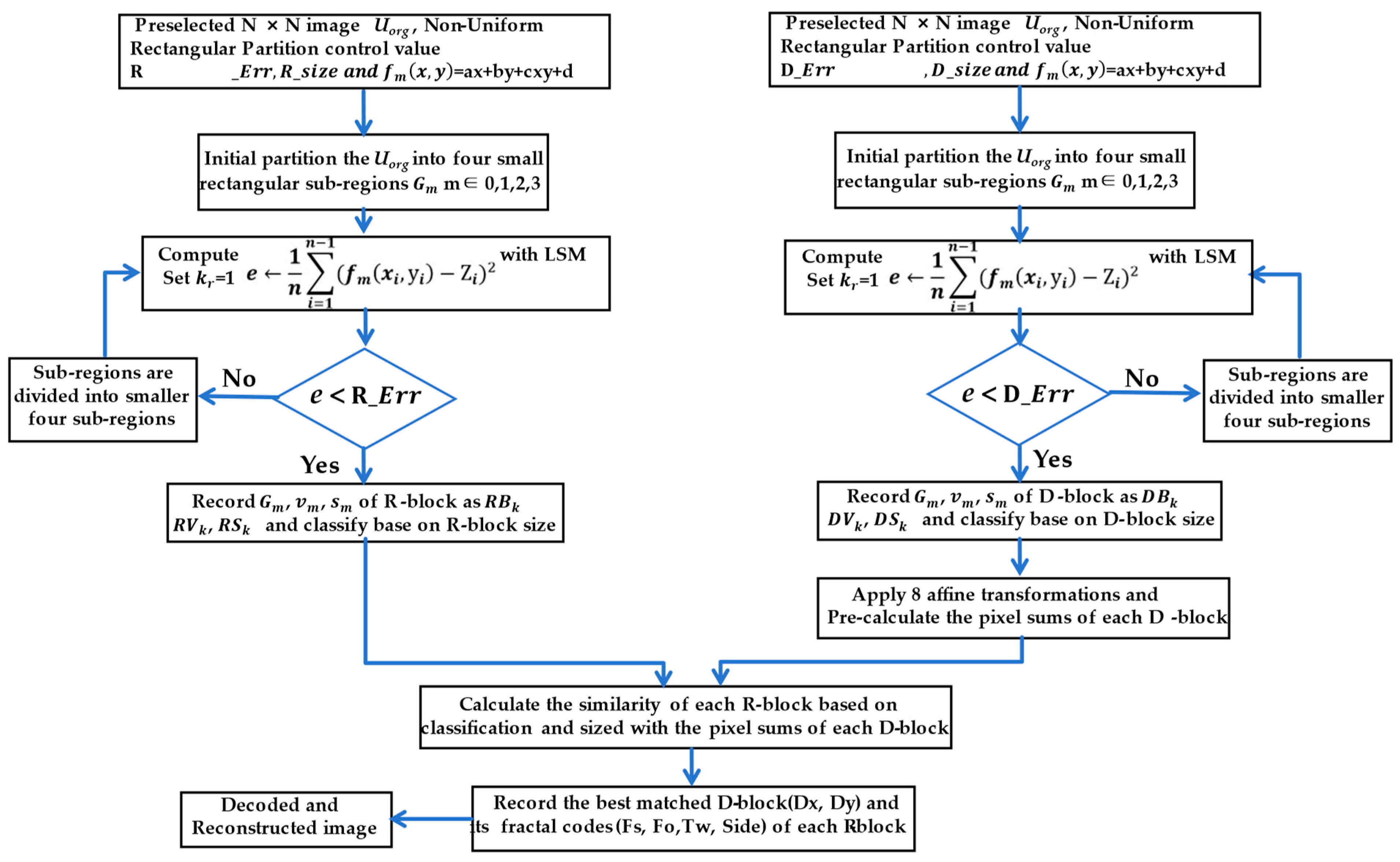
3.2. Process of the FICANRP Scheme

The non-uniform partition method provides significant advantages in image segmentation and feature representation. FICANRP begins by applying an adaptive non-uniform rectangular partition scheme to the original image, dividing it into variable-sized R-blocks and D-blocks. Next, eight isometric transformations and the precomputation of the sum are applied to each D-block. Finally, a localized optimal matching computation generates the fractal codes. A comprehensive flowchart illustrating the core algorithmic procedure is included to understand our proposed methodology better, as shown in Figure 9. This diagram clearly outlines the sequential steps of fractal image compression using the adaptive non-uniform rectangular partition approach.

3.3. Algorithm Details

As can be seen from Formula (3), the traditional R-block matching algorithm suffers from significant computational inefficiency due to the repeated summation of D-blocks during similarity calculations, which occurs four times. This issue arises because each D-block must undergo eight isometric transformations, necessitating independent computations of similarity metrics. The cumulative effect of these redundant operations results in a substantial increase in computational complexity. This bottleneck is particularly pronounced in real-time applications, like video compression, where latency directly affects performance. The FICANRP algorithm addresses this by precomputing and reusing pixel sums, thus eliminating redundant operations while maintaining matching accuracy. Pixel value sums for all D-blocks are precalculated during initialization and stored in a temporary table indexed by each block’s spatial coordinates and dimensions. At runtime, similarity matching retrieves these precomputed sums in constant time, avoiding iterative recalculations.

In the R-block and D-block similarity matching process, the computational complexity of calculating the pixel sum for each D-block is given by Equation (8). Suppose an N × N image is divided into $Nr$ R × R R-blocks and $Nd$2R × 2R D-blocks, respectively. The time complexity of computing the pixel sums for all D-blocks in the traditional fractal image compression algorithm can be expressed as follows:

$$O\left(T\right)=O\left(\left(Nr\times Nd\times 8\right)\times 4\right)=O(({\displaystyle \frac{N\times N}{R\times R}})\times ({\displaystyle \frac{N\times N}{2R\times 2R}})\times 8\times 4)=8({{\displaystyle \frac{N}{R}})}^4$$

(8)

Here, factor 8 corresponds to the eight possible transformations (rotation and intensity changes) applied to each D-block during the matching process. In contrast, factor 4 represents the sum of the D-block in Formula (3), which needs to be calculated four times. Therefore, the overall computational complexity increases linearly with the number of R-blocks and D-blocks.

Using the precomputation method of D-block pixel summation, the complexity of the FICANRP algorithm is calculated as follows:

$$O\left(T\right)=O(Nd\times 8)=8 Nd =4(({{\displaystyle \frac{N}{R}})}^2)$$

(9)

It accelerates similarity calculations by orders of magnitude. The algorithm significantly reduces computational overhead by eliminating redundant recalculations, making it especially suitable for real-time systems such as video compression.

3.4. Algorithm Description

The FICANRP algorithm entails partitioning the image into non-uniform rectangular blocks in the segmentation and encoding phase. Subsequently, a contractive transformation function is constructed for each R-block, representing the image as a series of fractal codes. The following provides a detailed description of Algorithm 1.

Algorithm 1: The FICANRP encoding algorithm

Input: Size N × N$\mathrm{Image} { \mu }_{org}$ Output: Fractal codes (Fs, Fo, Tw, R_size, Dtx, Dty) Algorithm process: 1. Preset the non-uniform partition control threshold R_Err, D_Err, and the range of R-block size and D-block size. 2. Apply the adaptive non-uniform rectangular partition algorithm on image ${\mu }_{org}$, to obtain different sizes of R-blocks and D-blocks, respectively. 3. /* k is the sub-region code / 4. Set k = 1 5. Initial partition the ${\mu }_{org}$ into four small rectangular sub-regions $G_m$, m ∈ 0,1,2,3 6. Compute Vk, Sk, Bk with ENCODING ($G_m$) 7. Function ENCODING ($G_m$) 8. Set the top left vertex of $G_m$ as Vm, the size of $G_m$ as Sk, the grey value of $G_m$as Bk 9.  For each pixel point ($x_i$, $y_i$) in $G_m$ do 10.    Compute $f_m(x_i$, $y_i$) ← $a_m{x}_i$+ $b_m{y}_i$+ $c_m{x}_i{y}_i$+ $d_m$ with LSM 11.   /* $z_i$ is the gray value of the pixel in the sub-region / 12.    Compute e ← ${\displaystyle \frac{1}{n}}\sum _{i=1}^{n-1}{\left(f_m\right(x_i,y_i)-z_i)}^2$ 13.   Endfor 14.   If e < R_Err or Sk ≤ min R-block size/e < D_Err or Sk ≤ min D-block size 15.    Record Gm, Vm, Sm of R-block/D-block, as Bk, Vk, Sk, 16.    Classify Bk based on block size. 17.   Else 18.    Compute ENCODING (Gmr), r ∈ 0, 1, 2, 3 19.   End if 20. End Function 21. Perform the average of 4-neighborhood pixel values for each D-block to obtain the compression transformation D’-block. Then, perform eight isometric transformations and various summations with block pixels to form the pool Ω of D-blocks. 22. Preprocess calculations by summing up the pixel values of the D-block before each R-block similarity match. 23. According to the partition order of R-block, calculate the similarity coefficient $E(R_i,D_k)$ of R-block and D-block, the smaller the $E(R_i,D_k)$, the more similar it is, then record the fractal codes of each R-block where the $E(R_i,D_k)$ is smallest. 24. After all R-blocks are matched, the corresponding image reconstruction of fractal codes Fs, Fo, Tw, R_size, Dtx, and Dty will be obtained.

In the decoding and reconstruction phase, iterative techniques systematically deform, concatenate, and fuse subgraphs across various scales while adhering to the non-uniform distribution pattern. This approach ensures high-fidelity image reconstruction with minimal redundancy. The primary steps in this phase are outlined in Algorithm 2.

Algorithm 2: The FICANRP decoding algorithm

Input: Fractal codes (Fs, Fo, Tw, R_size, Dtx, Dty) Output: Decoding reconstruction Image ${\mu }_{fix}$ Algorithm process: 1. Preset the maximum iteration number N, read the fractal codes information, and extract data from fractal encoding files, including the IFS parameter set (Fs, Fo, Tw, R_size, Dtx, Dty) of each R-block. 2. Initialize decoding space and create two buffers the same size as the original image: an R-region buffer and a D-region buffer. 3. Initialize an arbitrary image matrix I_New, the same size as the original, to reconstruct the decoded image.  For n = 1:N/* n represents the iteration number/   For Nr = 1: Tprn /* Tprn represents the number of R-block/     Dx = Dtx(Nr)     Dy = Dty (Nr)       /* For each R-block R(Nr), locate the best match D-block D(Nr)/     D(Nr) = I_New(Dx + 2R_size: Dy + 2R_size)     /* Apply spatial compression Ts and isometric transformation Tw to D(Nr)/     Temp(Nr) = Tw (Ts(D(Nr)))     I_New(Nr) = Fs(Nr) $\times$ Temp(Nr) + Fo(Nr)     Nr = Nr + 1   End for  End for 4. Update the decoding area, copy and paste the content of the R-region image generated by the current iteration into the D-region, thereby updating the content of the entire decoded image. 5. Check if the number of iterations N has reached the preset maximum n. If so, end the iteration process; If not, return to step (2) to continue with the next iteration. Generally, the number of iterations is 8–10 times, and the reconstruction quality of the image will reach its optimal level.

The integration of fractal image compression and adaptive non-uniform rectangular partitioning allows for flexible adaptation to the diverse characteristics of various image regions, thereby enhancing encoding efficiency while maintaining a certain level of quality in the reconstructed images.

4. Simulation Experiments and Results

Our study primarily focuses on evaluating the efficiency of image compression and reconstruction through experimental simulation. We compare the Basic Fractal Image Compression (BFIC) and quadtree fractal image compression (QFIC) schemes. Additionally, we conducted a thorough comparative analysis using the methodology proposed in this paper.

4.1. Experimental Conditions and Key Parameters

All methods are implemented in the MATLAB R2016a environment. The experiments were conducted on a system equipped with an Intel i5-9500 CPU @ 3.0 GHz, 12 GB of RAM, and a Windows 10 Professional 64-bit operating system. The software environment is configured carefully to ensure the consistency and reliability of the experimental results. Specifically, the Image Processing Toolbox in MATLAB is utilized to support essential image processing functions and tools. All algorithms are executed under default MATLAB settings unless specific parameters are adjusted to meet the requirements of individual methods. For evaluation, we selected five widely used standard 8-bit grayscale images—Zelda, Peppers, Plane, Girl, Cameraman, Kodim12 and Kodim20—each with a resolution of 512 × 512 pixels, along with Kodim21 and Kodim24 from the Kodak dataset, which has a resolution of 1024 × 1024 pixels, as test images. These benchmark images are commonly used in image processing experiments and are widely recognized in fractal image compression algorithm research, providing a reliable basis for performance comparison.

The simulation experiment described below is designed for data analysis in fractal image compression, using an adaptive non-uniform rectangular partition. The critical parameter for the partition control threshold, represented as R_Err/D_Err, significantly influences the image segmentation of R-blocks and D-blocks, including their size and quantity. Additionally, it impacts key performance indicators, such as the peak signal-to-noise ratio (PSNR), encoding time (ET), and the compression ratio (CR). As illustrated in Figure 10, as the partition control threshold R_Err decreases, the image is divided into more R-blocks, thereby enhancing the reconstruction quality. However, this also necessitates more parameters for reconstruction, which reduces the compression ratio and extends the encoding time. Therefore, setting the experimental parameter for the partition control threshold R_Err substantially affects the results.

In fractal image compression based on the adaptive non-uniform rectangular partition (FICANRP) framework, calculating R_Err is essential for assessing the quality of image compression and reconstruction. To effectively compute R_Err in scenarios where computational resources are limited or obtaining standard deviation values is difficult, we propose a simplified model that utilizes the image’s mean intensity (Me) and mean gradient (Mg). This model significantly decreases computational complexity while maintaining high accuracy in R_Err estimation.

We observed a strong linear relationship between R_Err, mean intensity, and mean gradient through experimental data analysis. Therefore, a linear regression model can effectively describe this relationship. R_Err can be expressed as a linear combination of mean intensity (Me) and mean gradient (Mg).

R_Err = 2.38Me + 2.95Mg − 280

(10)

4.2. Evaluation Standard

In fractal image compression, the compression ratio (CR) is a crucial metric for evaluating the effectiveness of the compression method. This ratio offers a quantitative measure of the data size reduction achieved through the encoding process that utilizes fractal properties. The formula for the compression ratio is CR = U/C, where U denotes the size of the original, uncompressed image data and C represents the size of the compressed image data. This metric is essential for assessing the performance and efficiency of fractal image compression.

The fractal codes Fs, Fo, and Tw used in fractal image compression are typically quantized into 5-bit, 7-bit, and 3-bit formats, respectively. In our proposed method, the fractal codes for an N × N image—Fs, Fo, Tw, R_size, Dtx, and Dty—are quantified as 5-bit, 7-bit, 3-bit, 2-bit, p-bit, and q-bit, respectively. Here, p and q are dynamically quantized based on the partition number of the D-block. Consequently, the compression ratio (CR) of the image is defined as follows:

CR = N × N × 8/(Num_R × (Fs + Fo+ Tw + R_size + p + q))

(11)

where Num_R represents the number of R-blocks and R_size characterizes the style of image segmentation into varying R-block sizes. It is important to note that the number of R-blocks and D-blocks is not fixed. Instead, the quantity of image blocks obtained will be dynamically adjusted based on the texture of the image and the partition control thresholds.

To evaluate the performance of our method, we introduce some basic metrics, such as the total encoding time and the PSNR of the reconstructed image. In our method, the PSNR is defined as follows:

$$PSNR=10\times {log}_{10}\left({\displaystyle \frac{{255}^2}{MSE}}\right)$$

(12)

where $MSE={\displaystyle \frac{1}{N}}{\sum }_{j=1}^N[z^{\prime }\left(x_{j,}{y}_j\right)-z\left(x_{j,}{y}_j\right){]}^2$. N denotes the number of pixels, $z\left(x_{j,}{y}_j\right)$ denotes the grayscale value of pixel within the original image, and $z^{\prime }\left(x_{j,}{y}_j\right)$ denotes the grayscale value of the pixel within the reconstructed image.

4.3. Algorithm Complexity

In the BFIC algorithm, the computational overhead primarily originates from exhaustive comparisons between fixed-size R-blocks and a large D-block pool. The complexity calculation for the pixel sum of the D-block is as follows:

$$O\left(T_1\right) =O(Nr\times Nd\times 8\times 4)=O(({\displaystyle \frac{N^2}{R^2}\times }{({\displaystyle \frac{N-2R}{R}}+1)}^2\times 8)\times 4)$$

(13)

The computational complexity of quadtree fractal image compression (QFIC) primarily stems from its hierarchical block matching mechanism between R-blocks and D-blocks. Three interdependent factors determine this complexity: First, the hierarchical block dimensions, where operations scale quadratically with the size of R-blocks and D-blocks; second, the reconstruction fidelity constraint imposed by R-blocks’ mean square error (R_mse); and finally, the quadtree segmentation depth governs the multi-resolution decomposition granularity. Suppose an image is divided into three layers, and the number of 16 × 16 R-blocks is ${Nr}_{16}$, the number of 8 × 8 R-blocks is ${Nr}_8$, and the number of 4 × 4 R-blocks is ${Nr}_4$. The corresponding number of 32 × 32 D-blocks is ${Nd}_{32}$, 16 × 16 D-blocks is ${Nd}_{16}$, and 8 × 8 D-blocks is ${Nd}_8$. The QFIC algorithm complexity for the pixel sum of the D-block is shown in Formula (14).

$$O\left(T_2\right) =O({Nr}_4\times {Nd}_8\times 8\times 4)+O({Nr}_8\times {Nd}_{16}\times 8\times 4)+O({Nr}_{16}\times {Nd}_{32}\times 8\times 4)$$

(14)

Since FICAURP uses an adaptive algorithm to segment R-blocks, the number of R-blocks will change dynamically according to the presetting of the non-uniform partition coefficient. Suppose FICAURP segments the original image into ${Nr}_{16}$ 16 × 16 R-blocks, ${Nr}_8$ 8 × 8 R-blocks, and ${Nr}_4$ 4 × 4 R-blocks. The corresponding number of 32 × 32 D-blocks is ${Nd}_{32}$. The number of 16 × 16 D-blocks is ${Nd}_{16}$. The number of 8 × 8 D-blocks is ${Nd}_8$. Using the precomputing and reusing algorithm to sum the D-block pixel value, its computational complexity is as follows:

$$O\left(T_3\right)=O(Nr\times Nd\times 8)=O({Nd}_8\times 8)+O({Nd}_{16}\times 8)+O({Nd}_{32}\times 8)$$

(15)

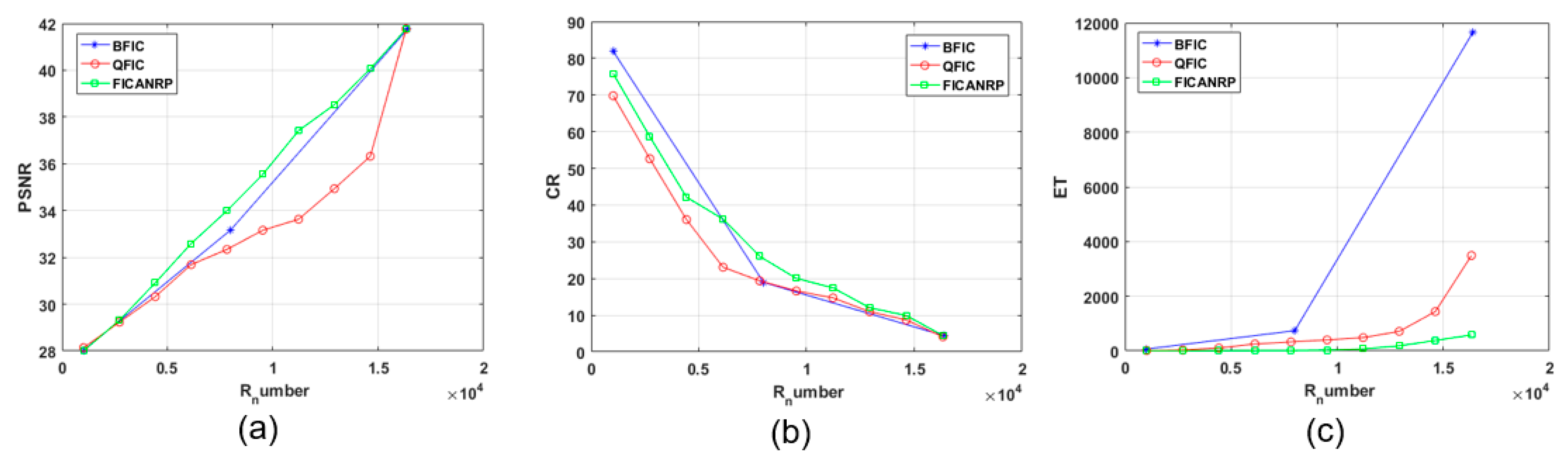
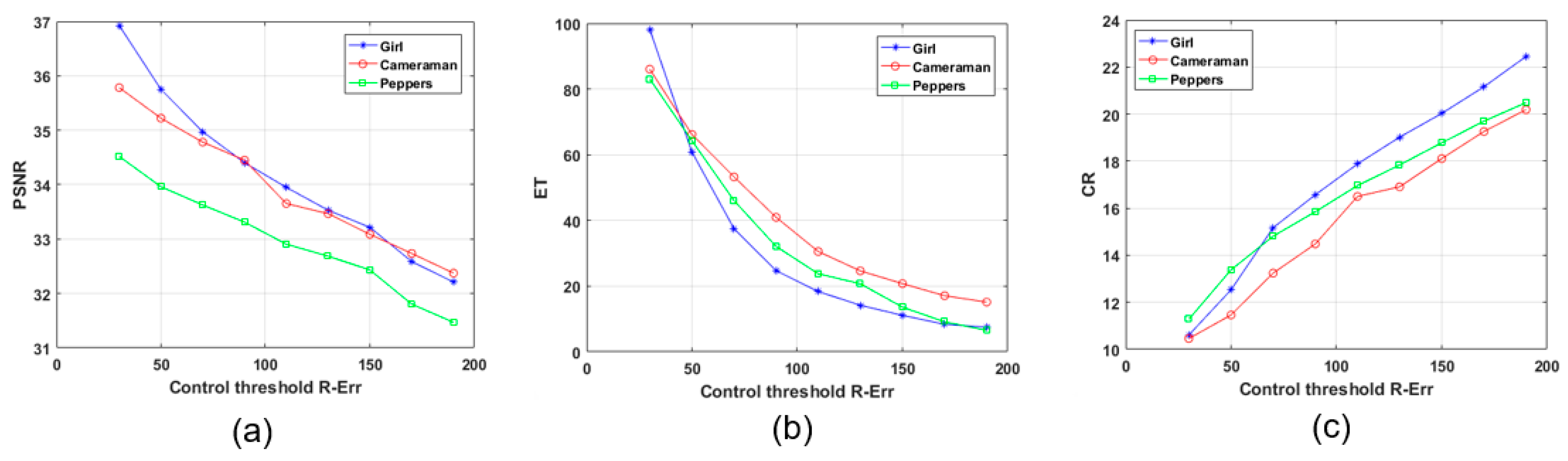
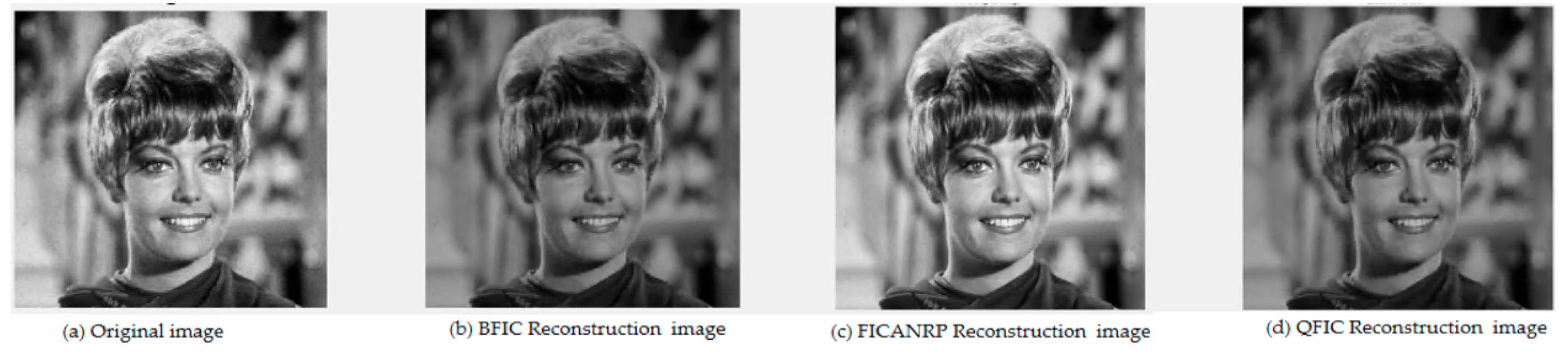
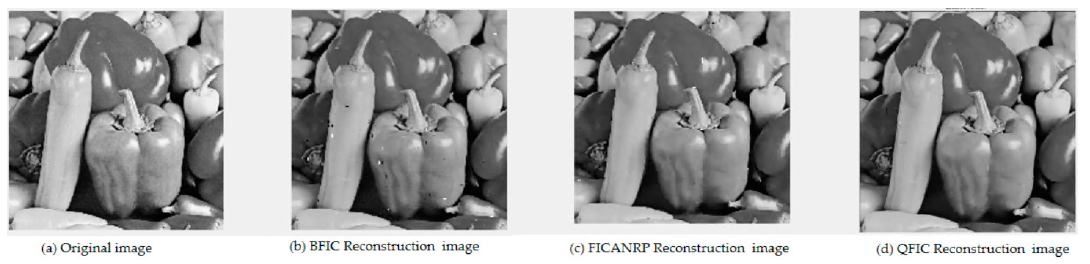
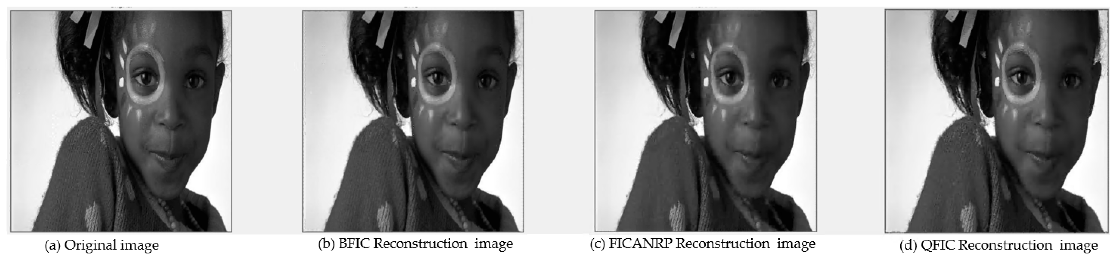
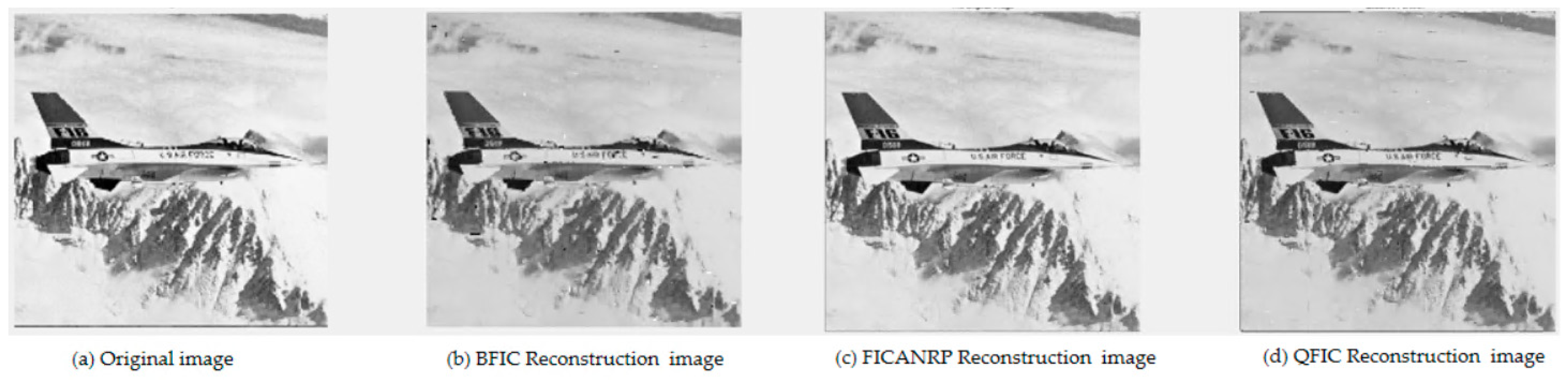
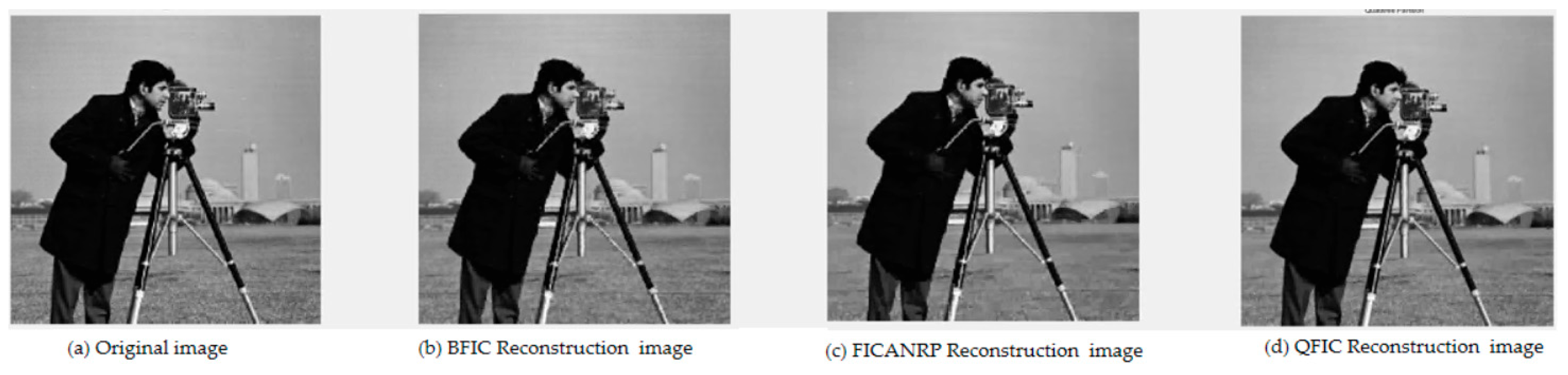
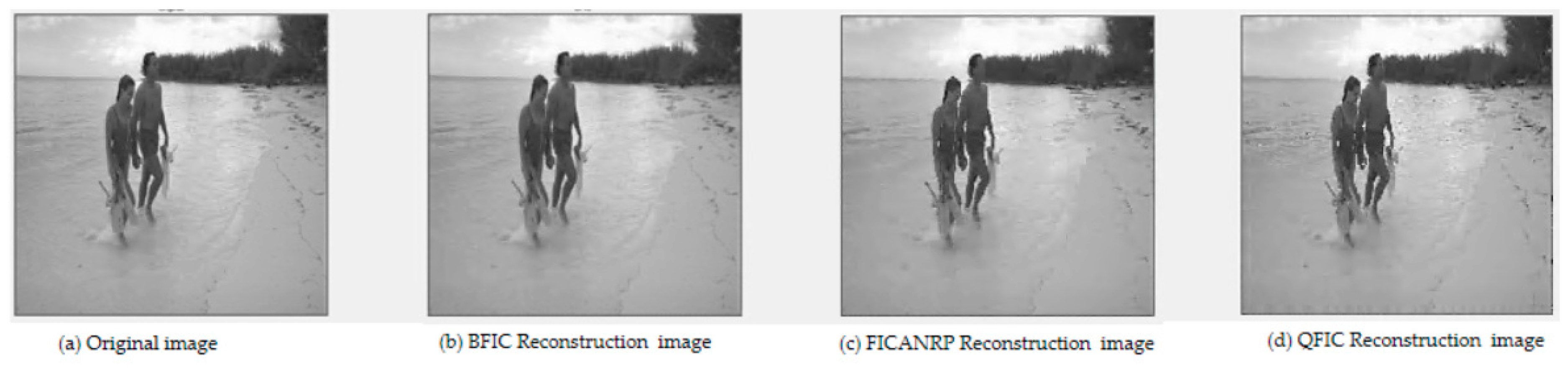
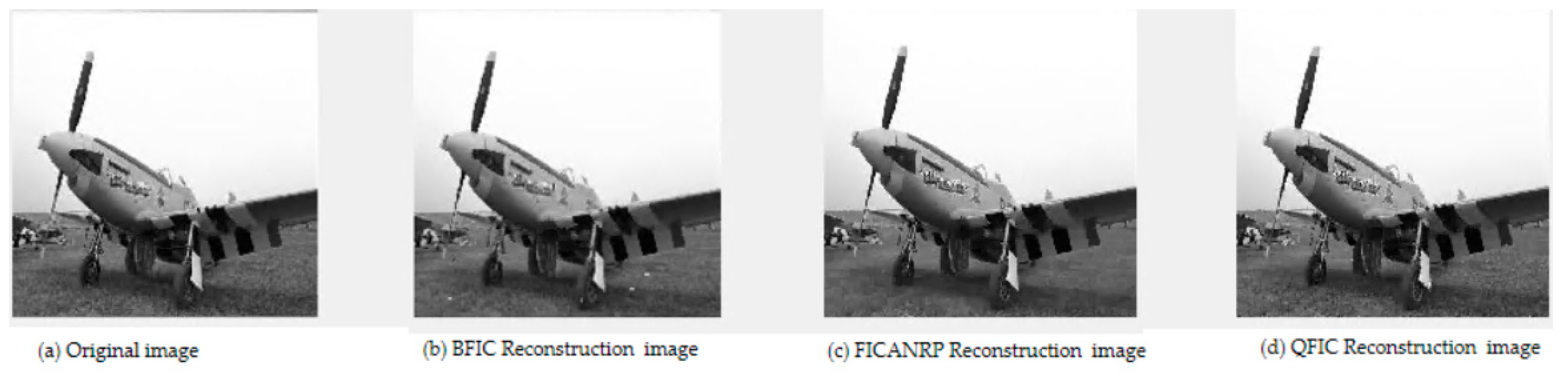
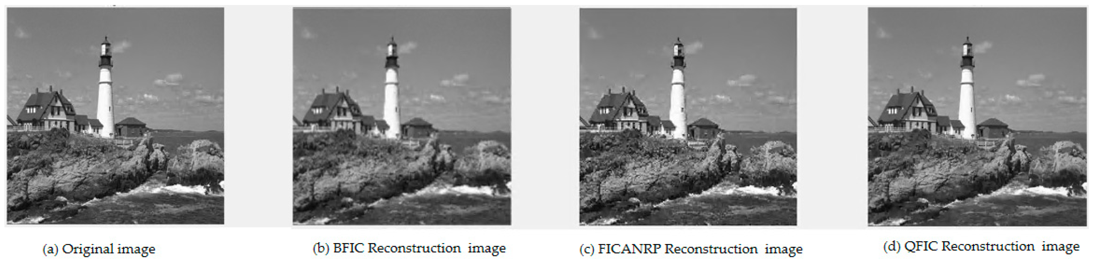
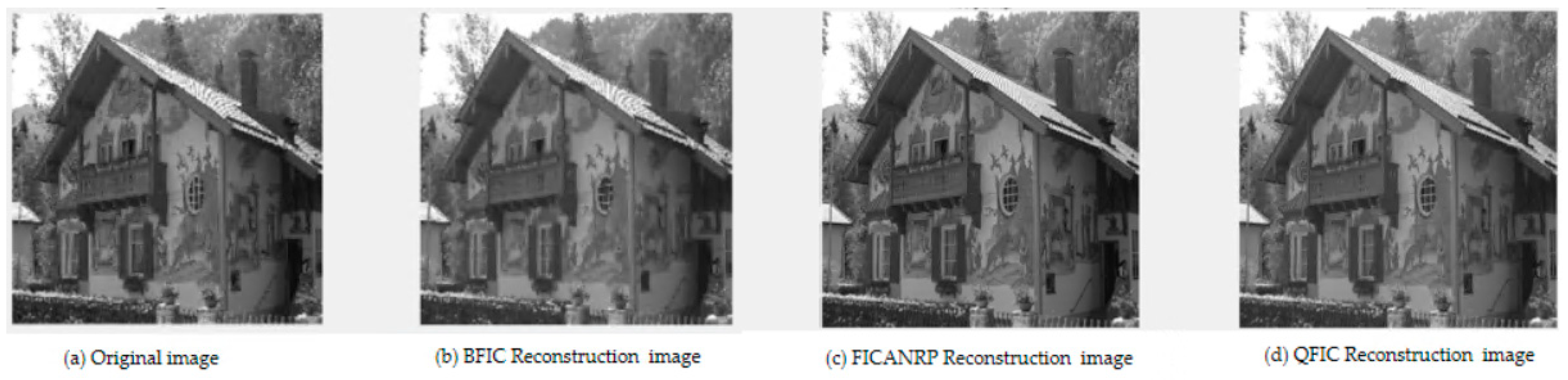
4.4. Analysis and Results of the Experiment

In our comparative analysis condition, the BFIC approach partitions the original image into 4096 non-overlapping R-blocks using a fixed 8 × 8 grid size. Simultaneously, an overlapping segmentation method employing a 16 × 16 grid with an eight-unit step size is implemented, resulting in 3969 D-blocks. After the D-blocks’ post-affine transformation, a comprehensive search and matching process is conducted on each R-block. The Fs, Fo, Tw, Dtx, and Dty fractal codes are quantized using 5-bit, 7-bit, 3-bit, 6-bit, and 6-bit resolutions, respectively. The resulting image compression ratio (CR) is as follows:

CR = 512 × 512 × 8/(4096 × (5 + 7 + 3 + 6 + 6)) = 18.96

(16)

The QFIC [11] results are based on the following conditions: the minimum R-block size is 4 × 4, and the reconstructed R-block’s mean square error (R_mse) is established at 50. The original image is initially divided into non-overlapping 16 × 16 R-blocks and overlapping 32 × 32 D-blocks. Subsequently, a classification scheme is implemented for all D-blocks, organizing them into three major categories and 24 subcategories to reduce the number of domains relative to a range. The next step involves calculating the best match between each R-block and D-block, selecting the one with the smallest error, and comparing it with the R_mse. If the R_mse exceeds 50 and the R-block size is larger than 4 × 4, the R-block is divided into four smaller blocks until the R_mse is less than 50 or the R-block size is less than or equal to 4 × 4. The fractal codes of Fs, Fo, Tw, Ql, Dtx, and Dty are quantized as 5-bit, 7-bit, 3-bit, 1-bit, 6-bit, and 6-bit, respectively. Here, the Ql denotes the depth of the quadtree segmentation.

As shown in

Table 1. Performance comparison of test images under different fractal algorithms.

Image	Algorithm	PSNR	ET (s)	Num_R	Num_D	CR	R_Err	R_MSE	O(T)
	BFIC	35.86	749.47	4096	3969	18.96	\	\	5.2 × 108
	QFIC	34.82	269	3055	16,129	22.88	\	50	2.4 × 107
Zelda	FICANRP	36.10	13.45	3895	424	20.05	70	\	3.4 × 103
	BFIC	29.73	751.91	4096	3969	18.96	\	\	5.2 × 108
	QFIC	30.06	397.40	4141	16,129	16.88	\	50	7.7 × 107
Peppers	FICANRP	31.12	6.15	3673	295	21.10	200	\	3.4 × 103
	BFIC	31.20	720.52	4096	3969	18.96	\	\	5.2 × 108
	QFIC	30.93	530.04	4945	16,129	13.68	\	50	2.8 × 108
Girl	FICANRP	32.10	12.76	3838	751	20.23	180	\	6.0 × 103
	BFIC	24.54	762.56	4096	3969	18.96	\	\	5.2 × 108
	QFIC	25.07	690.16	5848	16,129	11.95	\	50	3.9 × 108
Plane	FICANRP	29.35	10.51	3895	424	19.94	420	\	3.4 × 103
	BFIC	30.99	733.08	4096	3969	18.96	\	\	5.2 × 108
	QFIC	32.30	567.72	5095	16,129	13.70	\	50	2.4 × 108
Cameraman	FICANRP	32.34	14.17	3847	538	20.19	200	\	4.3 × 103
	BFIC	32.13	767.14	4096	3969	18.96	\	\	5.2 × 108
	QFIC	29.95	452.82	4267	16,129	15.85	\	50	2.2 × 109
Kodim12	FICANRP	32.85	8.68	3991	349	19.46	200	\	1.1 × 104
	BFIC	27.37	751.26	4096	3969	18.96	\	\	5.2 × 108
	QFIC	30.71	560.70	5047	16,129	13.40	\	50	2.6 × 108
Kodim20	FICANRP	31.72	12.82	3655	475	21.25	200	\	1.5 × 104
	BFIC	31.06	12,575.00	16,384	16,130	17.66	\	\	8.5 × 109
Kodim21	QFIC	31.80	6948.04	22,639	65,025	16.70	\	50	5.4 × 109
(1024 × 1024)	FICANRP	32.26	112.20	15,640	1312	18.50	220	\	1.1 × 104
	BFIC	29.48	12,466.00	16,384	16,130	17.66	\	\	8.5 × 109
Kodim24	QFIC	29.58	7045.00	23,533	65,025	11.50	\	50	5.8 × 109
(1024 × 1024)	FICANRP	30.17	117.34	15,157	1558	19.08	220	\	1.2 × 104

In Table 1, PSNR stands for peak signal-to-noise ratio; ET stands for encoding time, and its measurement unit is seconds, and CR stands for compression ratio. Num_R denotes the total number of R-blocks, Num_D denotes the total number of D-blocks, R_mse denotes the mean squared error of the R-block reconstructed, R_Err denotes the partition control threshold, and O(T) represents the algorithm complexity.

, the FICANRP scheme significantly improves the efficiency of fractal image compression coding and reconstruction quality compared to BFIC and QFIC, which effectively preserve critical image details while requiring fewer R-blocks for reconstruction. The FICANRP demonstrates superior performance metrics, with average improvements of 1.425 in the compression ratio (CR), 1.51 dB in the peak signal-to-noise ratio (PSNR), and an encoding acceleration factor of 67.44 relative to the BFIC baseline. Notably, the performance enhancement observed in processing the Peppers test image is impressive, where the algorithm achieves a remarkable 122-fold speed improvement in encoding, along with a 1.39 dB PSNR gain and a CR of 21.10, representing a 2.14-fold enhancement over BFIC’s compression capability. These substantial improvements stem from the optimized partitioning mechanism that dynamically adjusts block dimensions based on local texture complexity, effectively balancing computational load with reconstruction fidelity.

However, our method shows a performance gap compared to GPU-based fractal compression techniques that leverage parallel processing [17]. For instance, when encoding the Barbara image at the highest achievable PSNR level, the GPU-accelerated Fisher method—implemented on an NVIDIA GeForce GT 660 M GPU using 4 × 4 R-blocks—finishes the encoding process in 366.67 s, while our method takes 473 s. This discrepancy underscores the significant acceleration achieved through hardware-level parallelism in GPU-based implementations. Nevertheless, our method exhibits competitive performance under certain conditions, particularly at lower PSNR levels, where the computational burden is reduced and the balance between speed and reconstruction quality remains favorable.

As shown in

Table 2. Performance comparison of test images under the QFIC and FICANRP algorithms.

Image	Algorithm	PSNR	ET(s)	Num_R	Num_D	CR	R_Err	R_mse
	QFIC	34.82	269	3055	16,129	22.88	\	50
Zelda	FICANRP	34.83	7.22	3271	343	23.75	200	\
	QFIC	30.06	397.4	4141	16,129	16.88	\	50
Peppers	FICANRP	30.14	6.15	2902	298	26.76	185	\
	QFIC	30.93	530.04	4945	16,129	13.68	\	50
Girl	FICANRP	30.97	8.19	3155	712	24.61	330	\
	QFIC	25.07	690.16	5848	16,129	11.95	\	50
Plane	FICANRP	25.80	6.01	2500	280	31.07	400	\
	QFIC	32.30	567.72	5095	16,129	13.7	\	50
Cameraman	FICANRP	32.34	14.17	3847	538	20.19	200	\
	QFIC	29.95	452.82	4267	16,129	15.85	\	50
Kodim12	FICANRP	29.95	6.5	2344	301	33.13	450	\
	QFIC	30.71	560.7	5047	16,129	13.4	\	50
Kodim20	FICANRP	30.77	8.2	3085	376	25.18	350	\
Kodim21	QFIC	31.80	6948.04	16,493	65,025	16.7	\	50
(1024 × 1024)	FICANRP	31.92	107.21	15,040	1312	19.23	250	\
Kodim24	QFIC	29.58	7045	23,533	65,025	11.50	\	50
(1024 × 1024)	FICANRP	30.17	117.34	15,157	1558	19.08	250	\

, the comparison between QFIC and FICANRP under identical PSNR conditions shows significant performance improvements achieved by the proposed FICANRP method. Regarding encoding time (ET), FICANRP demonstrates considerable speedups across all tested images. For instance, the encoding time for the Girl image is reduced from 530.04 s with QFIC to just 8.19 s with FICANRP, representing a speedup factor of approximately 64.72×. The improvement is even more pronounced for the Plane image, where the ET decreases dramatically from 690.16 s to only 6.01 s—an impressive acceleration factor of 114.83×. Similarly, the encoding times for the Peppers and Kodim21 images are reduced from 397.4 to 6.15 s and from 6948.04 to 107.21 s, respectively, corresponding to speedup factors of 64.62× and 64.81×. These results illustrate the superior computational efficiency of FICANRP.

In addition to the significant reductions in encoding time, FICANRP also achieves notable improvements in the compression ratio (CR). For example, the CR for the Girl image increases from 13.68 with QFIC to 24.61 with FICANRP—a 79.91% enhancement. More impressively, for the Plane image, the CR rises from 11.95 using QFIC to 31.07 with FICANRP, representing a 159.96% increase, indicating a more efficient representation of image content. Similar improvements are observed with the Peppers and Zelda images, where the CR goes from 16.88 to 26.76 (58.53%) and from 22.88 to 23.75 (3.8%), respectively.

Table 2’s comparative data indicates that the compression ratio of certain images (e.g., Kodim21 and Zelda) does not change significantly, as the texture complexity and structure of the images directly influence the compression ratio. Low-complexity images (such as solid colors and the sky) can achieve high compression ratios due to substantial data repetition, clear edges, and redundant information; however, high-complexity images (like natural landscapes and facial photos) have limited compression potential and lower compression ratios owing to intricate details, random pixel variations, and less redundant information.

The proposed precomputing algorithm has shown noteworthy improvements in the efficiency of block similarity matching calculations, particularly in reducing computational complexity and encoding time. As indicated in

Table 3. Encoding time of test images with or without precomputing algorithms.

	ET(s) Without Precomputing		ET(s) With Precomputing
	BFIC	FICANRP	BFIC	FICANRP
Zelda	749.47	73.33	292.23	13.45
Peppers	751.91	33.55	298.56	6.15
Girl	720.52	80.13	281.63	12.76
Plane	762.56	56.08	292.69	10.51
Cameraman	733.08	69.89	299.38	14.17
Kodim21 (1024 × 1024)	12,575.00	762.27	4857.90	112.20

, the encoding time (ET) for both the BFIC and FICANRP algorithms has been significantly decreased through D-block pixel sum precomputing. Specifically, the BFIC algorithm achieves a 2.6-fold speedup, while the FICANRP algorithm shows an even greater acceleration of approximately 5 times compared to their respective versions without precomputing.

For instance, the encoding time for the Zelda image using BFIC decreases from 749.47 s without precomputing to 292.23 s with precomputing, representing a 2.56× speedup. Similarly, the FICANRP algorithm reduces the encoding time from 73.33 s to 13.45 s, achieving a 5.45× acceleration. This trend is consistent across other test images. For the Peppers image, BFIC’s ET drops from 751.91 s to 298.56 s (2.52× speedup), while FICANRP’s ET decreases from 33.55 s to 6.15 s (5.45× speedup). The same pattern is observed for the Girl image, where BFIC’s ET reduces from 720.52 s to 281.63 s (2.56× speedup) and FICANRP’s ET decreases from 60.05 s to 11.26 s (5.33× speedup). Notably, for larger images, such as Kodim21 (1024 × 1024), the benefits of precomputing become even more evident. BFIC’s ET is reduced from 12,575 s to 4857.90 s (2.59× speedup), while FICANRP’s ET decreases from 762.27 s to 112.2 s (6.80× speedup). These substantial reductions in encoding time can be attributed to the core strategy of precomputing various pixel sum values for each D-block that has undergone eight isometric transformations. We effectively reduce memory access latency during the matching process by storing these precomputed results in a temporary table constructed according to the block coordinates and sizes.

Experiments show that this precomputation and optimization approach significantly enhances computational efficiency without compromising accuracy. The block similarity matching process becomes more effective, as the algorithm can retrieve precomputed pixel sum values instead of recalculating them repeatedly. Consequently, the overall performance of both BFIC and FICANRP algorithms improves, making them more suitable for real-time applications that demand fast and accurate image compression.

On the other hand, subjective visual analysis evaluates the performance of BFIC and QFIC, and our proposed method in reconstructing images focuses on human perception of image quality. As shown in Figure 11, Figure 12, Figure 13, Figure 14, Figure 15, Figure 16, Figure 17, Figure 18 and Figure 19, the reconstructed images are visually assessed regarding detail preservation, color fidelity, contrast, and the presence of artifacts. The images reconstructed using the BFIC method show “block effects” in areas with rich local texture features, which observers especially notice in complex regions, such as edges and delicate patterns. Moreover, white noise points emerge in more severe cases, further degrading the visual experience and causing the images to appear less natural to the human eye. In contrast, the images reconstructed using the QFIC method show color distortion, with a noticeable darkening of colors and reduced contrast. These images lack depth and structural hierarchy, making it challenging to distinguish subtle changes in shadows and textures. Additionally, when these reconstructed images are magnified for observation, evident block effects and white noise become apparent. Conversely, the method proposed in this article produces visually appealing effects, enhances the preservation of image textures, and achieves a more natural color reconstruction.

In summary, based on the analysis and comparison of the experimental results, it is evident that the proposed FICANRP method employs a non-uniform partition strategy during image segmentation, enabling a more effective separation of D-blocks and R-blocks according to the local texture characteristics of the image. This approach allows for high-quality image reconstruction using fewer R-blocks, improving the overall image compression ratio. Furthermore, the precomputation of D-block pixel sums significantly reduces the computational complexity of matching block similarity calculations, resulting in an acceleration of over five times and a substantial reduction in encoding time. Objective comparisons with the BFIC and QFIC methods demonstrate that the proposed FICANRP method achieves superior image compression efficiency and reconstruction quality while requiring less encoding time. From a subjective visual perspective, the reconstructed images produced by our method exhibit more realistic and natural color reproduction, along with better preservation of fine texture details, leading to a more visually pleasing outcome.

5. Conclusions and Future

This study presents the FICANRP scheme as a solution to the high computational complexity and long encoding times associated with traditional BFIC and QFIC methods. This is achieved by segmenting images into variable-sized R-blocks based on an adaptive non-uniform rectangle partition guided by local textures and features, which requires fewer R-blocks for image reconstruction while maintaining the same PSNR. Furthermore, the FICANRP method uses non-overlapping block segmentation to reduce the D-block pool. It also employs a novel block similarity matching algorithm, significantly lowering the algorithm’s complexity and encoding time. The experimental results indicate that the proposed approach effectively balances computational efficiency, reconstruction quality, and compression performance, making it an ideal choice for applications requiring rapid encoding and efficient storage. Moreover, the proposed scheme can be adapted to various application scenarios by fine tuning parameters to meet specific requirements of the reconstructed image, such as the peak signal-to-noise ratio (PSNR), compression ratio (CR), or encoding time (ET).

Although FICANRP has significantly improved compared to traditional fractal image compression methods, it still faces certain limitations. In particular, when processing images with weak self-similarity or complex structures, the matching accuracy may be compromised, resulting in a peak signal-to-noise ratio (PSNR) lower than modern transform-based or deep learning-based compression techniques. Moreover, the current implementation of FICANRP does not incorporate deep learning or machine learning strategies to assist with segmentation or similarity matching. This limits its ability to fully leverage recent technological advancements, especially in emerging applications, such as remote sensing and medical imaging. Future research could potentially enhance this method by optimizing segmentation algorithms, integrating deep learning techniques designed for rapid similarity matching of image block features, or adapting it to the fields of remote sensing and medical imaging with appropriate modifications.

In the future, FICANRP will undergo a more in-depth comparison with commonly used compression methods, like JPEG, to highlight our compression performance further. This will involve metrics such as the PSNR, the compression ratio, and encoding time across various image types and application scenarios to optimize the algorithm and better meet diverse practical application needs.

References

- Barnsley, M.F. Fractals Everywhere, 2nd ed.; 3. [Print.]; Morgan Kaufmann: San Diego, CA, USA, 1993. [Google Scholar]
- Jacquin, A.E. Image coding based on a fractal theory of iterated contractive image transformations. IEEE Trans. Image Process. 1992, 1, 18–30. [Google Scholar] [CrossRef] [PubMed]
- Barnsley, M.F.; Demko, S. Iterated function systems and the global construction of fractals. Proc. R. Soc. Lond. Math. Phys. Sci. 1985, 399, 243–275. [Google Scholar] [CrossRef]
- Tong, C.S.; Wong, M. Adaptive approximate nearest neighbor search for fractal image compression. IEEE Trans. Image Process. 2002, 11, 605–615. [Google Scholar] [CrossRef]
- Tan, T.; Yan, H. The fractal neighbor distance measure. Pattern Recognit. 2002, 35, 1371–1387. [Google Scholar] [CrossRef]
- Wang, X.-Y.; Wang, Y.-X.; Yun, J.-J. An improved fast fractal image compression using spatial texture correlation. Chin. Phys. B 2011, 20, 104202. [Google Scholar] [CrossRef]
- Jaferzadeh, K.; Kiani, K.; Mozaffari, S. Acceleration of fractal image compression using fuzzy clustering discrete-cosine-transform-based metric. Image Process. IET 2012, 6, 1024–1030. [Google Scholar] [CrossRef]
- Wang, J. A Novel Fractal Image Compression Scheme With Block Classification and Sorting Based on Pearson’s Correlation Coefficient. IEEE Trans. Image Process. 2013, 22, 3690–3702. [Google Scholar] [CrossRef]
- Jaferzadeh, K.; Moon, I.; Gholami, S. Enhancing fractal image compression speed using local features for reducing search space. Pattern Anal. Appl. 2017, 20, 1119–1128. [Google Scholar] [CrossRef]
- Cao, J.; Zhang, A.; Shi, L. Orthogonal sparse fractal coding algorithm based on image texture feature. IET Image Process. 2019, 13, 1872–1879. [Google Scholar] [CrossRef]
- Fisher, Y. Fractal Image Compression: Theory and Application; Springer Science & Business Media: Berlin/Heidelberg, Germany, 1995. [Google Scholar]
- Wang, X.-Y.; Guo, X.; Zhang, D.-D. An effective fractal image compression algorithm based on plane fitting. Chin. Phys. B 2012, 21, 090507. [Google Scholar] [CrossRef]
- Li, W.; Pan, Q.; Lu, J.; Li, S. Research on Image Fractal Compression Coding Algorithm Based on Gene Expression Programming. In Proceedings of the 2018 17th International Symposium on Distributed Computing and Applications for Business Engineering and Science (DCABES), Wuxi, China, 19–23 October 2018; pp. 88–91. [Google Scholar]
- Smriti, S.; Laxmi, A.; Hima, B.M. Image Compression using PSO-ALO Hybrid Metaheuristic Technique. Int. J. Perform. Eng. 2021, 17, 998. [Google Scholar] [CrossRef]
- Tang, Z.; Yan, S.; Xu, C. Adaptive super-resolution image reconstruction based on fractal theory. Displays 2023, 80, 102544. [Google Scholar] [CrossRef]
- Varghese, B.; S., K. Parallel Computation strategies for Fractal Compression. In Proceedings of the 2020 2nd International Conference on Advances in Computing, Communication Control and Networking (ICACCCN), Greater Noida, India, 18–19 December 2020; pp. 1024–1027. [Google Scholar]
- Al Sideiri, A.; Alzeidi, N.; Al Hammoshi, M.; Chauhan, M.S.; AlFarsi, G. CUDA implementation of fractal image compression. J. Real-Time Image Process. 2020, 17, 1375–1387. [Google Scholar] [CrossRef]
- Li, L.-F.; Hua, Y.; Liu, Y.-H.; Huang, F.-H. Study on fast fractal image compression algorithm based on centroid radius. Syst. Sci. Control Eng. 2024, 12, 2269183. [Google Scholar] [CrossRef]
- Lin, Y.; Xie, Z.; Chen, T.; Cheng, X.; Wen, H. Image privacy protection scheme based on high-quality reconstruction DCT compression and nonlinear dynamics. Expert Syst. Appl. 2024, 257, 124891. [Google Scholar] [CrossRef]
- Zhang, Y.; Jia, C.; Chang, J.; Ma, S. Machine Perception-Driven Facial Image Compression: A Layered Generative Approach. IEEE Trans. Circuits Syst. Video Technol. 2025, 35, 3825–3836. [Google Scholar] [CrossRef]
- Song, J.; He, J.; Feng, M.; Wang, K.; Li, Y.; Mian, A. High Frequency Matters: Uncertainty Guided Image Compression with Wavelet Diffusion. arXiv 2024, arXiv:2407.12538. [Google Scholar] [CrossRef]
- Relic, L.; Azevedo, R.; Zhang, Y.; Gross, M.; Schroers, C. Bridging the Gap between Diffusion Models and Universal Quantization for Image Compression. arXiv 2025, arXiv:2504.02579. [Google Scholar]
- Afrin, A.; Mamun, M.A. A Comprehensive Review of Deep Learning Methods for Hyperspectral Image Compression. In Proceedings of the 2024 3rd International Conference on Advancement in Electrical and Electronic Engineering (ICAEEE), Gazipur, Bangladesh, 25–27 April 2024; pp. 1–6. [Google Scholar]
- Shen, T.; Peng, W.-H.; Shih, H.-C.; Liu, Y. Learning-Based Conditional Image Compression. In Proceedings of the 2024 IEEE International Symposium on Circuits and Systems (ISCAS), Singapore, Singapore, 19–22 May 2024; pp. 1–5. [Google Scholar]
- Kuang, H.; Ma, Y.; Yang, W.; Guo, Z.; Liu, J. Consistency Guided Diffusion Model with Neural Syntax for Perceptual Image Compression. In Proceedings of the 32nd ACM International Conference on Multimedia, Melbourne, VIC, Australia, 28 October–1 November 2024; pp. 1622–1631. [Google Scholar]
- Oppenheim, A.; Johnson, D.; Steiglitz, K. Computation of spectra with unequal resolution using the fast Fourier transform. Proc. IEEE 1971, 59, 299–301. [Google Scholar] [CrossRef]
- Bagchi, S.; Mitra, S.K. The nonuniform discrete Fourier transform and its applications in filter design. I. 1-D. IEEE Trans. Circuits Syst. II Analog Digit. Signal Process. 1996, 43, 422–433. [Google Scholar] [CrossRef]
- Bagchi, S.; Mitra, S.K. The nonuniform discrete Fourier transform and its applications in filter design. II. 2-D. IEEE Trans. Circuits Syst. II Analog Digit. Signal Process. 1996, 43, 434–444. [Google Scholar] [CrossRef]
- Donoho, D.L. Wedgelets: Nearly minimax estimation of edges. Ann. Stat. 1999, 27, 859–897. [Google Scholar] [CrossRef]
- Tak, U.K.; Tang, Z.; Qi, D. A non-uniform rectangular partition coding of digital image and its application. In Proceedings of the 2009 International Conference on Information and Automation, Zhuhai/Macau, China, 22–24 June 2009; pp. 995–999. [Google Scholar]
- Yuan, X.; Cai, Z. An Adaptive Triangular Partition Algorithm for Digital Images. IEEE Trans. Multimed. 2019, 21, 1372–1383. [Google Scholar] [CrossRef]
- Zhang, Y.; Cai, Z.; Xiong, G. A New Image Compression Algorithm Based on Non-Uniform Partition and U-System. IEEE Trans. Multimed. 2021, 23, 1069–1082. [Google Scholar] [CrossRef]
- Chen, H.; Zendehdel, N.; Leu, M.C.; Yin, Z. A gaze-driven manufacturing assembly assistant system with integrated step recognition, repetition analysis, and real-time feedback. Eng. Appl. Artif. Intell. 2025, 144, 110076. [Google Scholar] [CrossRef]
- Benouaz, T.; Arino, O. Least square approximation of a nonlinear ordinary differential equation. Comput. Math. Appl. 1996, 31, 69–84. [Google Scholar] [CrossRef]
- Zhao, W.; U, K.; Luo, H. Adaptive non-uniform partition algorithm based on linear canonical transform. Chaos Solitons Fractals 2022, 163, 112561. [Google Scholar] [CrossRef]
- Zhao, W.; U, K.; Luo, H. Image representation method based on Gaussian function and non-uniform partition. Multimed. Tools Appl. 2023, 82, 839–861. [Google Scholar] [CrossRef]
- U, K.; Ji, N.; Qi, D.; Tang, Z. An Adaptive Quantization Technique for JPEG Based on Non-uniform Rectangular Partition. In Future Wireless Networks and Information Systems; Zhang, Y., Ed.; Lecture Notes in Electrical Engineering; Springer: Berlin/Heidelberg, Germany, 2012; Volume 143, pp. 179–187. ISBN 978-3-642-27322-3. [Google Scholar]
- Song, R.; Li, Y.; Zhang, Q.; Zhao, Z. Image denoising method based on non-uniform partition and wavelet transform. In Proceedings of the 2010 3rd International Congress on Image and Signal Processing, Yantai, China, 16–18 October 2010; pp. 703–706. [Google Scholar]
- Liu, X.; Kintak, U. A novel multi-focus image-fusion scheme based on non-uniform rectangular partition. In Proceedings of the 2017 International Conference on Wavelet Analysis and Pattern Recognition (ICWAPR), Ningbo, China, 09–12 July 2017; pp. 53–58. [Google Scholar]
- Zhao, W.; U, K.; Luo, H. An image super-resolution method based on polynomial exponential function and non-uniform rectangular partition. J. Supercomput. 2023, 79, 677–701. [Google Scholar] [CrossRef]
- Wang, H.; Cheng, X.; Wu, H.; Luo, X.; Ma, B.; Zong, H.; Zhang, J.; Wang, J. A GAN-based anti-forensics method by modifying the quantization table in JPEG header file. J. Vis. Commun. Image Represent. 2025, 110, 104462. [Google Scholar] [CrossRef]
- U, K.; Hu, S.; Qi, D.; Tang, Z. A robust image watermarking algorithm based on non-uniform rectangular partition and DWT. In Proceedings of the 2009 2nd International Conference on Power Electronics and Intelligent Transportation System (PEITS), Shenzhen, China, 19–20 December 2009; pp. 25–28. [Google Scholar]
- Gao, S.; Zhang, Z.; Iu, H.H.-C.; Ding, S.; Mou, J.; Erkan, U.; Toktas, A.; Li, Q.; Wang, C.; Cao, Y. A Parallel Color Image Encryption Algorithm Based on a 2-D Logistic-Rulkov Neuron Map. IEEE Internet Things. J. 2025, 12, 18115–18124. [Google Scholar] [CrossRef]
- Gao, S.; Iu, H.H.-C.; Erkan, U.; Simsek, C.; Toktas, A.; Cao, Y.; Wu, R.; Mou, J.; Li, Q.; Wang, C. A 3D Memristive Cubic Map with Dual Discrete Memristors: Design, Implementation, and Application in Image Encryption. IEEE Trans. Circuits Syst. Video Technol. 2025, 1. [Google Scholar] [CrossRef]