

Analysis of Grid-Connected Damping Characteristics of Virtual Synchronous Generator and Improvement Strategies

Abstract
1. Introduction
- This study presents the stator and rotor equations of the VSG, elaborating on control sections including active frequency modulation, reactive voltage regulation, and virtual impedance control. The voltage and current double closed-loop control structure based on is adopted, and the small-signal model is derived. This part is located in Section 2 of the article.
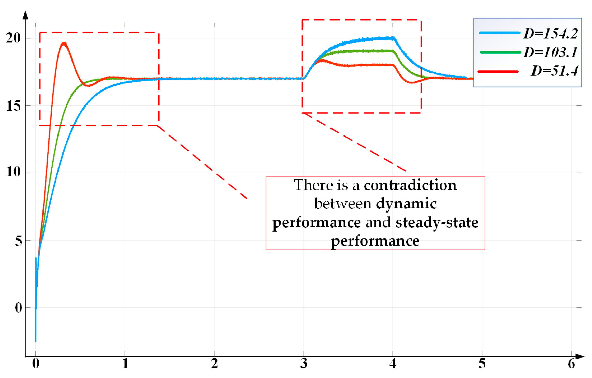
- The impact of the damping coefficient on active frequency modulation is analyzed, revealing that increasing the coefficient reduces low-frequency oscillations but induces active steady-state errors. This part is located in Section 3 of the article.
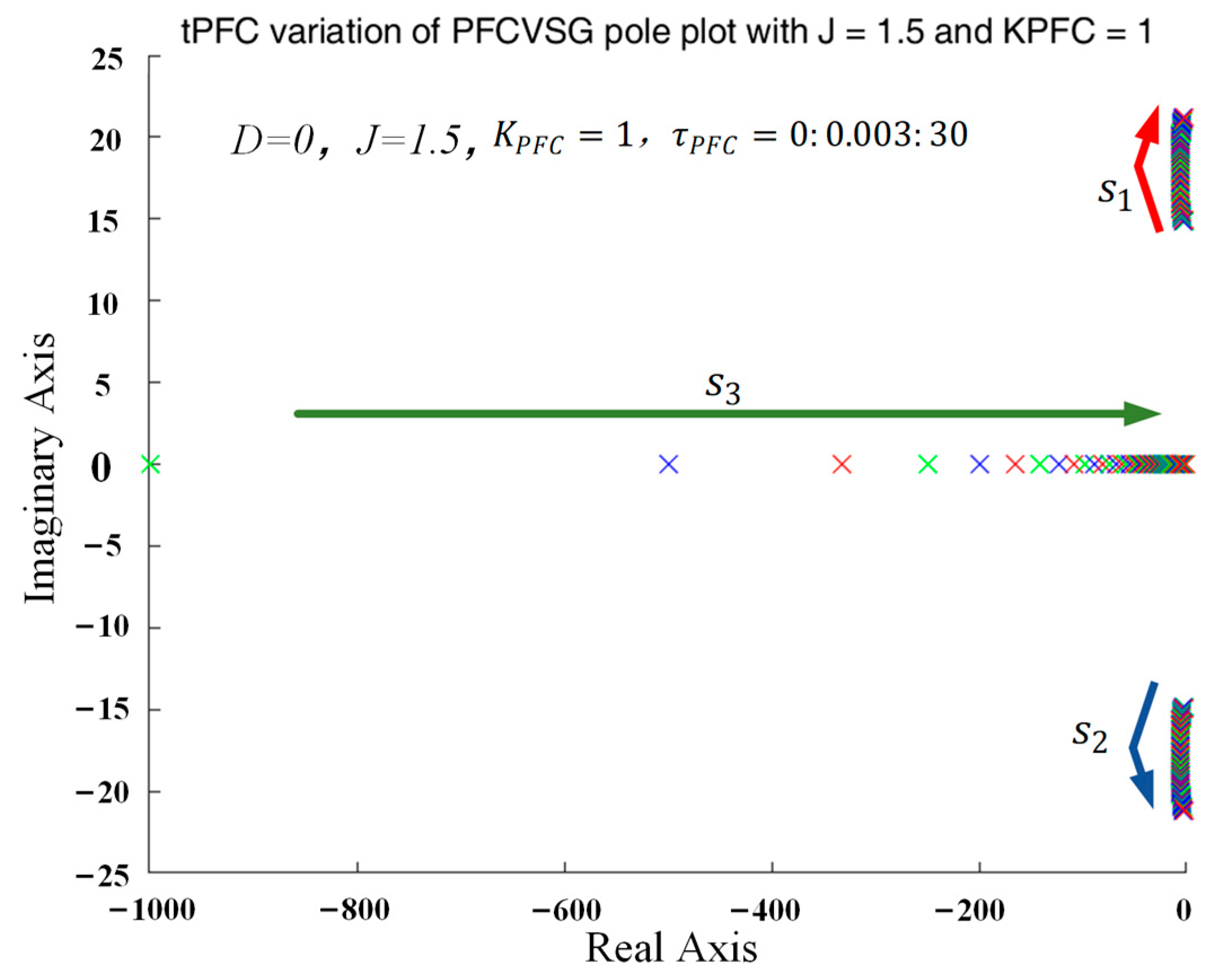
- PFFCVSG is systematically investigated using a small-signal model. The effects of the compensation coefficient and lag time constant are analyzed, parameter setting methods are provided, and the frequency overshoot issue is highlighted. This part is located in Section 4 of the article.
- Identifying weakened inertia as the cause of frequency overshoot in PFFCVSG, an active feedforward compensation strategy based on adaptive virtual inertia (PFFCVSG_AJ) is proposed. The article presents the variation range of the adaptive virtual inertia constant, details its control method, and presents the theoretical basis for the method to adjust in the face of power grid frequency changes and sudden load mutations. This part is located in Section 5 of the article.
2. Analysis of the Control Principle and Small-Signal Model of the VSG
2.1. Basic Control Principle of VSG
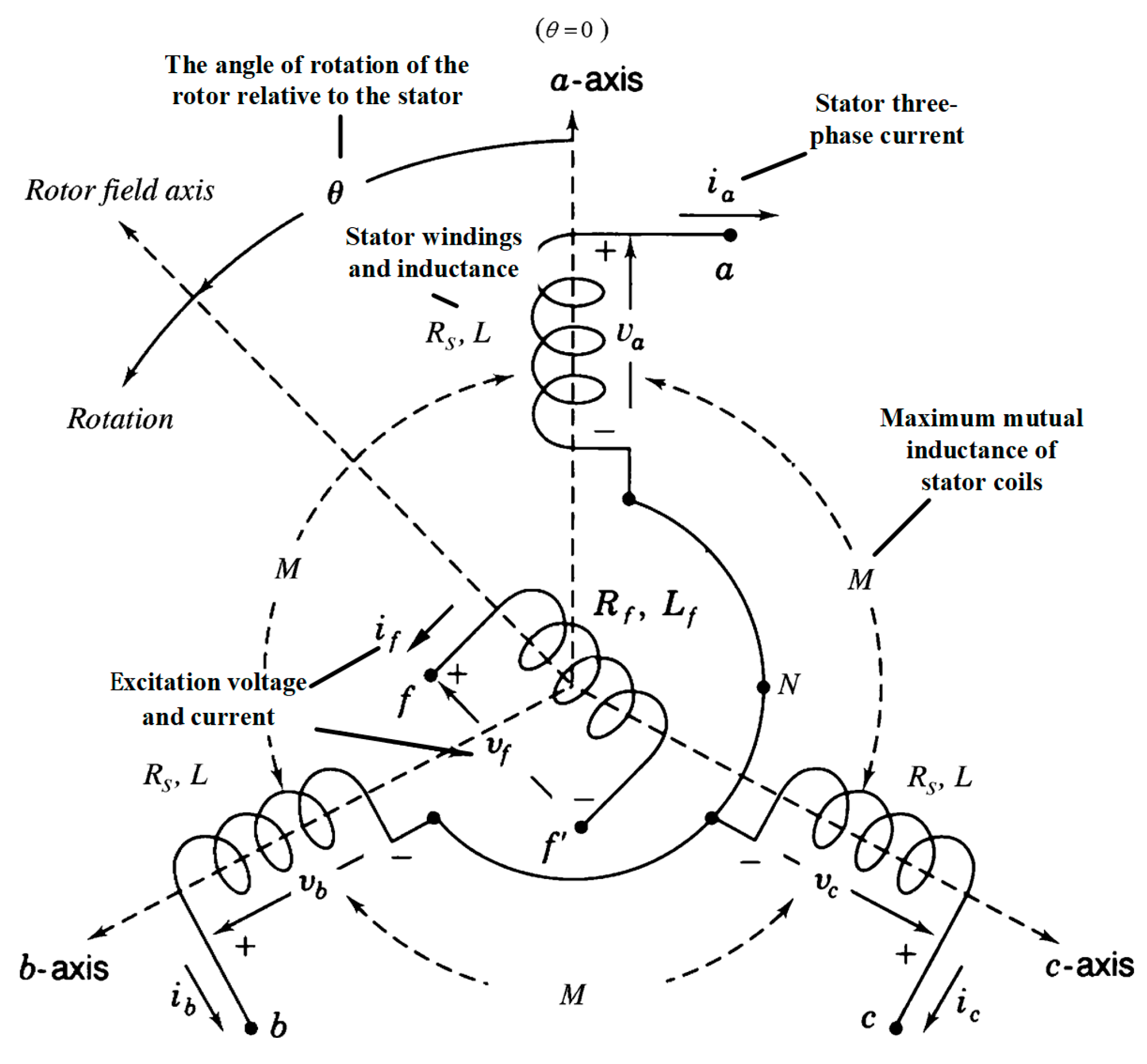
2.1.1. Synchronous Machine and Virtual Synchronous Generator
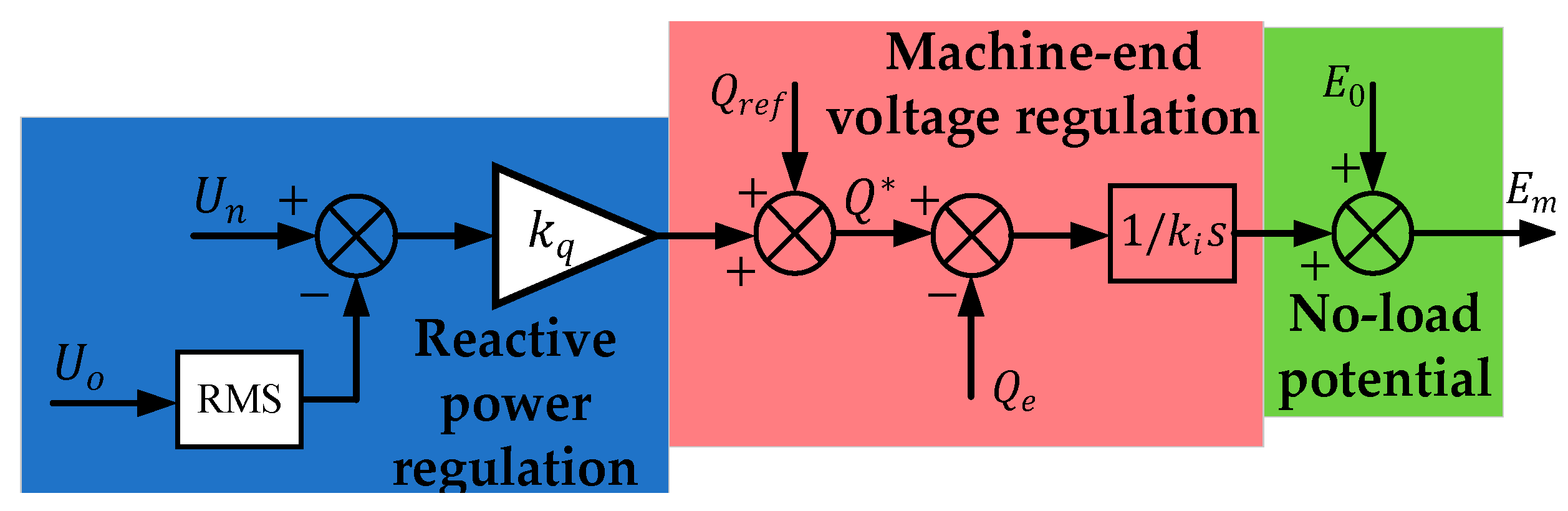
2.1.2. Active Power–Frequency Control and Reactive Power–Voltage Control
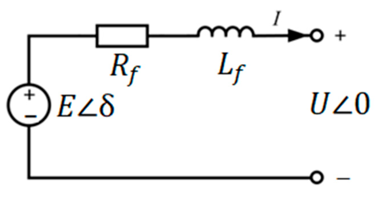
2.1.3. Virtual Impedance Control Structure
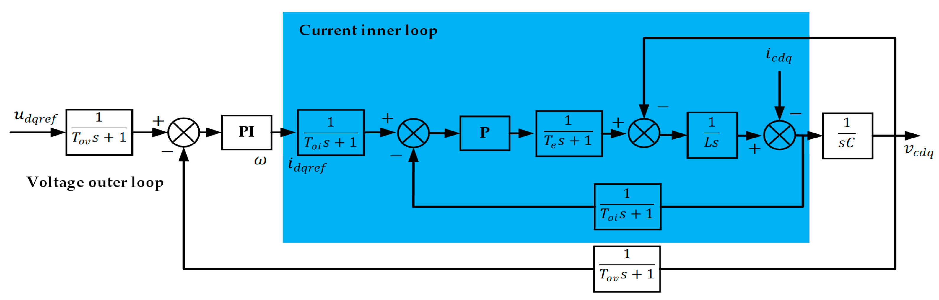
2.1.4. The -Based Dual-Loop Control for Voltage and Current
2.2. Analysis of VSG Control Small-Signal Model
3. Problems of Active Power, Low-Frequency Oscillation and Steady-State Error of VSG
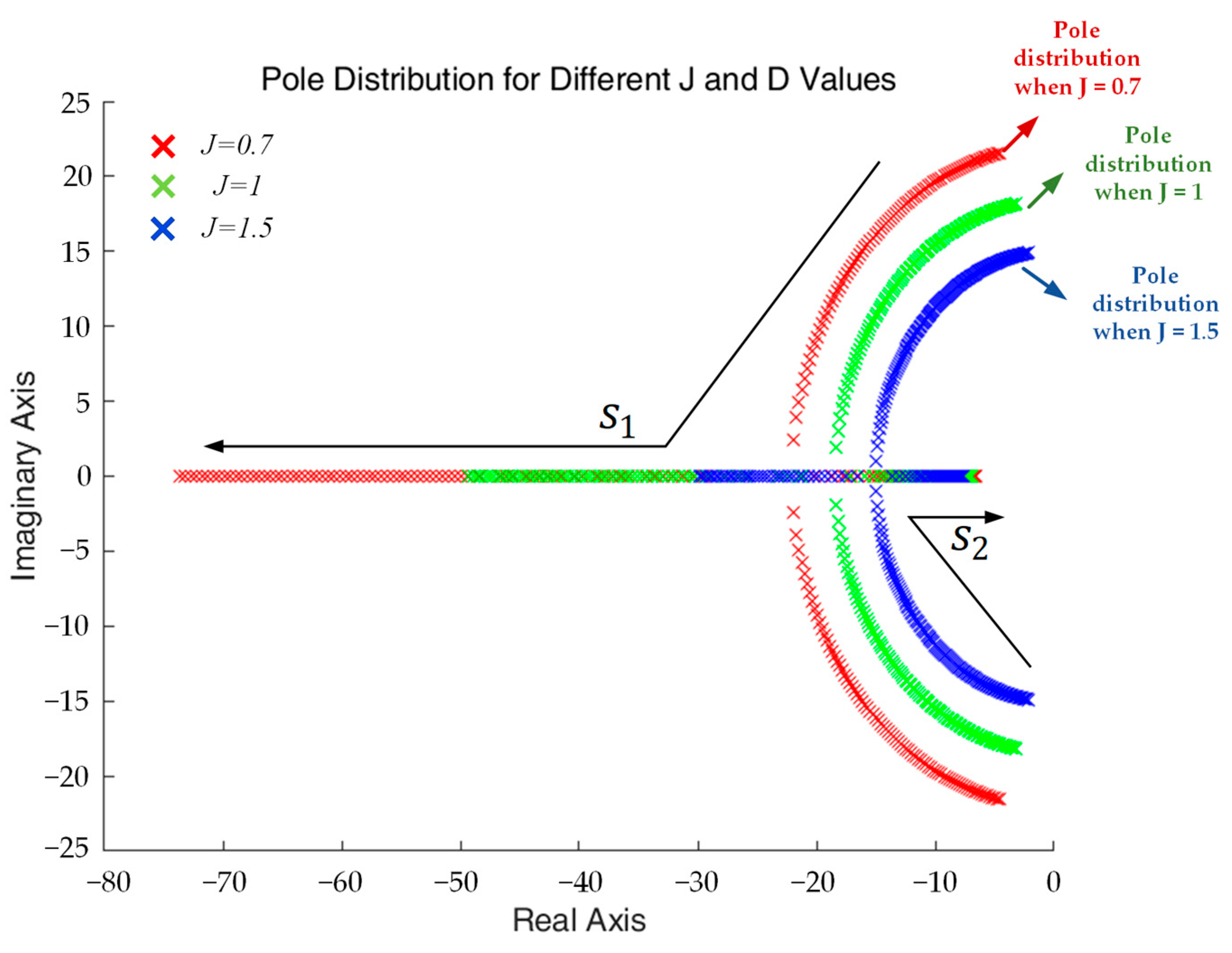
3.1. Influence of Virtual Damping Parameters ()
3.2. Low-Frequency Oscillation and Steady-State Error Problems of VSG
4. Active Power Differential Feedforward Compensation Strategy
- It disrupts the damping feedback mechanism of VSG in the theoretical model;
- It causes sustained oscillations in system stability;
- It exacerbates frequency and power fluctuations in the dynamic response.
5. Adaptive Virtual Inertia Adjustment Method Based on PFFCVSG
5.1. Analysis of Adaptive Virtual Inertia Constant
5.2. Coordinated Control Method Based on PFFCVSG_AJ
- In interval ①, RoCoF first increases and then decreases to 0. This is because when the power increases from to , the input power of the system increases, resulting in an acceleration trend of the angular velocity , which leads to an increase in RoCoF. As the system gradually adjusts, RoCoF gradually decreases to 0. In this interval, , the actual angular velocity of the system is greater than the rated angular velocity , the system is in an accelerating state, and the frequency increases. At this time, it is necessary to appropriately increase to suppress the excessive frequency change.
- In interval ②, the power continues to change from , first increases and then gradually decreases, and at this time, and is in a decelerating state. In this interval, and the actual angular velocity is still greater than the rated angular velocity but is gradually decreasing. At this time, can be appropriately reduced because the system needs to adjust the frequency more quickly. A smaller can reduce the inertia of the system within an appropriate range to accelerate the response speed and make return to the rated angular velocity more quickly.
- In interval ③, the power decreases from to ; at this time and deviates from in the reverse direction. At this time and the frequency gradually decreases. In this interval, it is necessary to increase . A larger can increase the inertia of the system, making the system’s response to frequency changes slower and suppressing the reverse deviation trend.
- In interval ④, the power decreases from to ; at this time and starts to accelerate and recover in the positive direction. In this interval, and gradually increases and approaches . At this time, it is necessary to reduce within the specified range, appropriately reduce the inertia of the system, and make respond to power changes more quickly and reduce the time to return to .
- For the parameter, its role is to avoid the frequent charging and discharging of devices caused by minor frequency fluctuations. It is set according to the allowable frequency deviation range of the system. As described in Section 5.1, within a small-system-capacity range, the frequency deviation is ±0.5 Hz; thus is set to 0.5.
- The setting of the parameter is combined with the dynamic response characteristics of the system, and needs to be determined by the minimum rate of frequency change that can trigger the condition. According to the content in [23], it is determined that the maximum rate of frequency change in the system is ; thus can be set as a safety margin close to this value ().
5.3. Performance Analysis of PFFCVSG_AJ Under External Disturbances
5.3.1. Theoretical Analysis Under Grid Frequency Disturbance
5.3.2. Theoretical Analysis Under Load Mutation
- Load mutation identification: When the load changes abruptly, the output power of the system will change rapidly. By sensing the power change rate , the system can quickly sense the load change and quickly trigger the adjustment of the virtual inertia .
- Virtual inertia transient increases: When the load change is perceived, the can be quickly increased, thereby extending the window of power balance, so that the frequency and voltage do not fluctuate greatly.
6. Simulation Results
6.1. Comparative Simulation Verification
6.2. Simulation Under the Condition of Changing the Active Power Command
6.3. Performance of PFFCVSG_AJ Under Different
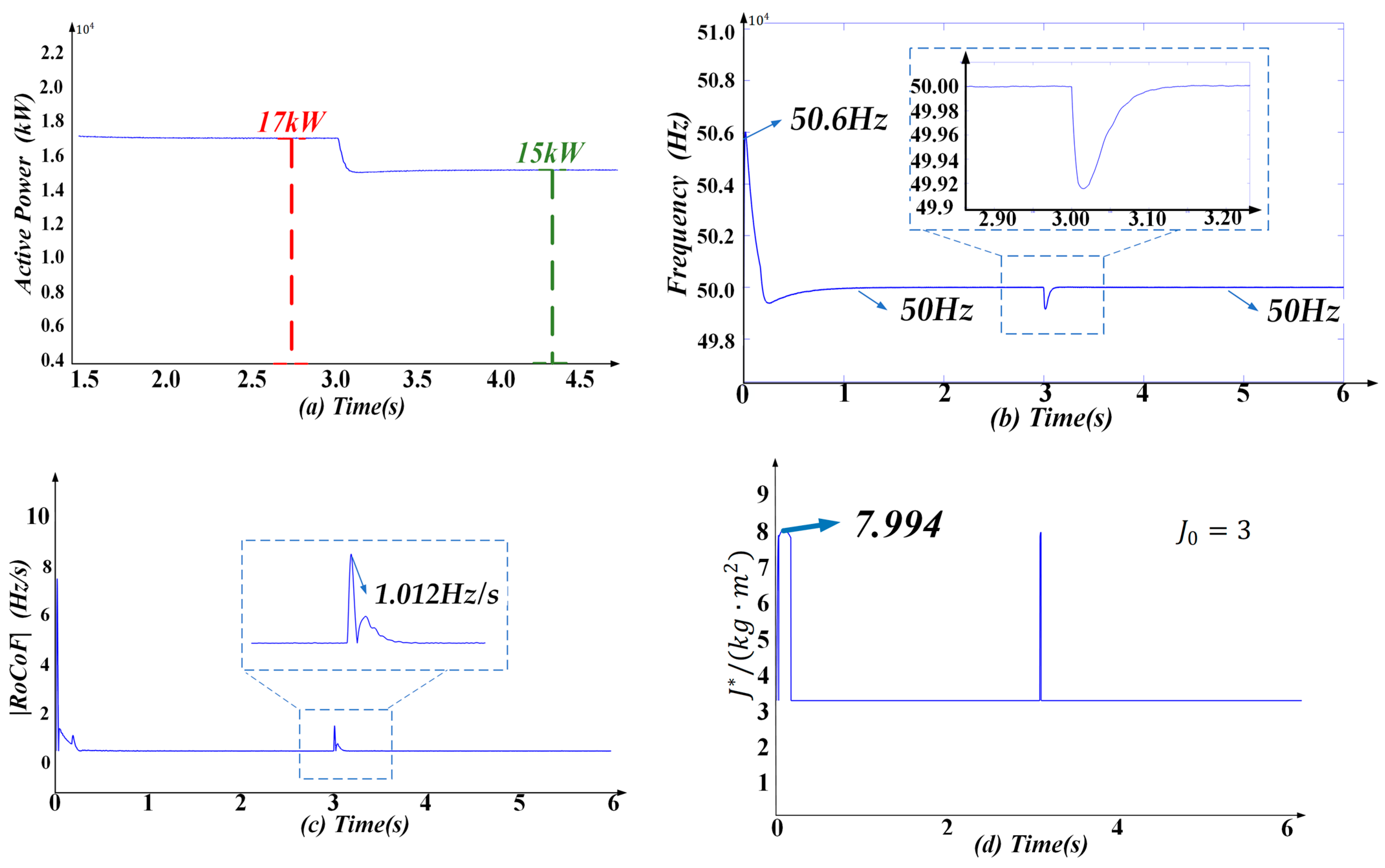
- For different values of , the mutation problem of the virtual inertia constant is well suppressed, and the change range always meets the requirement range of . The larger the , the smoother the change of , which also verifies the previous analysis of the influence of on the system.
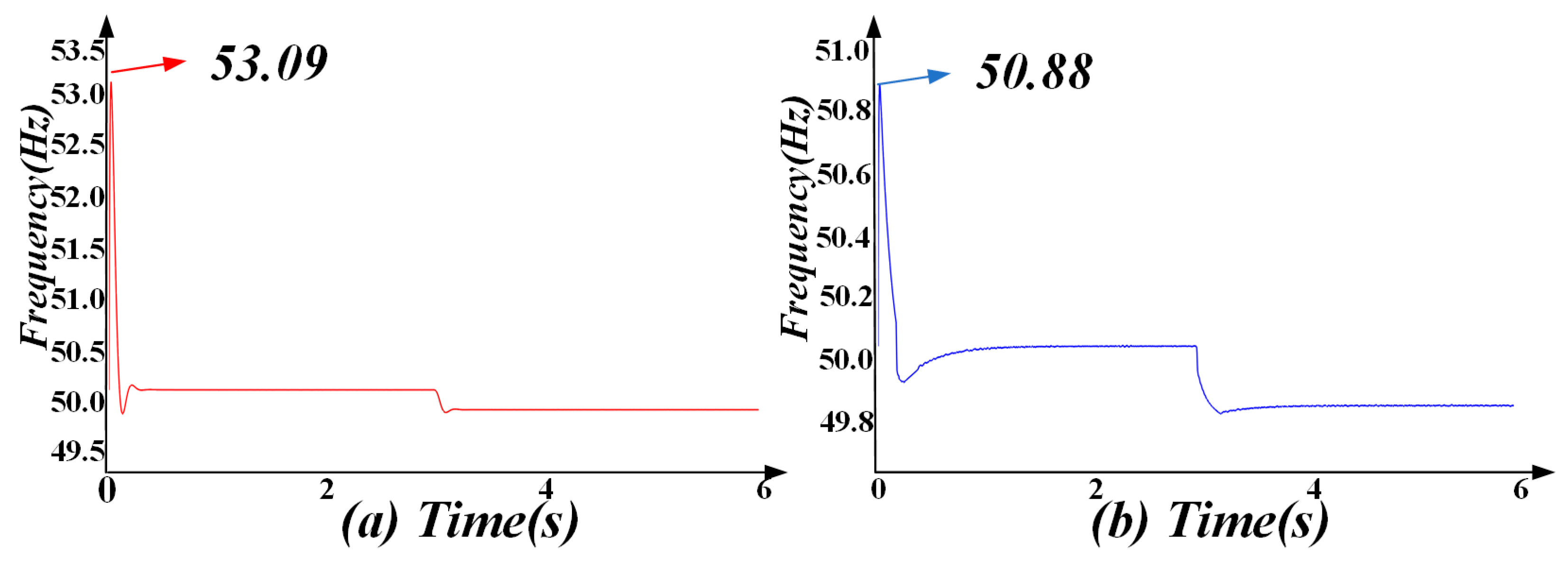
- The frequency mutation problem is well solved. The RFD of the system is basically in the range of 50.5–51 Hz, and as increases, the RFD value is smaller.
- The active power oscillation changes at 3 s due to the change in the grid frequency. Following the completion of frequency tracking, the active power can be stabilized near 17.2 kW. For different values of , the steady-state values of the active power exhibit minimal difference, which verifies that PFFCVSG_AJ only affects the dynamic performance of the system during the tracking process and does not change the steady-state value of the system, thus effectively solving the problem of the active power steady-state error.
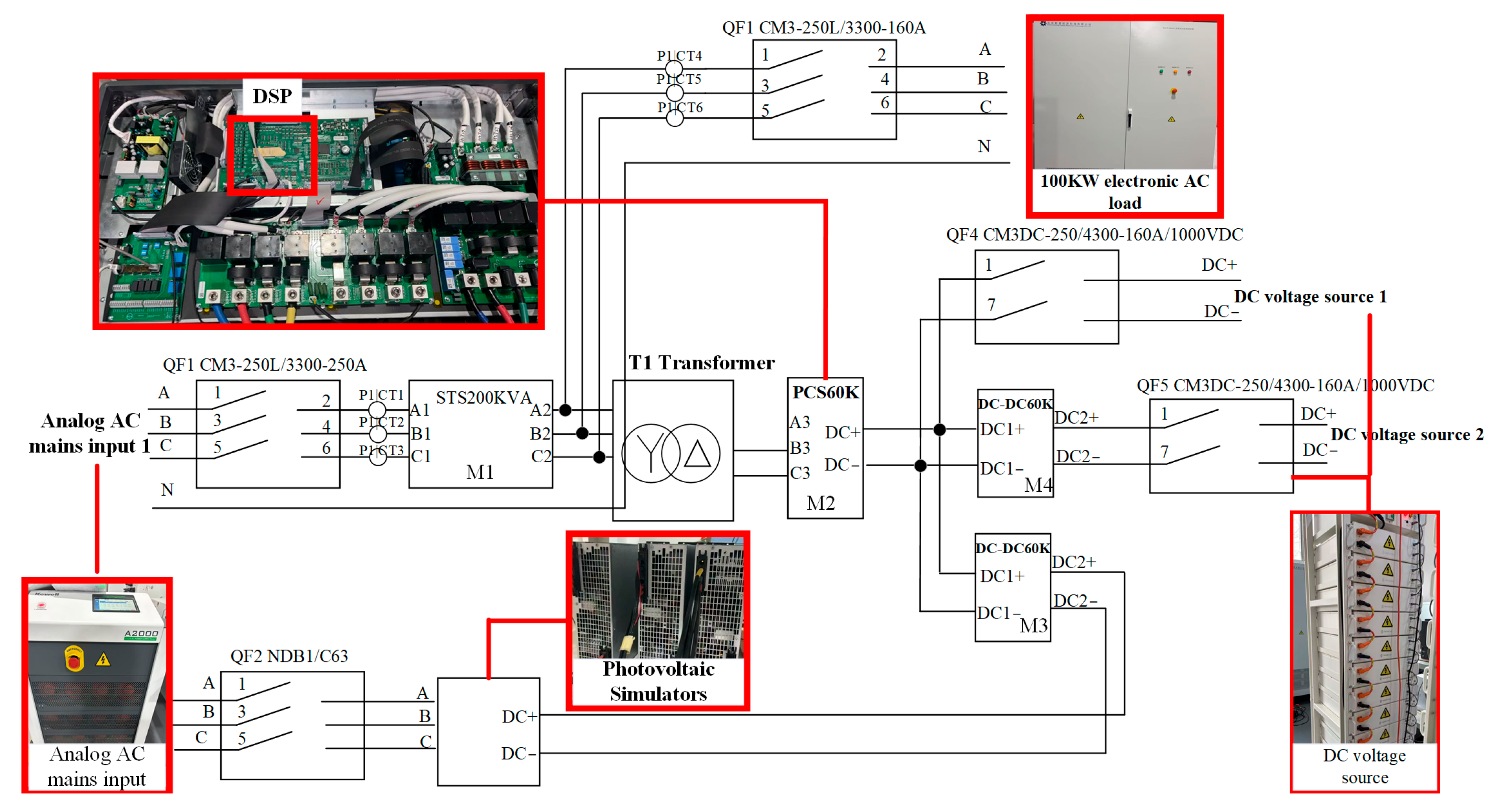
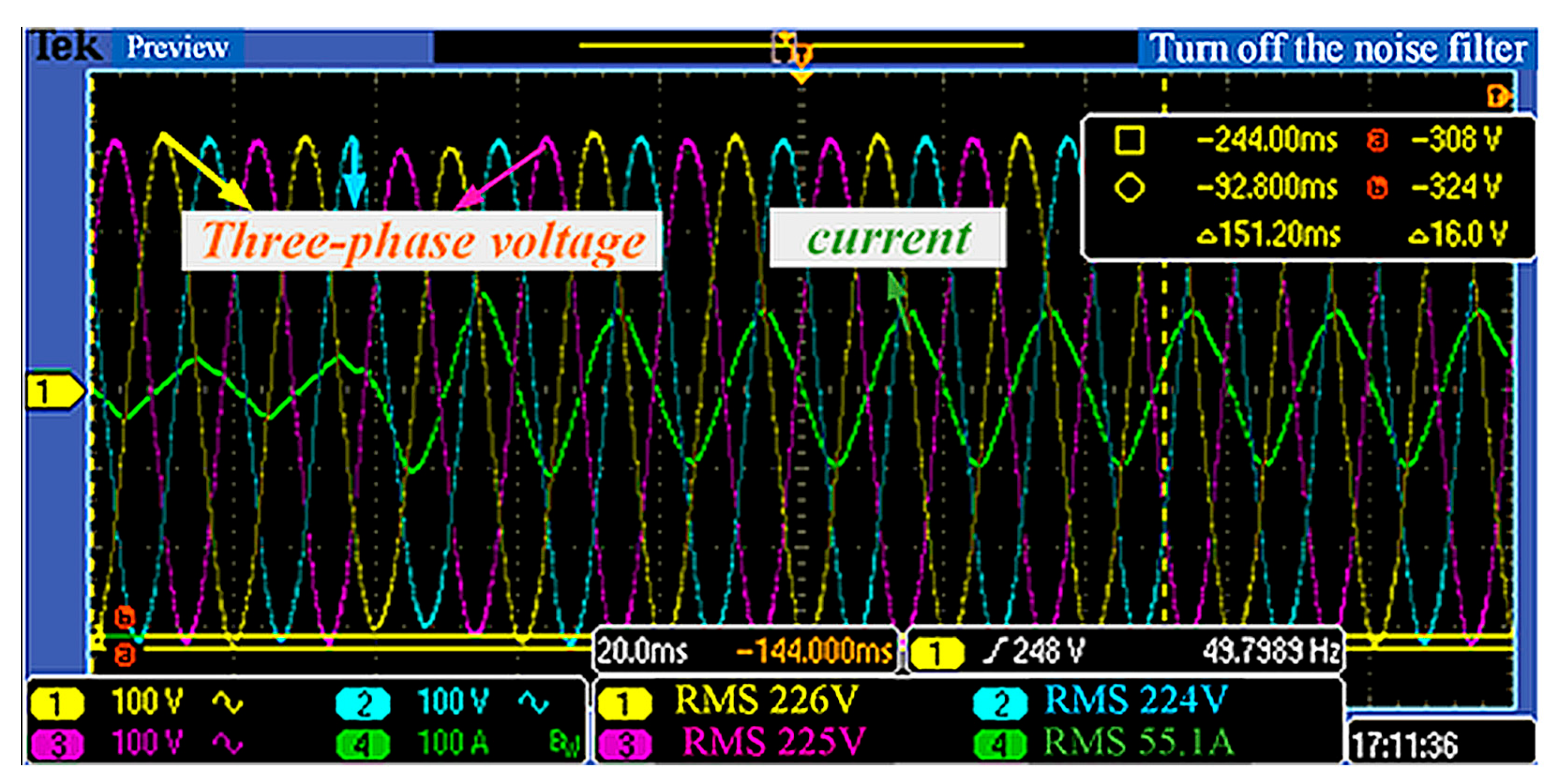
7. Experimental Results
8. Discussion and Conclusions
Author Contributions
Funding
Data Availability Statement
Conflicts of Interest
Abbreviations
| VSG | Virtual synchronous generator |
| SG | Synchronous generator |
| PFFCVSG | Active power differential feedforward compensation strategy |
| PFFCVSG_AJ | Adaptive virtual inertia method based on PFFCVSG |
| RoCoF | Rate of change in frequency |
| SSOP | Steady-state operating point |
References
- Lyu, Z.P.; Sheng, W.X.; Zhong, Q.C.; Liu, H.T.; Zeng, Z.; Yang, L.; Liu, L. Virtual synchronous generator its application in microgrid. Chin. J. Electr. Eng. 2014, 34, 2591–2603. [Google Scholar] [CrossRef]
- Yan, L.Q.; Zhao, Z.; Ullah, Z.; Deng, X.W.; Zhang, Y.Y.; Shah, W.A. Optimization of optical storage VSG control strategy considering active power deviation and virtual inertia damping parameters. Ain Shams Eng. J. 2024, 15, 103131. [Google Scholar] [CrossRef]
- Lu, S.; Zhu, Y.; Dong, L.; Na, G.; Hao, Y.; Zhang, G.; Zhang, W.; Cheng, S.; Yang, J.; Sui, Y. Small-Signal Stability Research of Grid-Connected Virtual Synchronous Generators. Energies 2022, 15, 7158. [Google Scholar] [CrossRef]
- Qi, X.; Zheng, J. VSG Control for Cascaded Three-Phase Bridge Based Battery Inverter. World Electr. Veh. J. 2023, 14, 203. [Google Scholar] [CrossRef]
- Shi, R.L.; Wang, B.; Huang, J.; Wang, G.B.; Lan, C.H. Analysis and Improvement Strategy of Grid-Connected Damping Characteristics of Energy Storage Virtual Synchronous Machine. Acta Energiae Solaris Sin. 2023, 44, 30–38. [Google Scholar] [CrossRef]
- Shi, R.L.; Lan, C.H.; Dong, Z.; Yu, Y.N.; Zhong, Z.X. An Active Power Oscillation Damping Strategy for Grid-Forming Energy Storage Virtual Synchronous Generator (VSG) Based on Energy Reconfiguration. Acta Energiae Solaris Sin. 2025, 46, 300–308. [Google Scholar] [CrossRef]
- Zhou, N.G.; Xie, X.T.; Ma, J.J.; Yu, H.F.; Li, Y.; Xie, Y.Z. Adaptive Virtual Inertia-Damping Control for Wind Farm-Equipped Energy Storage. J. Electr. Sci. Technol. China 2024, 39, 150–158. [Google Scholar] [CrossRef]
- Dong, S.; Chen, Y.C. Adjusting synchronverter dynamic response speed via damping correction loop. IEEE Trans. Energy Convers. 2017, 32, 608–619. [Google Scholar] [CrossRef]
- Li, C.; Yang, Y.; Mijatovic, N.; Dragicevic, T. Frequency stability assessment of grid-forming VSG in framework of MPME with feedforward decoupling control strategy. IEEE Trans. Ind. Electron. 2022, 69, 6903–6913. [Google Scholar] [CrossRef]
- Lan, C.H.; Shi, R.L.; Wang, G.B.; Zhou, Q.F.; Liu, W.S. Optimization Strategy for Grid-Connected Active Power Response of Energy Storage VSG Based on Frequency Feedforward Compensation. Acta Energiae Solaris Sin. 2024, 45, 236–243. [Google Scholar] [CrossRef]
- Xiong, X.L.; Li, X.; Luo, B.; Huang, M.; Zhao, C.; Blaabjerg, F. An Additional Damping Torque Method for Low-Frequency Stability Enhancement of Virtual Synchronous Generators. IEEE Trans. Power Electron. 2024, 39, 15858–15869. [Google Scholar] [CrossRef]
- Chen, S.M.; Sun, Y.; Han, H.; Luo, Z.Z.; Shi, G.Z.; Yuan, L.; Guerrero, J.M. Active power oscillation suppression and dynamic performance improvement for multi-VSG grids based on consensus control via COI frequency. Int. J. Electr. Power Energy Syst. 2023, 147, 108796. [Google Scholar] [CrossRef]
- Ling, S.; Liu, R.H.; Zhang, C.Y.; Wang, X.D.; Yang, X.W. Subsynchronous oscillation suppression strategy of virtual synchronous generator based on dynamic inertia damping coefficient. China South. Power Grid Technol. 2025, 1–10, in press. Available online: https://nfdwjs.csg.cn/gateway-web/en/debutDetail.html?serialNum=20241220001 (accessed on 14 June 2025).
- Lan, Z.; Long, Y.; Zeng, J.H.; Tu, C.M.; Xiao, F.; Guo, Q. Transient Power Oscillation Suppression Strategy of Virtual Synchronous Generator Considering Overshoot. Autom. Electr. Power Syst. 2022, 46, 131–141. [Google Scholar] [CrossRef]
- Zhuo, Q.; Liu, W.; Xu, Z.; Zhang, H.; Zhai, Y.; Yang, L. Active Power-Frequency Oscillation Suppression Strategy for Parallel VSG Grid-Connected Power System. In Proceedings of the 2024 10th International Conference on Power Electronics Systems and Applications (PESA), Hong Kong, China, 5–7 June 2024. [Google Scholar] [CrossRef]
- Bal, G. Performance Analysis of Field-Orientation Controlled Induction Motor with Parameter Adaptation; University of Strathclyde: Glasgow, UK, 1993. [Google Scholar]
- Ban, G.; Xu, Y.; Guo, D.; Zhou, W.; Zheng, H.; Yuan, X. Research on adaptive VSG control strategy based on inertia and damping. In Proceedings of the 2021 IEEE International Conference on Sustainable Power and Energy (iSPEC), Nanjing, China, 23–25 December 2021. [Google Scholar] [CrossRef]
- Jain, A.; Pathak, M.K.; Padhy, N.P. Conjoint Enhancement of VSG Dynamic Output Responses by Disturbance-Oriented Adaptive Parameters. IEEE Trans. Ind. Inform. 2024, 20, 2079–2096. [Google Scholar] [CrossRef]
- Zhang, C.; Yang, Y.; Miao, H.; Yuan, X. An improved adaptive inertia and damping control strategy for virtual synchronous generator. In Proceedings of the 2018 13th IEEE Conference on Industrial Electronics and Applications (ICIEA), Wuhan, China, 31 May–2 June 2018. [Google Scholar] [CrossRef]
- Yan, L.Q.; Deng, X.W.; Zhao, Z.; Zhang, Y.Y.; Yuan, Y.; Peng, P.P. VSG Power Decoupling Control Strategy Based on Adaptive Feedforward Compensation. Power Syst. Prot. Control 2024, 52, 64–73. [Google Scholar] [CrossRef]
- Chen, S.; Sun, Y.; Han, H.; Shi, G.; Guan, Y.; Guerrero, J.M. Dynamic Frequency Performance Analysis and Improvement for Parallel VSG Systems Considering Virtual Inertia and Damping Coefficient. IEEE J. Emerg. Sel. Top. Power Electron. 2023, 11, 478–489. [Google Scholar] [CrossRef]
- Zhong, Q.C.; Weiss, G. Synchronverters: Inverters That Mimic Synchronous Generators. IEEE Trans. Ind. Electron. 2011, 58, 1259–1267. [Google Scholar] [CrossRef]
- Liu, H.; Gao, S.A.; Sun, D.W.; Song, P.; Wang, X.S.; Cheng, X.K. Small-Signal Stability Analysis of Photovoltaic Virtual Synchronous Generator Grid-Connected. Acta Energiae Solaris Sin. 2021, 42, 417–424. [Google Scholar] [CrossRef]
- Zhang, X. Advanced Power Electronics Technology; China Machine Press: Beijing, China, 2011. [Google Scholar]
- Cheema, K.M. A comprehensive review of virtual synchronous generator. Int. J. Electr. Power Energy Syst. 2020, 120, 106006. [Google Scholar] [CrossRef]
- GB/T 15945-2008; Power Quality-Power System Frequency Deviation. Standards Press of China: Beijing, China, 2008.
- Wang, L.; Ren, J.; Huang, G.; Xie, L.; Feng, C.; Zhang, Y. Identifying the Largest RoCoF and Its Implications. IEEE Trans. Power Syst. 2025, 40, 1164–1167. [Google Scholar] [CrossRef]
- Zheng, C.; Sun, H.D.; Zhang, H.Y.; Du, Y. Transient power angle stability emergency control of VSG single-machine grid-connected system based on network disturbance response. Chin. J. Electr. Eng. 2025, 1–13, in press. [Google Scholar]
- Zhang, C.W.; Shi, Y.F.; Zhan, X.; Liu, Z.H.; Sun, L. TMD control system based on motion form transformation using rotational inertia virtual translational inertia mass. Vib. Eng. J. 2024, 37, 1377–1385. [Google Scholar]


| Parameters | Value | Parameters | Value |
|---|---|---|---|
| Rated Voltage/V | 380 | 640.146 | |
| Rated Frequency/Hz | 50 | 96.774 | |
| /H | 3 × 10⁻³ | 0 | |
| /F | 35 × 10−6 | 0.4 | |
| Line Impedance X | 0.06 + j(1.35 × 10⁻³) Ω | 0.5 | |
| 1.95 | −0.01 |
| Indexes | Basic VSG Method | PFFCVSG Method | PFFCVSG_AJ Method |
|---|---|---|---|
| Active steady-state power value | W | W | W |
| Damping situation | Critical damping | Underdamping | Overdamping |
| Steady-state error | W | 0 W | 0 W |
| Overshoot condition | Exists | Exists | Exists but is smaller than the traditional VSG |
| Indexes | Basic VSG Method | PFFCVSG Method | PFFCVSG_AJ Method |
|---|---|---|---|
| 0.55 Hz | 3.09 Hz | 0.88 Hz | |
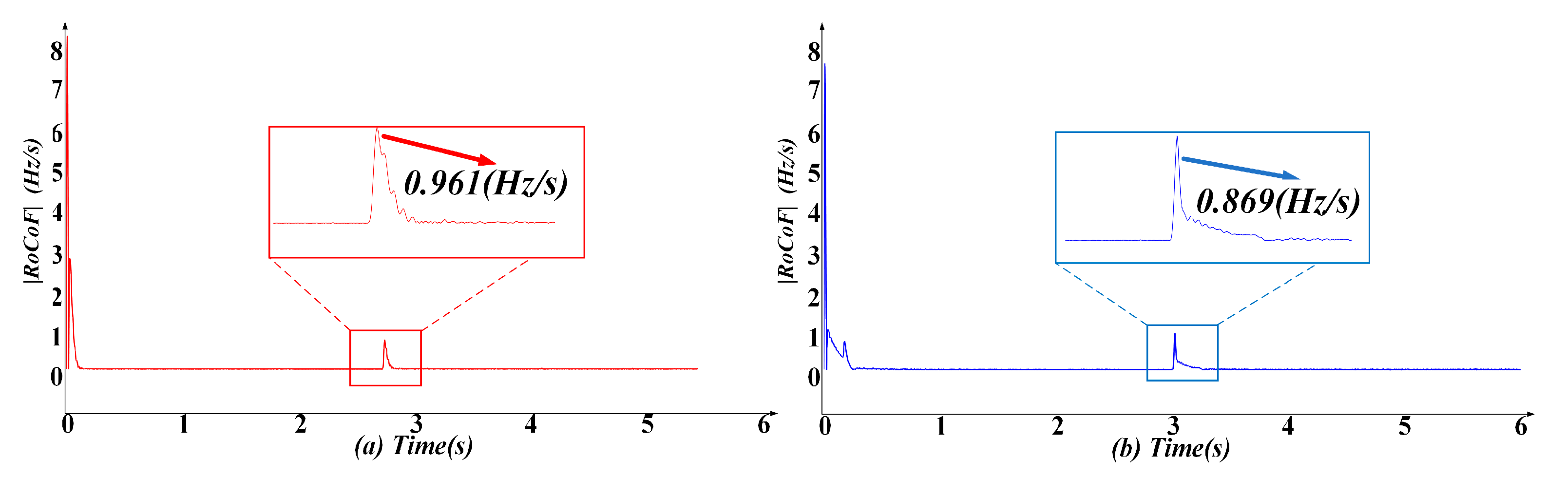
| 1.21 Hz/s | 0.961 Hz/s | 0.869 Hz/s | |
| dynamic performance stability time | 1.91 s | 1.03 s | 1.02 s |
| Active Steady-State Power Value | ||
|---|---|---|
| 0.6 Hz | 1.012 Hz/s | 17–15 kW |
| Active Steady-State Power Value | |||
|---|---|---|---|
| 8.487 | 50.88 Hz | 17.2 kW | |
| 7.998 | 50.72 Hz | 17.2 kW | |
| 7.994 | 50.61 Hz | 17.1 kW |
Disclaimer/Publisher’s Note: The statements, opinions and data contained in all publications are solely those of the individual author(s) and contributor(s) and not of MDPI and/or the editor(s). MDPI and/or the editor(s) disclaim responsibility for any injury to people or property resulting from any ideas, methods, instructions or products referred to in the content. |
© 2025 by the authors. Licensee MDPI, Basel, Switzerland. This article is an open access article distributed under the terms and conditions of the Creative Commons Attribution (CC BY) license (https://creativecommons.org/licenses/by/4.0/).
Share and Cite
Cao, X.; Zhang, R.; Li, J.; Ji, L.; Wei, X.; Geng, J.; Li, B. Analysis of Grid-Connected Damping Characteristics of Virtual Synchronous Generator and Improvement Strategies. Electronics 2025, 14, 2501. https://doi.org/10.3390/electronics14122501
Cao X, Zhang R, Li J, Ji L, Wei X, Geng J, Li B. Analysis of Grid-Connected Damping Characteristics of Virtual Synchronous Generator and Improvement Strategies. Electronics. 2025; 14(12):2501. https://doi.org/10.3390/electronics14122501
Chicago/Turabian StyleCao, Xudong, Ruogu Zhang, Jun Li, Li Ji, Xueliang Wei, Jile Geng, and Bowen Li. 2025. "Analysis of Grid-Connected Damping Characteristics of Virtual Synchronous Generator and Improvement Strategies" Electronics 14, no. 12: 2501. https://doi.org/10.3390/electronics14122501
APA StyleCao, X., Zhang, R., Li, J., Ji, L., Wei, X., Geng, J., & Li, B. (2025). Analysis of Grid-Connected Damping Characteristics of Virtual Synchronous Generator and Improvement Strategies. Electronics, 14(12), 2501. https://doi.org/10.3390/electronics14122501