
Optimizing Glioblastoma Multiforme Diagnosis: Semantic Segmentation and Survival Modeling Using MRI and Genotypic Data


Abstract
1. Introduction
- This study explores the combination of image processing techniques and deep learning models for segmenting GBM MRI images and finds that such integration can significantly improve segmentation performance.
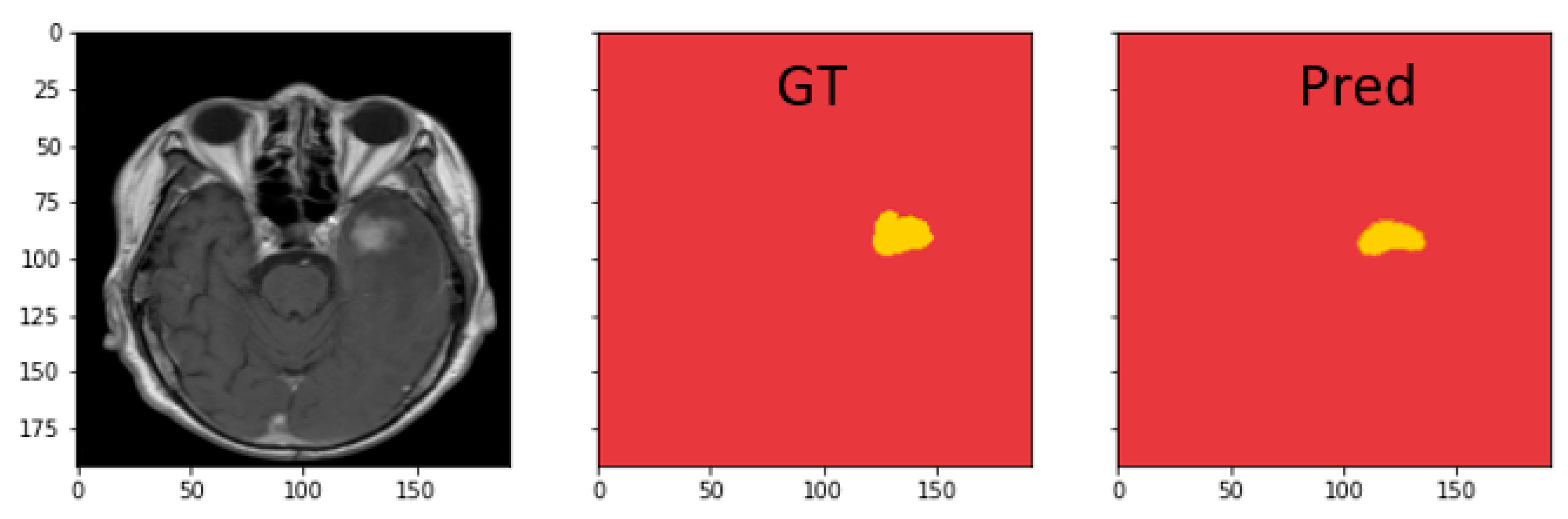
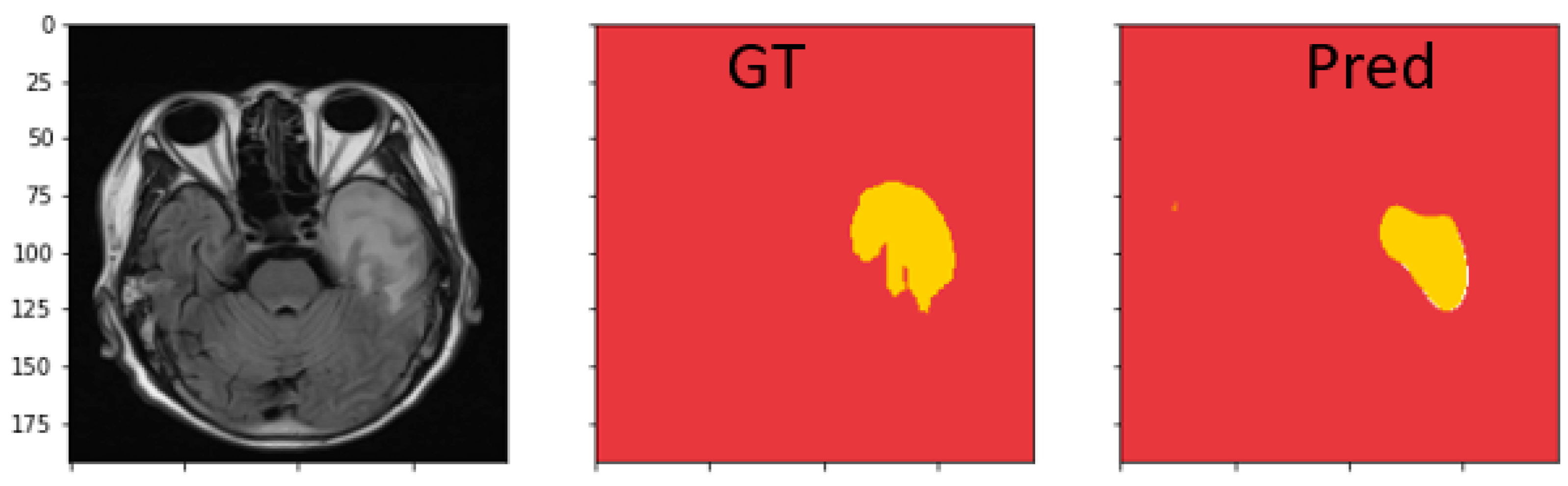
- For T1WI, the highest Dice coefficient of 0.779 is achieved when applying Intensity Normalization as preprocessing followed by the DeepLabV3+ model. For FLAIR imaging, the highest Dice coefficient of 0.801 is obtained when using GRAR preprocessing combined with the U-Net model.
- The DeepLabV3+ model shows Dice coefficient improvements of 0.156 and 0.149 on T1WI and FLAIR images, respectively, when using intensity normalization as preprocessing.
- Using gene data from GBM patients, this study predicts survival outcomes. When missing values are replaced with 1, the NB model achieves an accuracy of 0.9474.
2. Related Works
2.1. Medical Image Features
2.2. Medical Image Segmentation
2.3. Deep Learning for Brain Tumor Image Segmentation
2.4. Digital Image Processing
3. Materials and Methods
3.1. Datasets
- VEGF (vascular endothelial growth factor) [50] primarily binds to receptors on vascular endothelial cells (VEGF receptors, VEGFR), thereby promoting tumor growth.
- IDH (isocitrate dehydrogenase) [51] refers to a group of enzymes divided into IDH1 and IDH2. Mutations in IDH are associated with the development of glioblastoma.
- hTERT (human telomerase reverse transcriptase) [52] is commonly considered an oncogene when mutated.
- MGMT (O6-methylguanine-DNA methyltransferase) [53] is a DNA repair gene. MGMT is often involved in promoter methylation, which can interfere with the DNA repair process.
- p53 [54] refers to a family of homologous proteins known as tumor suppressors.
- p21 [55], also known as CDKN1A (cyclin-dependent kinase inhibitor 1A), is a tumor suppressor protein involved in regulating the cell cycle.
3.2. Screening and Labeling of MRI Images
3.3. Screening and Handling Missing Values of Genetic Data
3.4. Image Processing
3.4.1. AHE
3.4.2. Intensity Normalization
3.4.3. BFC
3.4.4. GRAR
3.5. Semantic Segmentation
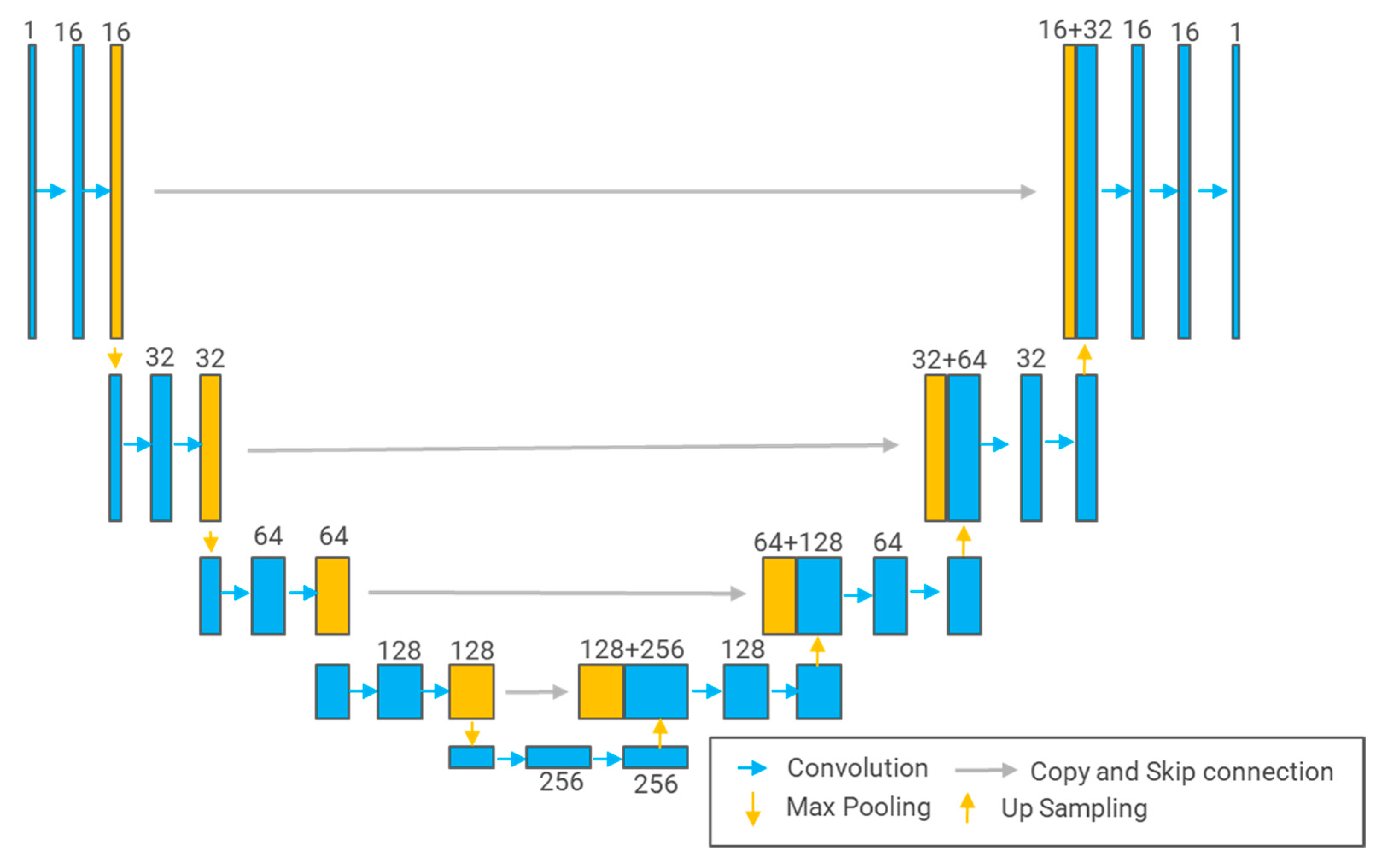
3.5.1. U-Net
3.5.2. U-Net++
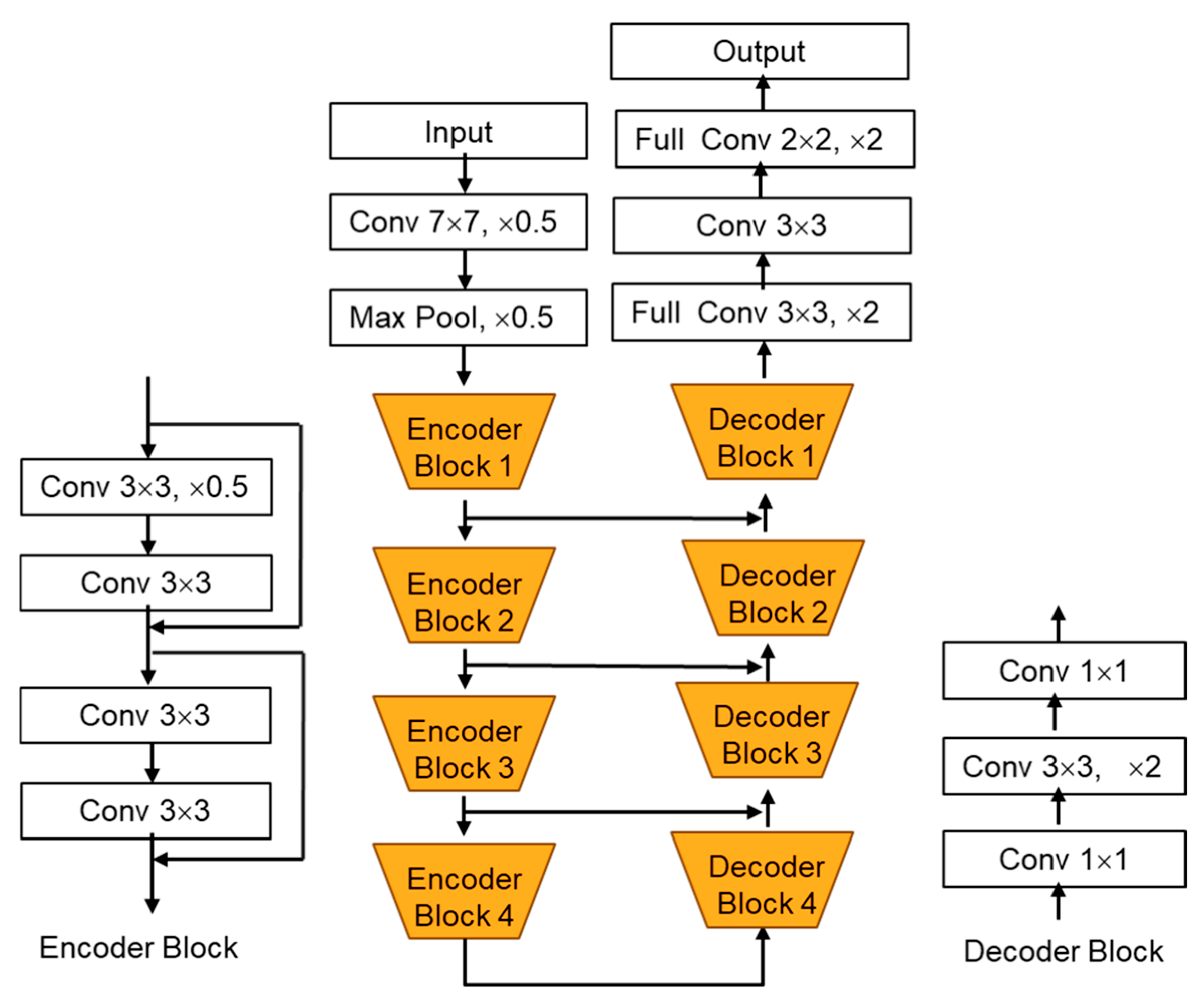
3.5.3. DeepLabV3+
3.5.4. LinkNet
4. Results and Discussion
4.1. The Results of Screening and Labeling of MRI Images
4.2. The Results of Screening and Handling Missing Values of Genetic Data
4.3. Image Processing Results
4.4. Semantic Segmentation Results
4.4.1. Comparison Results of Model Performance for T1WI Sequence
4.4.2. Comparison Results of Model Performance for FLAIR Sequence
4.4.3. Discussion on MRI Semantic Segmentation
4.5. Survival Classification Results
5. Conclusions
Author Contributions
Funding
Institutional Review Board Statement
Informed Consent Statement
Data Availability Statement
Acknowledgments
Conflicts of Interest
References
- Jiang, H.; Wang, X.; Chen, X.; Zhang, S.; Ren, Q.; Li, M.; Ren, X.; Lin, S.; Cui, Y. Unraveling the heterogeneity of WHO grade 4 gliomas: Insights from clinical, imaging, and molecular characterization. Discov. Oncol. 2025, 16, 111. [Google Scholar] [CrossRef] [PubMed]
- Grochans, S.; Cybulska, A.M.; Simińska, D.; Korbecki, J.; Kojder, K.; Chlubek, D.; Baranowska-Bosiacka, I. Epidemiology of glioblastoma multiforme–literature review. Cancers 2022, 14, 2412. [Google Scholar] [CrossRef]
- Koshy, M.; Villano, J.L.; Dolecek, T.A.; Howard, A.; Mahmood, U.; Chmura, S.J.; Weichselbaum, R.R.; McCarthy, B.J. Improved survival time trends for glioblastoma using the SEER 17 population-based registries. J. Neuro-Oncol. 2012, 107, 207–212. [Google Scholar] [CrossRef]
- Sabouri, M.; Dogonchi, A.F.; Shafiei, M.; Tehrani, D.S. Survival rate of patient with glioblastoma: A population-based study. Egypt. J. Neurosurg. 2024, 39, 42. [Google Scholar] [CrossRef]
- Wang, Y.; Xu, J.; Guan, Y.; Ahmad, F.; Mahmood, T.; Rehman, A. MSegNet: A multi-view coupled cross-modal attention model for enhanced MRI brain tumor segmentation. Int. J. Comput. Intell. Syst. 2025, 18, 63. [Google Scholar] [CrossRef]
- Shukla, G.; Alexander, G.S.; Bakas, S.; Nikam, R.; Talekar, K.; Palmer, J.D.; Shi, W. Advanced magnetic resonance imaging in glioblastoma: A review. Chin. Clin. Oncol. 2017, 6, 40. [Google Scholar] [CrossRef] [PubMed]
- Visser, M.; Müller, D.M.J.; Van Duijn, R.J.M.; Smits, M.; Verburg, N.; Hendriks, E.J.; de Munck, J.C. Inter-rater agreement in glioma segmentations on longitudinal MRI. NeuroImage Clin. 2019, 22, 101727. [Google Scholar] [CrossRef]
- Padmapriya, T.; Sriramakrishnan, P.; Kalaiselvi, T.; Somasundaram, K. Advancements of MRI-based brain tumor segmentation from traditional to recent trends: A review. Curr. Med. Imaging Rev. 2022, 18, 1261–1275. [Google Scholar]
- Bahadure, N.B.; Ray, A.K.; Thethi, H.P. Image analysis for MRI based brain tumor detection and feature extraction using biologically inspired BWT and SVM. Int. J. Biomed. Imaging 2017, 2017, 9749108. [Google Scholar] [CrossRef]
- Krizhevsky, A.; Sutskever, I.; Hinton, G.E. ImageNet classification with deep convolutional neural networks. Comm. ACM 2017, 60, 84–90. [Google Scholar] [CrossRef]
- Ronneberger, O.; Fischer, P.; Brox, T. U-net: Convolutional networks for biomedical image segmentation. In Medical Image Computing and Computer-Assisted Intervention–MICCAI 2015, Proceedings of the 18th International Conference, Munich, Germany, 5–9 October 2015; Springer: Berlin/Heidelberg, Germany, 2015. [Google Scholar]
- Ullah, F.; Ansari, S.U.; Hanif, M.; Ayari, M.A.; Chowdhury, M.E.H.; Khandakar, A.A.; Khan, M.S. Brain MR Image Enhancement for Tumor Segmentation Using 3D U-Net. Sensors 2021, 21, 7528. [Google Scholar] [CrossRef] [PubMed]
- Hussein, F.; Mughaid, A.; AlZu’bi, S.; El-Salhi, S.M.; Abuhaija, B.; Abualigah, L.; Gandomi, A.H. Hybrid CLAHE-CNN Deep Neural Networks for Classifying Lung Diseases from X-ray Acquisitions. Electronics 2022, 11, 3075. [Google Scholar] [CrossRef]
- Marciniak, T.; Stankiewicz, A. Impact of Histogram Equalization on the Classification of Retina Lesions from OCT B-Scans. Electronics 2024, 13, 4996. [Google Scholar] [CrossRef]
- Zhang, W.; Guo, Y.; Jin, Q. Radiomics and Its Feature Selection: A Review. Symmetry 2023, 15, 1834. [Google Scholar] [CrossRef]
- Vijithananda, S.M.; Jayatilake, M.L.; Hewavithana, B.; Gonçalves, T.; Rato, L.M.; Weerakoon, B.S.; Kalupahana, T.D.; Silva, A.D.; Dissanayake, K.D. Feature extraction from MRI ADC images for brain tumor classification using machine learning techniques. BioMed. Eng. Online 2022, 21, 52. [Google Scholar] [CrossRef]
- Nissar, A.; Mir, A.H. Proficiency evaluation of shape and WPT radiomics based on machine learning for CT lung cancer prognosis. Egypt. J. Radiol. Nucl. Med. 2024, 55, 50. [Google Scholar] [CrossRef]
- Zhang, H.; Huang, D.; Wang, Y.; Zhong, H.; Pang, H. CT radiomics based on different machine learning models for classifying gross tumor volume and normal liver tissue in hepatocellular carcinoma. Cancer Imaging 2024, 24, 20. [Google Scholar] [CrossRef]
- Wang, J.; Li, X.; Ma, Z. Multi-Scale Three-Path Network (MSTP-Net): A new architecture for retinal vessel segmentation. Measurement 2025, 250, 117100. [Google Scholar] [CrossRef]
- Luu, H.M.; Park, S.-H. Extending nn-UNet for brain tumor segmentation. In International MICCAI Brainlesion Workshop; Springer: Berlin/Heidelberg, Germany, 2022; pp. 173–186. [Google Scholar]
- Ali, S.S.A.; Memon, K.; Yahya, N.; Khan, S. Deep learning frameworks for MRI-based diagnosis of neurological disorders: A systematic review and meta-analysis. Artif. Intell. Rev. 2025, 58, 171. [Google Scholar] [CrossRef]
- Long, J.; Shelhamer, E.; Darrell, T. Fully convolutional networks for semantic segmentation. In Proceedings of the IEEE Conference on Computer Vision and Pattern Recognition, Boston, MA, USA, 7–12 June 2015; pp. 3431–3440. [Google Scholar]
- Chen, W.; Liu, B.; Peng, S.; Sun, J.; Qiao, X. S3D-UNET: Separable 3D U-Net for brain tumor segmentation. In Lecture Notes in Computer Science (Including Subseries Lecture Notes in Artificial Intelligence and Lecture Notes in Bioinformatics); Springer: Quebec City, QC, Canada, 2019; Volume 11384, pp. 358–368. [Google Scholar]
- Noori, M.; Bahri, A.; Mohammadi, K. Attention-guided version of 2D UNet for automatic brain tumor segmentation. In Proceedings of the 2019 9th International Conference on Computer and Knowledge Engineering (ICCKE), Mashhad, Iran, 24–25 October 2019; pp. 269–275. [Google Scholar]
- Islam, M.; Vibashan, V.S.; Jose, V.J.M.; Wijethilake, N.; Utkarsh, U.; Ren, H. Brain Tumor Segmentation and Survival Prediction Using 3D Attention UNet. In Brainlesion: Glioma, Multiple Sclerosis, Stroke and Traumatic Brain Injuries; Springer: New York, NY, USA, 2020; pp. 262–272. [Google Scholar]
- Cui, H.; Liu, X.; Huang, N. Pulmonary vessel segmentation based on orthogonal fused u-net++ of chest CT images. In Proceedings of the International Conference on Medical Image Computing and Computer-Assisted Intervention, Shenzhen, China, 13–17 October 2019; pp. 293–300. [Google Scholar]
- Zhou, Z.; Rahman Siddiquee, M.M.; Tajbakhsh, N.; Liang, J. UNet++: A nested UNet architecture for medical image segmentation. In Deep Learning in Medical Image Analysis and Multimodal Learning for Clinical Decision Support; Springer: Berlin/Heidelberg, Germany, 2018; pp. 3–11. [Google Scholar]
- Wu, S.; Wang, Z.; Liu, C.; Zhu, C.; Wu, S.; Xiao, K. Automatical segmentation of pelvic organs after hysterectomy by using dilated convolution u-net++. In Proceedings of the 2019 IEEE 19th International Conference on Software Quality, Reliability and Security Companion (QRS-C), Sofia, Bulgaria, 22–26 July 2019; pp. 362–367. [Google Scholar]
- Micallef, N.; Seychell, D.; Bajada, C.J. Exploring the U-Net++ Model for Automatic Brain Tumor Segmentation. IEEE Access 2021, 9, 125523–125539. [Google Scholar] [CrossRef]
- Roy Choudhury, A.; Vanguri, R.; Jambawalikar, S.R.; Kumar, P. Segmentation of brain tumors using DeepLabv3+. In Proceedings of the International MICCAI Brainlesion Workshop, Granada, Spain, 16 September 2018; Springer: Berlin/Heidelberg, Germany, 2018; pp. 154–167. [Google Scholar]
- Chen, L.C.; Zhu, Y.; Papandreou, G.; Schroff, F.; Adam, H. Encoder-decoder with atrous separable convolution for semantic image segmentation. In Proceedings of the European Conference on Computer Vision (ECCV), Munich, Germany, 8–14 September 2018; pp. 801–818. [Google Scholar]
- Wang, C.; Du, P.; Wu, H.; Li, J.; Zhao, C.; Zhu, H. A cucumber leaf disease severity classification method based on the fusion of DeepLabV3+ and U-Net. Comput. Electron. Agric. 2021, 189, 106373. [Google Scholar] [CrossRef]
- Liu, H.; Zhang, Q.; Liu, Y. Image Segmentation of Bladder Cancer Based on DeepLabv3+. In Proceedings of the 2021 Chinese Intelligent Systems Conference, Fuzhou, China, 16–17 October 2021; Springer: Singapore, 2022; Volume 805, pp. 614–621. [Google Scholar]
- Chaurasia, A.; Culurciello, E. Linknet: Exploiting encoder representations for efficient semantic segmentation. In Proceedings of the 2017 IEEE Visual Communications and Image Processing (VCIP), St. Petersburg, FL, USA, 10–13 December 2017; pp. 1–4. [Google Scholar]
- Sobhaninia, Z.; Rezaei, S.; Noroozi, A.; Ahmadi, M.; Zarrabi, H.; Karimi, N.; Samavi, S. Brain tumor segmentation using deep learning by type specific sorting of images. arXiv 2018, arXiv:1809.07786. [Google Scholar]
- Naz, A.R.; Naseem, U.; Razzak, I.; Hameed, I.A. Deep AutoEncoder-Decoder Framework for Semantic Segmentation of Brain Deep AutoEncoder-Decoder Framework for Semantic Segmentation of Brain Tumor. Aust. J. Intell. Inf. Process. Syst. 2019, 15, 54–60. [Google Scholar]
- Hemanth, G.; Janardhan, M.; Sujihelen, L. Design and implementing brain tumor detection using machine learning approach. In Proceedings of the 2019 3rd International Conference on Trends in Electronics and Informatics (ICOEI), Tirunelveli, India, 23–25 April 2019; pp. 1289–1294. [Google Scholar]
- Qu, C.; Tangge, Y.; Yang, G. Digital signal processing techniques for image enhancement and restoration. In Proceedings of the Third International Conference on Advanced Algorithms and Signal Image Processing (AASIP 2023), Kuala, Lumpur, 30 June–2 July 2023; SPIE: Bellingham, WA, USA, 2023; Volume 12799, pp. 663–668. [Google Scholar]
- Pizer, S.M.; Amburn, E.P.; Austin, J.D.; Cromartie, R.; Geselowitz, A.; Greer, T.; ter Haar Romeny, B.; Zimmerman, J.B.; Zuiderveld, K. Adaptive histogram equalization and its variations. Comput. Vis. Graph. Image Process. 1987, 39, 355–368. [Google Scholar] [CrossRef]
- Sun, X.; Shi, L.; Luo, Y.; Yang, W.; Li, H.; Liang, P.; Li, K.; Mok, V.C.T.; Chu, W.C.W.; Wang, D. Histogram-based normalization technique on human brain magnetic resonance images from different acquisitions. Biomed. Eng. Online 2015, 14, 73. [Google Scholar] [CrossRef]
- Tustison, N.J.; Avants, B.B.; Cook, P.A.; Zheng, Y.; Egan, A.; Yushkevich, P.A.; Gee, J.C. N4ITK: Improved N3 bias correction. IEEE Trans. Med. Imaging 2010, 29, 1310–1320. [Google Scholar] [CrossRef]
- Kellner, E.; Dhital, B.; Kiselev, V.G.; Reisert, M. Gibbs-ringing artifact removal based on local subvoxel-shifts. Magn. Reson. Med. 2016, 76, 1574–1581. [Google Scholar] [CrossRef] [PubMed]
- Quinlan, J.R. Induction of decision trees. Mach. Learn. 1986, 1, 81–106. [Google Scholar] [CrossRef]
- Breiman, L. Random forests. Mach. Learn. 2001, 45, 5–32. [Google Scholar] [CrossRef]
- Chen, T.; Guestrin, C. XGBoost: A scalable tree boosting system. In Proceedings of the 22nd ACM SIGKDD International Conference on Knowledge Discovery and Data Mining, San Francisco, CA, USA, 13–17 August 2016; Association for Computing Machinery: New York, NY, USA, 2016; pp. 785–794. [Google Scholar]
- Vapnik, V.; Chervonenkis, A. A note on class of perceptron. Autom. Remote Control 1964, 25, 103–109. [Google Scholar]
- Rumelhart, D.; Hinton, G.; Williams, R. Learning representations by back-propagating errors. Nature 1986, 323, 533–536. [Google Scholar] [CrossRef]
- Cover, T.; Hart, P. Nearest neighbor pattern classification. IEEE Trans. Inf. Theory 1967, 13, 21–27. [Google Scholar] [CrossRef]
- Rish, I. An empirical study of the naive Bayes classifier. In Proceedings of the IJCAI 2001 Workshop on Empirical Methods in Artificial Intelligence, Seattle, WA, USA, 4 August 2001; Volume 3, pp. 41–46. [Google Scholar]
- Ribatti, D. Tumor refractoriness to anti-VEGF therapy. Oncotarget 2016, 7, 46668. [Google Scholar] [CrossRef]
- Cairns, R.A.; Mak, T.W. Oncogenic isocitrate dehydrogenase mutations: Mechanisms, models, and clinical opportunities. Cancer Discov. 2013, 3, 730–741. [Google Scholar] [CrossRef] [PubMed]
- Ding, X.; Nie, Z.; She, Z.; Bai, X.; Yang, Q.; Wang, F.; Geng, X.; Tong, Q. The regulation of ROS-and BECN1-mediated autophagy by human telomerase reverse transcriptase in glioblastoma. Oxidative Med. Cell. Longev. 2021, 2021, 6636510. [Google Scholar] [CrossRef]
- Hegi, M.E.; Diserens, A.C.; Gorlia, T.; Hamou, M.F.; De Tribolet, N.; Weller, M.; Kros, J.M.; Hainfellner, J.A.; Mason, W.; Mariani, L.; et al. MGMT gene silencing and benefit from temozolomide in glioblastoma. N. Engl. J. Med. 2005, 352, 997–1003. [Google Scholar] [CrossRef]
- Nigro, J.M.; Baker, S.J.; Preisinger, A.C.; Jessup, J.M.; Hosteller, R.; Cleary, K.; Signer, S.H.; Davidson, N.; Baylin, S.; Devilee, P.; et al. Mutations in the p53 gene occur in diverse human tumour types. Nature 1989, 342, 705–708. [Google Scholar] [CrossRef]
- El-Deiry, W.S.; Tokino, T.; Velculescu, V.E.; Levy, D.B.; Parsons, R.; Trent, J.M.; Lin, D.; Mercer, W.E.; Kinzler, K.W.; Vogelstein, B. WAF1, a potential mediator of p53 tumor suppression. Cell 1993, 75, 817–825. [Google Scholar] [CrossRef]


| Dataset | Model | Dice | IoU | Recall | Precision |
|---|---|---|---|---|---|
| T1_OG | U-Net | 0.609 | 0.438 | 0.593 | 0.625 |
| U-Net++ | 0.506 | 0.339 | 0.532 | 0.483 | |
| DeepLabV3+ | 0.623 | 0.452 | 0.599 | 0.648 | |
| LinkNet | 0.427 | 0.271 | 0.407 | 0.449 | |
| T1_AHE | U-Net | 0.631 | 0.461 | 0.618 | 0.644 |
| U-Net++ | 0.525 | 0.356 | 0.501 | 0.552 | |
| DeepLabV3+ | 0.604 | 0.433 | 0.622 | 0.587 | |
| LinkNet | 0.424 | 0.269 | 0.402 | 0.448 | |
| T1_Norm | U-Net | 0.709 | 0.549 | 0.701 | 0.717 |
| U-Net++ | 0.583 | 0.411 | 0.591 | 0.575 | |
| DeepLabV3+ | 0.779 | 0.638 | 0.749 | 0.812 | |
| LinkNet | 0.427 | 0.271 | 0.410 | 0.445 | |
| T1_BFC | U-Net | 0.655 | 0.487 | 0.638 | 0.673 |
| U-Net++ | 0.519 | 0.350 | 0.493 | 0.548 | |
| DeepLabV3+ | 0.684 | 0.52 | 0.693 | 0.675 | |
| LinkNet | 0.426 | 0.271 | 0.405 | 0.449 | |
| T1_GRAR | U-Net | 0.681 | 0.516 | 0.702 | 0.661 |
| U-Net++ | 0.538 | 0.368 | 0.542 | 0.534 | |
| DeepLabV3+ | 0.711 | 0.552 | 0.748 | 0.678 | |
| LinkNet | 0.428 | 0.272 | 0.443 | 0.414 |
| Dataset | Model | Dice | IoU | Recall | Precision |
|---|---|---|---|---|---|
| FLAIR_OG | U-Net | 0.717 | 0.559 | 0.731 | 0.704 |
| U-Net++ | 0.571 | 0.400 | 0.586 | 0.557 | |
| DeepLabV3+ | 0.631 | 0.461 | 0.663 | 0.602 | |
| LinkNet | 0.463 | 0.301 | 0.446 | 0.481 | |
| FLAIR_AHE | U-Net | 0.739 | 0.586 | 0.760 | 0.719 |
| U-Net++ | 0.572 | 0.401 | 0.551 | 0.595 | |
| DeepLabV3+ | 0.688 | 0.524 | 0.679 | 0.697 | |
| LinkNet | 0.451 | 0.291 | 0.494 | 0.415 | |
| FLAIR_Norm | U-Net | 0.781 | 0.641 | 0.764 | 0.799 |
| U-Net++ | 0.626 | 0.456 | 0.658 | 0.597 | |
| DeepLabV3+ | 0.780 | 0.639 | 0.759 | 0.802 | |
| LinkNet | 0.507 | 0.340 | 0.523 | 0.492 | |
| FLAIR_BFC | U-Net | 0.725 | 0.569 | 0.739 | 0.712 |
| U-Net++ | 0.602 | 0.431 | 0.635 | 0.572 | |
| DeepLabV3+ | 0.682 | 0.517 | 0.727 | 0.642 | |
| LinkNet | 0.472 | 0.309 | 0.503 | 0.445 | |
| FLAIR_GRAR | U-Net | 0.801 | 0.668 | 0.826 | 0.777 |
| U-Net++ | 0.640 | 0.471 | 0.669 | 0.613 | |
| DeepLabV3+ | 0.724 | 0.567 | 0.709 | 0.74 | |
| LinkNet | 0.486 | 0.321 | 0.495 | 0.477 |
| Model | Accuracy | Precision | Recall | F1 |
|---|---|---|---|---|
| DT | 0.6842 | 0.9231 | 0.7059 | 0.8000 |
| RF | 0.7368 | 0.8750 | 0.8235 | 0.8495 |
| XGBoost | 0.7895 | 0.9357 | 0.8333 | 0.8824 |
| SVM | 0.8421 | 0.8421 | 0.8635 | 0.9143 |
| MLP | 0.7895 | 0.8421 | 0.8635 | 0.9143 |
| KNN | 0.7692 | 0.9133 | 0.9091 | 0.8696 |
| GNB | 0.7368 | 0.7768 | 0.9333 | 0.8485 |
| MNB | 0.8421 | 0.8889 | 0.9412 | 0.9143 |
| BNB | 0.8947 | 0.8947 | 0.9021 | 0.9444 |
| Model | Accuracy | Precision | Recall | F1 |
|---|---|---|---|---|
| DT | 0.7368 | 0.9125 | 0.8667 | 0.8367 |
| RF | 0.7895 | 0.8833 | 0.9375 | 0.8824 |
| XGBoost | 0.7868 | 0.9235 | 0.8735 | 0.8485 |
| SVM | 0.8421 | 0.8421 | 0.8635 | 0.9143 |
| MLP | 0.7895 | 0.8595 | 0.8333 | 0.8824 |
| KNN | 0.8462 | 0.9062 | 0.9375 | 0.9167 |
| GNB | 0.7368 | 0.9333 | 0.7778 | 0.8485 |
| MNB | 0.9474 | 0.9474 | 0.9375 | 0.9730 |
| BNB | 0.9474 | 0.9474 | 0.9375 | 0.9730 |
| Model | Accuracy | Precision | Recall | F1 |
|---|---|---|---|---|
| DT | 0.6316 | 0.7857 | 0.7333 | 0.7586 |
| RF | 0.7368 | 0.8750 | 0.8235 | 0.8485 |
| XGBoost | 0.7868 | 0.8667 | 0.8125 | 0.8387 |
| SVM | 0.7895 | 0.7895 | 0.8525 | 0.8824 |
| MLP | 0.8421 | 0.8421 | 0.8133 | 0.9143 |
| KNN | 0.9231 | 0.9273 | 0.9174 | 0.9600 |
| GNB | 0.7268 | 0.8635 | 0.8750 | 0.8585 |
| MNB | 0.8421 | 0.8521 | 0.8375 | 0.9143 |
| BNB | 0.7885 | 0.8274 | 0.8175 | 0.8824 |
Disclaimer/Publisher’s Note: The statements, opinions and data contained in all publications are solely those of the individual author(s) and contributor(s) and not of MDPI and/or the editor(s). MDPI and/or the editor(s) disclaim responsibility for any injury to people or property resulting from any ideas, methods, instructions or products referred to in the content. |
© 2025 by the authors. Licensee MDPI, Basel, Switzerland. This article is an open access article distributed under the terms and conditions of the Creative Commons Attribution (CC BY) license (https://creativecommons.org/licenses/by/4.0/).
Share and Cite
Tsai, Y.-H.; Cheng, W.-Y.; Huang, B.-H.; Shen, C.-C.; Tsai, M.-H. Optimizing Glioblastoma Multiforme Diagnosis: Semantic Segmentation and Survival Modeling Using MRI and Genotypic Data. Electronics 2025, 14, 2498. https://doi.org/10.3390/electronics14122498
Tsai Y-H, Cheng W-Y, Huang B-H, Shen C-C, Tsai M-H. Optimizing Glioblastoma Multiforme Diagnosis: Semantic Segmentation and Survival Modeling Using MRI and Genotypic Data. Electronics. 2025; 14(12):2498. https://doi.org/10.3390/electronics14122498
Chicago/Turabian StyleTsai, Yu-Hung, Wen-Yu Cheng, Bo-Hua Huang, Chiung-Chyi Shen, and Meng-Hsiun Tsai. 2025. "Optimizing Glioblastoma Multiforme Diagnosis: Semantic Segmentation and Survival Modeling Using MRI and Genotypic Data" Electronics 14, no. 12: 2498. https://doi.org/10.3390/electronics14122498
APA StyleTsai, Y.-H., Cheng, W.-Y., Huang, B.-H., Shen, C.-C., & Tsai, M.-H. (2025). Optimizing Glioblastoma Multiforme Diagnosis: Semantic Segmentation and Survival Modeling Using MRI and Genotypic Data. Electronics, 14(12), 2498. https://doi.org/10.3390/electronics14122498