Direction-of-Arrival Estimation with Discrete Fourier Transform and Deep Feature Fusion

Abstract

High-precision Direction-of-Arrival (DOA) estimation leveraging multi-sensor array architectures represents a frontier research domain in advanced array signal processing systems. Compared to traditional model-driven estimation methods like MUSIC and ESPRIT, data-driven approaches offer advantages such as higher estimation accuracy and simpler structures. Convolutional neural networks (CNNs) currently dominate deep learning approaches for DOA estimation. However, traditional CNNs suffer from limitations in capturing global features of covariance matrices due to their restricted local receptive fields, alongside challenges such as noise sensitivity and poor interpretability. To address these issues, we propose a novel Discrete Fourier Transform (DFT)-based deep learning framework for DOA estimation called DFNeT, leveraging the advantages of Fourier transform-enhanced networks in global modeling, computational efficiency, and noise robustness. Specifically, our approach introduces a DFT-based deep feature fusion network to denoise covariance matrices by integrating spatial and frequency-domain information. Subsequently, a series of DFT modules are designed to extract discriminative frequency-domain features, enabling accurate and robust DOA estimation. This method effectively mitigates noise interference while enhancing the interpretability of feature extraction through explicit frequency-domain operations. The simulation results demonstrate the effectiveness of the proposed method.

1. Introduction

Direction-of-Arrival (DOA) estimation is a fundamental component of array signal processing, with critical applications spanning radar, communications, sonar, and astronomy. Traditional DOA methods aim for fast, real-time direction finding in complex signal environments.

Model-driven algorithms like Multiple Signal Classification (MUSIC) [1], Estimation of Signal Parameters via Rotational Invariance Techniques (ESPRIT) [2], Capon [3], Conventional Beamforming (CBF), and their variants [4,5] form the classical foundation. While effective in ideal conditions (e.g., non-coherent signals), these methods face significant challenges. Performance degrades markedly in coherent scenarios (e.g., multi-path effects [6,7,8]), and under low signal-to-noise ratio (SNR) conditions, accuracy is often poor. Addressing coherence issues, methods like various matrix pencil approaches [9] or tensor decomposition techniques [10] have been explored. However, these often suffer from high computational complexity (especially for large arrays), difficulties in parameter pairing (e.g., azimuth/elevation for 2D estimation [10,11]), and sensitivity to model mismatch (e.g., with time-varying targets). Sparse reconstruction techniques [12,13,14] offer an alternative, but their computational burden typically precludes real-time implementation.

Recently, data-driven deep learning (DL) [15,16,17] techniques have been applied to DOA estimation [18,19,20,21], leveraging their high accuracy and lower online computation cost. DL models for DOA employ diverse architectures, including denoising autoencoders (DAEs) [22,23] to enhance covariance matrices before MUSIC processing [24], Sequence-Embedding Fusion (SEF) Transformers for joint polarization and DOA estimation [25], complex-valued deep neural networks (CDNNs) for angular domain covariance reconstruction [26], convolutional neural networks (CNNs) for covariance matrix classification and region-specific regression [27], autoencoder-based architectures trained end-to-end with Root-MUSIC [28], and broadband CNN frameworks [29]. While promising, these DL approaches exhibit key limitations: computational complexity can still be high, especially during training [25,26,29]; performance in extremely low SNR conditions (typically below −10 dB) is often underexplored [24,25,30]; flexibility is compromised as many models require retraining for different array geometries or varying numbers of elements [24,27,28]; and accuracy may degrade significantly for multi-path coherent signals at low SNR [31].

While data-driven DOA estimation methods have gained significant attention [32,33,34,35], they predominantly rely on CNNs. These CNNs, however, are hindered by their fixed receptive fields, which limit their ability to effectively capture the global features inherent in signal covariance matrices. This limitation impedes accurate modeling crucial for DOA estimation. Consequently, existing solution—whether traditional or deep learning-based—struggle to simultaneously deliver real-time operation, high accuracy, robustness in ultra-low SNR conditions (below −10 dB), and adaptability across diverse array configurations. Traditional methods falter under low SNR and coherent signals, while current data-driven approaches often lack efficiency, flexibility, or validated performance in the most challenging SNR environments.

To address these limitations, we propose a novel Discrete Fourier Transform (DFT)-based approach [36,37] for DOA estimation in this work. This framework is designed to bridge the performance gaps identified in both classical and existing deep learning solutions (a schematic is shown in Figure 1). Our key innovations include: (1) a Fourier-based global feature extraction method, overcoming the locality constraint of traditional convolution; (2) techniques enabling robust estimation accuracy under extremely challenging SNR conditions (below −10 dB); and (3) a highly efficient neural network architecture specifically designed for ultra-low computational overhead.

2. Signal Model

For the i-th signal $s_i\left(t\right)$ received from angle ${\theta }_i$ can be represented in the following as complex envelope form:

$$\left\{\begin{array}{c}{s}_i\left(t\right)=u_i\left(t\right)e^{j\left({\omega }_{0}t+{\phi }_i\left(t\right)\right)}\hfill \\ s_i\left(t-{\tau }_{li}\right)=u_i\left(t-{\tau }_{li}\right)e^{j\left({\omega }_0\left(t-{\tau }_{li}\right)+\phi \left(t-l_i\right)\right)}\end{array}\right.$$

(1)

where $u_i\left(t\right)$ is the i-th received signal amplitude, ${\phi }_i\left(t\right)={\displaystyle \frac{2\pi d_l\mathrm{s}\mathrm{i}\mathrm{n}{\theta }_i}{\lambda }}+{\phi }_0\left(t\right)$ is the i-th received signal phase at sensor l, the delay ${\tau }_{li}\left({\theta }_i\right)={\tau }_0\left({\theta }_i\right)+{\displaystyle \frac{d_l\mathrm{s}\mathrm{i}\mathrm{n}{\theta }_i}{c}}$ is direction-dependent but varies with the sensor position $d_l$, and ${\omega }_0$ is the received signal frequency.

For far-field narrowband signals, we have

$$s_i\left(t-\tau \right)\approx s_i\left(t\right)e^{-j{\omega }_0{\tau }_{li}}$$

(2)

And the signal received by the l-th array element $x_l\left(t\right)$ is

$$x_l\left(t\right)=\sum _{i=0}^N{g}_{li}{s}_i\left(t-{\tau }_{li}\right)+n_l\left(t\right)l=1,2,\cdots ,M$$

(3)

With $g_{li}$ quantifying the direction-dependent gain of array element l for signal i, $n_l\left(t\right)$ modeling additive noise at sensor l with discrete-time i, and ${\tau }_{li}$ capturing wavefront propagation delay differences relative to the phase center.

Ideally assuming that the individual array elements satisfy isotropy and are not affected by mutual coupling, channel inconsistency, etc., the gain in Equation (3) can be normalized to 1, and then Equation (3) is rewritten in vector form

$$\mathit{X}\left(t\right)=\mathit{A}\mathit{S}\left(t\right)+\mathit{N}\left(t\right)$$

(4)

where $\mathit{S}\left(t\right)={\left[{\mathit{S}}_1\left(t\right),\cdots ,{\mathit{S}}_{\mathit{K}}\left(t\right)\right]}^{\mathrm{T}}\in {\mathbb{C}}^{K\times T}$ is the signal vector, $S_K\left(t\right)$ represents the transmitted signal of the T snapshots of data from the k-th source, $N\left(t\right)=\left[{\mathit{\delta }}_1\left(t\right),\cdots ,{\mathit{\delta }}_{\mathit{M}}\left(t\right)\right]\in {\mathbb{C}}^{M\times T}$ is the noise vector, ${\delta }_M\left(t\right)$ represents the noise of T snapshots for the M-th array element, ${\left[\cdot \right]}^{\mathrm{T}}$ means transposition, $\mathbf{A}\left(\theta \right)=\left[\mathbf{a}\left({\theta }_1\right),\cdots ,\mathbf{a}\left({\theta }_K\right)\right]\in {\mathbb{C}}^{M\times K}$ represents the array manifold, whose i-th column $\mathbf{a}\left({\theta }_i\right)$ corresponds to the steering vector of the i-th source from direction ${\theta }_i$, which can be expressed as

$$\mathit{a}\left(\theta \right)={[1,e^{-j\frac{2\pi }{\lambda }d\sin {\theta }_i},\cdots ,e^{-j\frac{2\pi }{\lambda }(M-1)d\sin {\theta }_i}]}^{\mathrm{T}}$$

(5)

According to the mathematical model of Formula (4) above, the covariance matrix of the array snapshot data can be obtained as

$$\begin{gathered} \mathit{R}=E\left\{\mathit{X}{\mathit{X}}^H\right\} \\ =\mathit{A}E\left\{\mathit{S}{\mathit{S}}^H\right\}{\mathit{A}}^H+E\left\{\mathit{N}{\mathit{N}}^H\right\} \\ =\mathit{A}{\mathit{R}}_S{\mathit{A}}^H+{\mathit{R}}_N \end{gathered}$$

(6)

where ${\mathit{R}}_S$ and ${\mathit{R}}_N$ are the covariance matrices of signal and noise, respectively, and for an ideal white noise sequence with power ${\sigma }^2$, there is

$$\begin{gathered} \mathit{R}=\mathit{A}{\mathit{R}}_S{\mathit{A}}^H+{\mathit{R}}_N \\ =\mathit{A}{\mathit{R}}_S{\mathit{A}}^H+{\sigma }^2\mathit{I} \end{gathered}$$

(7)

3. DOA Estimation Algorithm via DFNeT

3.1. Data Management and Labeling

The proposed framework implements a dual training strategy: the generator employs self-supervised learning with input covariance matrices as reconstruction targets, while the discriminator performs multi-label classification over a $1°$-resolution angular grid $\mathcal{G}=\left\{-60°,-59°,\dots ,60°\right\}$ (121 points) following reference [27]. During training, K source angles are sampled from $\mathcal{G}$ at each SNR level, generating covariance matrices $R_K$ via Equation (8). These matrices are transformed into input tensors $\mathcal{X}\in {\mathbb{R}}^{N\times N\times 3}$ with dedicated channels for real components, imaginary components, and phase values. Concurrently, binary label vectors $\mathbf{y}\in {\left\{0,1\right\}}^{121}$ are constructed through one-hot encoding at active angle positions. The resulting dataset $\mathcal{D}={\left\{\left({\mathcal{X}}^{\left(i\right)},{\mathcal{Y}}^{\left(i\right)}\right)\right\}}_{i=1}^D$ enables the discriminator to resolve multi-source DOA estimation as a spectral classification task by learning angular activation patterns across the discretized spatial spectrum.

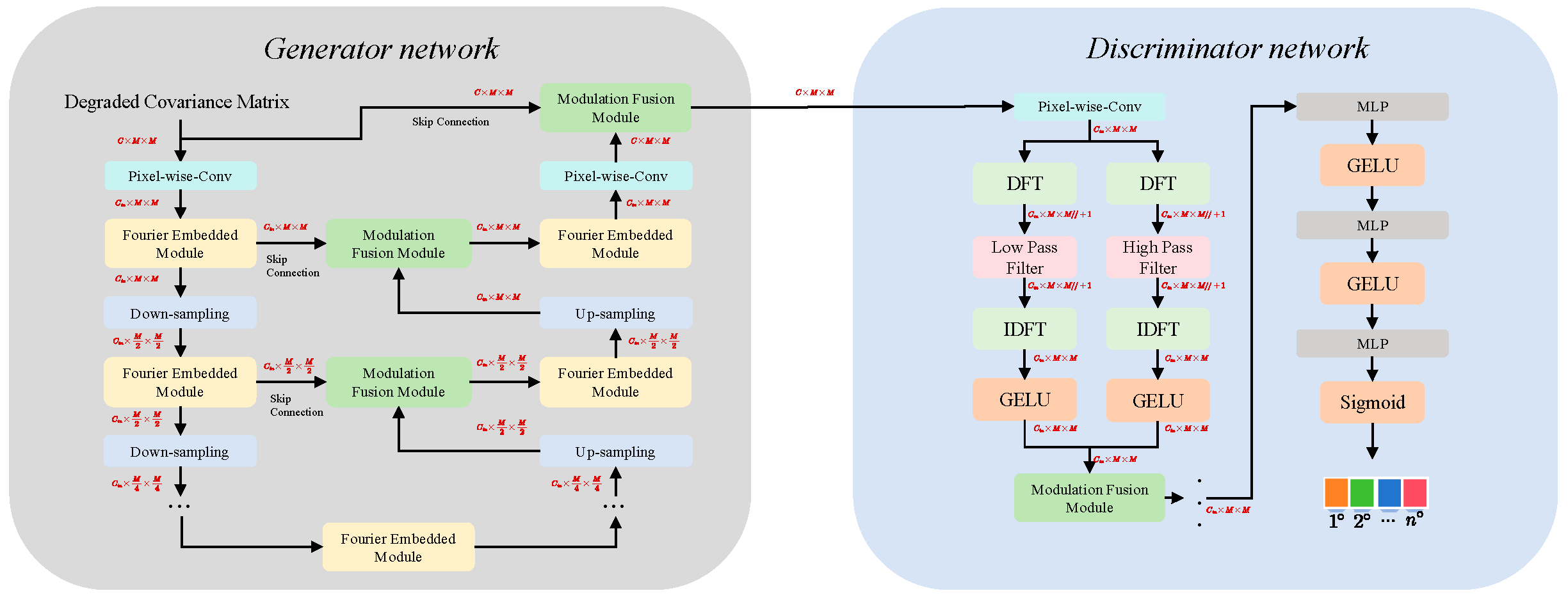
3.2. Neural Network Structure

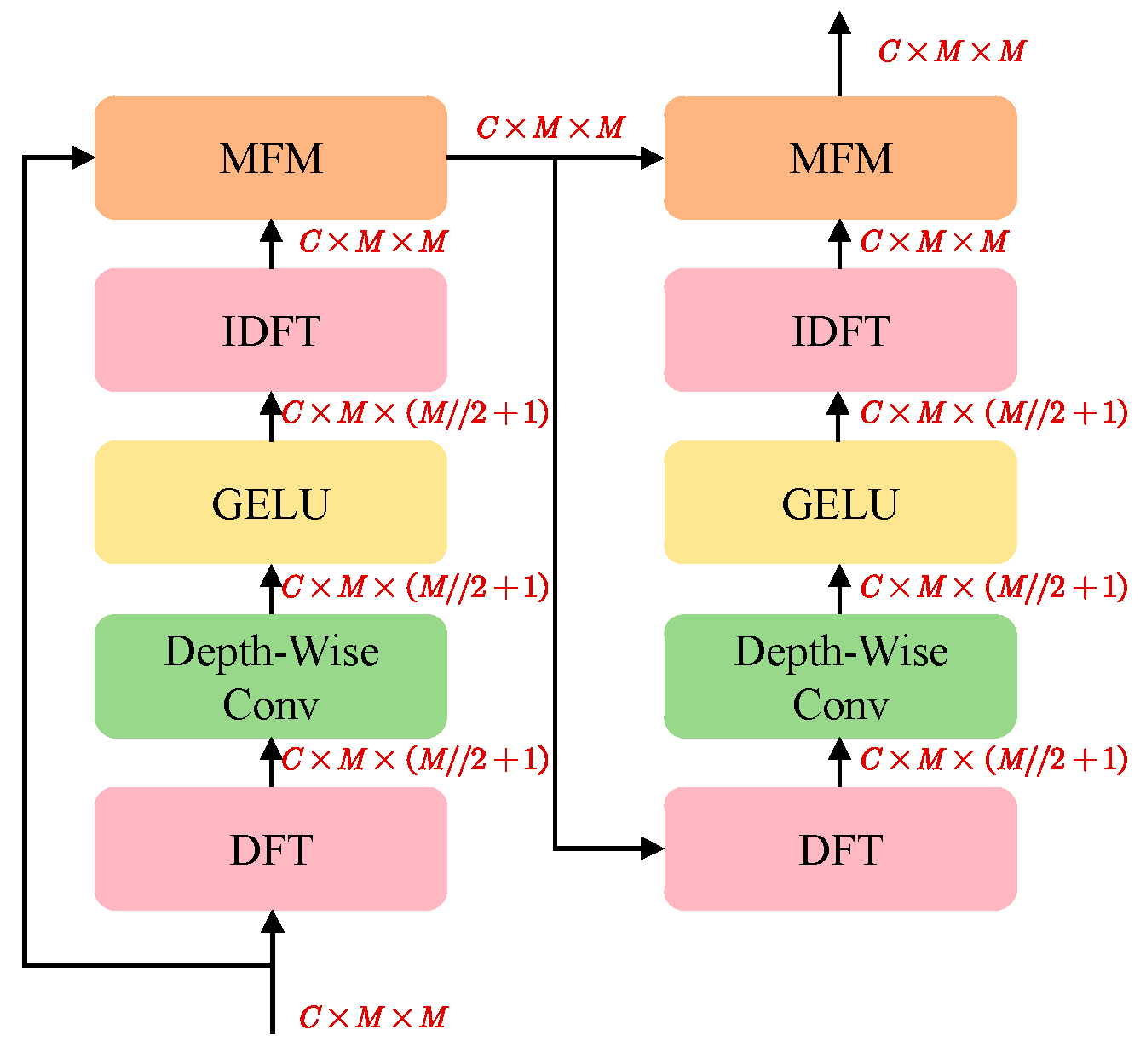
3.2.1. Generator Network Structure

Deep learning is widely used in computer vision engineering practice, aiming to solve classification, regression, and other problems. In order to solve the DOA estimation problem under low SNR, this paper proposes a deep learning algorithm based on DAE with Discrete Fourier Transform and Deep Feature Fusion. DAE [38,39] is a variant of Autoencoder (AE). The difference is that DAE performs feature learning by training the corrupted data after adding noise and uses the input original data and the output denoized data to calculate the loss function and perform error back-propagation. The specific process is illustrated in Figure 2.

The primary objective of the DAE is to restore noise-corrupted covariance matrices, as detailed in Figure 1. Given an input covariance matrix $\mathit{R}\in 2\times M\times M$, the process begins with a pixel-wise convolutional layer to transform the raw data into high-dimensional features ${\mathit{R}}_{conv}\in 128\times M\times M$. We design a U-shaped network architecture with skip connections and a Modulation Fusion Module (MFM) [40], implementation details in Figure 3 to mitigate gradient vanishing and ensure the restored matrix retains richer original information. The network comprises N = 4 encoder stages, each containing a Fourier Embedded Module (FEM) [41], implementation details in Figure 4, and a 3 × 3 convolutional down-sampling layer with stride 2. Symmetrically, the decoder employs stacked FEM and a 3 × 3 Transposed Convolution Layer with stride 2, padding 1 up-sampling layers for feature reconstruction. Finally, a pixel-wise convolutional layer generates a residual matrix ${\mathit{R}}_{res}\in 2\times M\times M$, which is added to the degraded matrix to produce the final restored result.

Compared to direct residual connections, which simply add input and output features, the MFM module enhances feature refinement by generating channel-spatial attention weights through Global Average Pooling (GAP), Multi-layer Perceptron (MLP), and Softmax. These weights dynamically adjust the contributions of different frequency components, effectively suppressing noise while amplifying discriminative features. Furthermore, within encoder–decoder architectures, the MFM enables adaptive fusion of low-frequency information from deep encoder layers with high-frequency details from shallow decoder layers. This mechanism not only improves model performance but also accelerates network convergence by optimizing gradient propagation across hierarchical features.

By applying the DFT, input features $R\in {\mathbb{R}}^{C\times M\times M}$ of FEM are decomposed into real $R_{\mathcal{I}}$ and imaginary $R_{\mathcal{R}}$ components, which undergo spatial interaction modeling through Depth-Wise Convolutions (DWConv) [42,43] with the kernel size of 3 × 3, stride 1, padding 1, and Gaussian Error Linear Unit (GELU) activation. The corresponding Fourier transform is expressed as

$$R_{\mathcal{I}}^{\left(b\right)},R_{\mathcal{R}}^{\left(b\right)}=DFT\left(R^{\left(b\right)}\right)=\sum _{k=0}^{M-1}\sum _{l=0}^{M-1}{R}^{\left(b\right)}\left[k,l\right]\cdot {\mathrm{e}}^{-\mathrm{j}2\mathsf{\pi }\left({\displaystyle \frac{pk}{M}}+{\displaystyle \frac{ql}{M}}\right)}$$

(8)

where batch size $b=1,2,...,B$, $R_{\mathcal{I}}^{\left(b\right)} \mathrm{a}\mathrm{n}\mathrm{d} R_{\mathcal{R}}^{\left(b\right)}$ indicate the real and imaginary, respectively.

The filtered frequency-domain features are then restored to the spatial domain via inverse DFT (IDFT) and concatenated with spatial features processed by half-instance normalization, generating the final output. Leveraging the global frequency representation of Fourier transforms, this method explicitly suppresses high-frequency noise while enhancing low-frequency structures in the frequency domain, complemented by spatial detail refinement for cross-domain synergy. Compared to conventional residual connections, through dynamic frequency-aware weighting and cross-level feature fusion, while maintaining computational efficiency comparable to spatial convolutions.

3.2.2. Discriminator Network Structure

For a multi-label classification model based on DOA estimation, in order to enhance the network’s classification performance, we employ a series of DFT modules to extract high-frequency and low-frequency features from the covariance matrix. These features are then adaptively fused through a MFM with learned weights, and the integrated representation is ultimately fed into a sequence of MLP to generate the classification results.

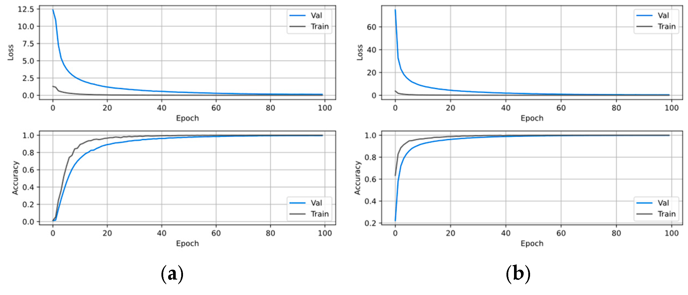
3.3. Network Training

We divide the training process into two steps. In the first step, we conduct unsupervised training on the DAE to enhance the network’s ability to suppress noise of varying intensities. In the second step, we freeze the batch normalization layers in the DAE and perform supervised training on the discriminator network to find the optimal weights for DOA estimation.

We considered two scenarios: (i) setting ${\phi }_{\mathrm{m}\mathrm{a}\mathrm{x}}=60°$ which defines the wide grid set $\Omega =\left\{-60,-59,\dots ,59,60\right\}$ for number of source K =1 or 2, and (ii) setting ${\phi }_{\mathrm{m}\mathrm{a}\mathrm{x}}=30°$, which defines the narrow band $\Omega =\left\{-30,-29,\dots ,29,30\right\}$ for source K = 3. This configuration does not affect the network architecture of the DAE, but the output dimension of the last MLP in the discriminator network needs to be adjusted accordingly. Specifically, the output dimension for the wide-band scenario is set to 121, while that for the narrowband scenario is set to 61. The remaining parts of the network remain unchanged.

The discriminator network corresponding to these two modes need to be trained separately. At the same time, we trained the discriminator network separately based on the different levels of prior knowledge. Initial investigations address scenarios with a priori known source cardinality, specifically analyzing dual-source interference regimes $K=2$ and triple-source resolution challenges $K=3$. The subsequent analysis proceeds to address realistic operational conditions where source cardinality must be jointly estimated, testing the framework under blind enumeration constraints. In this case, the dataset includes cases where K = 1, 2, and 3, and the network is utilized to simultaneously estimate the number of sources and the DOA.

3.3.1. Generator Network Training

The DAE network was trained using unsupervised DAE training. The array-received signal under the classical array signal model was used as the data set source, and the real and imaginary parts of the covariance matrix of the array-received signal were used as the network input to construct the data set. Below is a brief description of the data set generation process and method.

To improve the network’s generalization performance across different SNRs, we add noise of varying powers to the original data, resulting in $SNR=\left\{-20,-15,-10,-5,0,5,10\right\}\mathrm{dB}$. We train the DAE using a mixed number of sources, with corresponding numbers of samples $C_{121}^1=121$, $C_{121}^2=7260$, and $C_{61}^3=35990$ for K = 1, 2, and 3, respectively. The final dataset size is 216,855. The dataset is split into training, testing, and validation sets in a 7:2:1 ratio.

We employ the Adam optimizer to update the network parameters, with a learning rate of 0.001, and train for 100 epochs. We adopt a cosine annealing strategy to reduce the learning rate during training. The learning rate for each cycle (or wave) can be expressed as

$${\eta }_t={\eta }_{\mathrm{m}\mathrm{i}\mathrm{n}}+{\displaystyle \frac{1}{2}}\left({\eta }_{\mathrm{m}\mathrm{a}\mathrm{x}}-{\eta }_{\mathrm{m}\mathrm{i}\mathrm{n}}\right)\cdot \left(1+\mathrm{c}\mathrm{o}\mathrm{s}\left({\displaystyle \frac{\pi t}{T_{\mathrm{m}\mathrm{a}\mathrm{x}}}}\right)\right)$$

(9)

3.3.2. Discriminator Network Training

The discriminator part is also trained under a SNR ranging from −20 to 0 dB with a step size of 5 dB. When the number of sources is fixed, the dataset sizes are $D=5\times 7260=36,300$ and $D=5\times 35,990=179,950$ for K = 2 and K = 3, respectively. For blind source enumeration scenarios, we set ${\phi }_{\mathrm{m}\mathrm{a}\mathrm{x}}=30°$, which means $\left|\Omega \right|=61°$. The size of the dataset is $D=5\times \left(C_{61}^1+C_{61}^2+C_{61}^3\right)=189,405$. The network’s training parameters are the same as before, except for the batch size, which is reduced to 64. In Figure 5, we have plotted the network training process for a fixed number of sources, where (a) corresponds to two sources and (b) corresponds to three sources.

4. Simulation Results

In this section, we conduct several experiments to evaluate the DOA estimation performance of the proposed DFNeT method under different scenarios. Firstly, we verify the denoising performance of the DAE. Secondly, we examine the performance of the proposed method under the assumption that the number of sources is known, specifically for one, two, and three sources. The network undergoes multi-cardinality training with source count heterogeneity up to $K_{\mathrm{m}\mathrm{a}\mathrm{x}}=3$.

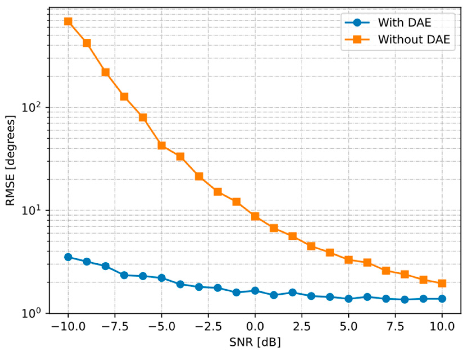
4.1. Performance of DAE

We set the number of array elements to 16 and the spacing between elements at the half-wavelength distance $d=\lambda /2$. The training strategy is as described above in Section 3.3.1. The noise variance is reasonably set to achieve an input data SNR within the range of [−10, 10] dB with step of 1. In Figure 6, we systematically investigated the variations in RMSE between noise-degraded covariance matrices and their original counterparts under different SNR conditions. The study specifically compared the results obtained with and without the application of a DAE. The simulation results in below Figure 6 demonstrate the superior denoising capability of the proposed DAE against additive white Gaussian noise (AWGN), particularly evidenced by significant RMSE reduction in low SNR regimes.

4.2. Comparison to Other Methods

We compare the performance of the proposed method with the following methods:

• MUSIC in [1]
• Root-music in [44,45]
• ESPRIT in [2]
• UnESPRIT in [46]
• CNN in [27]

Methods (a–d) are well-established in the DOA estimation literature and serve as benchmarks to evaluate the effectiveness and advantages of the proposed method. Method e is a deep learning-based DOA estimation method with superior performance. The grid resolution for all methods (MUSIC, CNN in [27], and proposed method) is set to $\rho =1°$. We have also calculated the Cramér-Rao Bound (CRLB) [47] for uncorrelated signals in [48]. By comparing the performance of the proposed method with these classic approaches, we can gain insights into its strengths and potential areas for improvement.

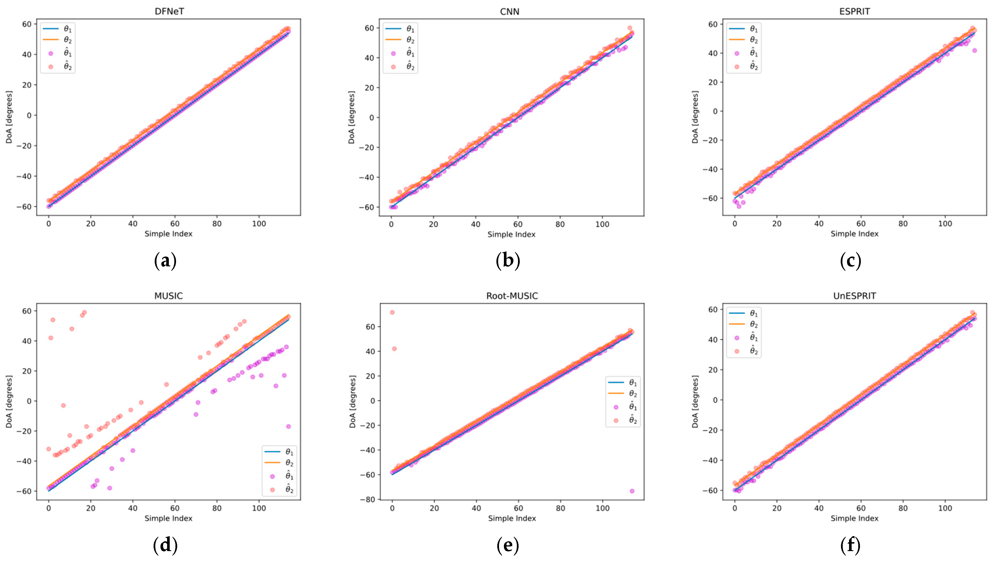
4.3. Operational Performance with Two Simultaneous Emitters

4.3.1. Cross-Method Performance Benchmarking

This section establishes a controlled two-source scenario with a fixed angular separation of $∆\theta =3.4°$. The first target ${\theta }_1$ is located on-grid with a range of $\left[-60°,54°\right]$ degrees with a stepwise progression of $1°$, and the second target is located off-grid with ${\theta }_2={\theta }_1+∆\theta$. The simulations are conducted under the conditions of $SNR=-10 \mathrm{d}\mathrm{B}$ and $T=2000$. Figure 7a presents the estimation results of the proposed method. Figure 7b–f present the MUSIC, Root-MUSIC, ESPRIT, UnESPRIT, and CNN in [27], respectively. Finally, the estimate errors’ absolute error and RMSE of all the above methods are presented in

Table 1. RMSE of all Methods with two fix angles.

Methods	Absolute Error	RMSE	Runtime
MUSIC	71.0	18.156996495542	5.2713 × 104 s
Root-MUSIC	127.33102461862	13.559954773844	4.4995 × 104 s
ESPRIT	12.205500438346	1.3089848606459	1.1502 × 104 s
UnESPRIT	2.6026574864040	0.6014306026930	3.6746 × 104 s
CNN in [27]	4.0	1.1791669867362	2.2422 × 104 s
DFNeT	0.4	0.0304347826086	2.6461 × 104 s

. We have observed that the estimation errors of the proposed method are the smallest, in terms of both the RMSE and the absolute error. The MUSIC method exhibits significant measurement errors at the boundaries, making it almost impossible to accomplish the estimation task. ESPRIT generally exhibits good accuracy, but also suffers from the problem of large errors at the edges. One possible reason is the broadside effect of a ULA, where the rate of change of phase difference accelerates as the direction vector approaches 90 degrees in angle. Meanwhile, the signal energy distribution near the edge angles is weaker, making it more sensitive to noise and interference, which leads to an increase in estimation errors. This issue has been partially addressed in Root-MUSIC and UnESPRIT. Root-MUSIC and UnESPRIT generally have smaller estimation errors, but there is still a certain degree of fluctuation, and their estimation accuracy is inferior to that of the proposed method. Compared with the aforementioned model-based DOA estimation methods, CNN in [27] exhibits a more stable distribution of estimation errors without outliers. However, its measurement accuracy is still not satisfactory.

We have observed that the estimation errors of the proposed method are the smallest, in terms of both the RMSE and the absolute error. The MUSIC method exhibits significant measurement errors at the boundaries, making it almost impossible to accomplish the estimation task. ESPRIT generally exhibits good accuracy, but it also suffers from the problem of large errors at the edges. One possible reason is the broadside effect of a uniform linear array, where the rate of change of phase difference accelerates as the direction vector approaches 90 degrees in angle. Meanwhile, the signal energy distribution near the edge angles is weaker, making it more sensitive to noise and interference, which leads to an increase in estimation errors. This issue has been partially addressed in Root-MUSIC and UnESPRIT. Root-MUSIC and UnESPRIT generally have smaller estimation errors, but there is still a certain degree of fluctuation, and their estimation accuracy is inferior to that of the proposed method. Compared with the aforementioned model-based DOA estimation methods, CNN in [27] exhibits a more stable distribution of estimation errors without outliers. However, its measurement accuracy is still not satisfactory.

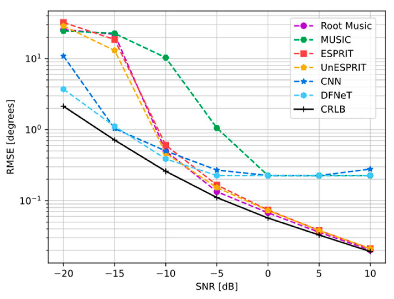
4.3.2. RMSE Under Different SNR with K = 2

In this section, we analyze the estimation accuracy of the proposed method for targets at two fixed directions ${\theta }_1=12.21°,{\theta }_2=14.32°$ under different SNRs $\left[-20,10\right]$ dB with a step of 5 dB. The RMSE for each SNR is calculated with 1000 Monte Carlo trials, where the sample covariance is estimated under T = 1000 snapshots. The results are plotted in Figure 8. At the same time, we also calculated the CRLB for each SNR to evaluate the performance of all the methods. It can be observed that the proposed method exhibits good robustness, with estimation results being minimally affected by noise. In low SNR regions $SNR\in \left[-20,0\right]\mathrm{d}\mathrm{B}$, the overall performance of the proposed method is superior to the deep learning DOA estimation method presented in [27]. Meanwhile, the experimental results indicate that in the high SNR regime, all on-grid methods encounter RMSE floor, while only off-grid methods such as Root-MUSIC, ESPRIT, and UnESPRIT can approach the CRLB. As inherent quantization artifacts plague all grid-based methods, achieving sub-grid accuracy necessitates finer angular meshing—invariably increasing computational complexity.

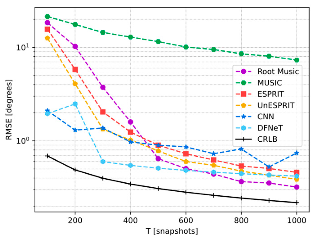
4.3.3. Parametric RMSE Dependence on Snapshot Quantity with K =2

This section quantifies the method’s convergence behavior under finite-snapshot constraints. We fix the $SNR=-10 \mathrm{d}\mathrm{B}$ and set the directions of the two targets as ${\theta }_1=15.18°$ and ${\theta }_2=18.78°$ (off-grid angles). The snapshot count T is systematically varied across the geometric progression $\left\{100,200,\dots ,1000\right\}$ with step size $∆T=100$. Figure 9 depicts experimental results revealing that DL-based estimation methods exhibit stronger adaptability to low snapshot numbers compared to model-driven methods. Meanwhile, except for the case where the number of snapshots $T=200$, where the performance of our proposed method is inferior to that of the method proposed in [27], our method outperforms it in all other scenarios. A critical limitation emerges in snapshot-constrained scenarios: at counts ≤200, noise contamination in covariance matrices significantly impacts estimation accuracy (RMSE of $1.14°$ observed at 200 snapshots in Figure 9). This motivates our ongoing research into snapshot-efficient DOA frameworks.

4.3.4. Dual Stochastic Angular RMSE Performance

In this experiment, we adopt uniformly random angles. Specifically, both ${\theta }_1$ and ${\theta }_2$ follow a uniform distribution form distribution from $p\left(\theta \right)=\mathcal{U}\left(\theta ;-60,50\right)$. For each SNR, there are 1000 random angle samples, with the SNR ranging from −20 dB to 10 dB in intervals of 5 dB. The results are presented in Figure 10. It can be observed that, except for slightly inferior performance in certain SNR regions, such as −20 dB, 0 dB, and 10 dB, compared to other methods, the proposed DFNeT approach has achieved a certain degree of improvement in estimation performance. A plausible explanation is that the DFNeT’s higher architectural complexity relative to CNN necessitates more extensive training data for stable convergence. In the two target scenarios under discussion, insufficient training samples lead to suboptimal convergence behavior in DFNeT, consequently causing fluctuations in estimation accuracy. Refining the SNR sampling interval from 5 dB to 1 dB to expand the training dataset scale will help resolve the aforementioned performance issues.

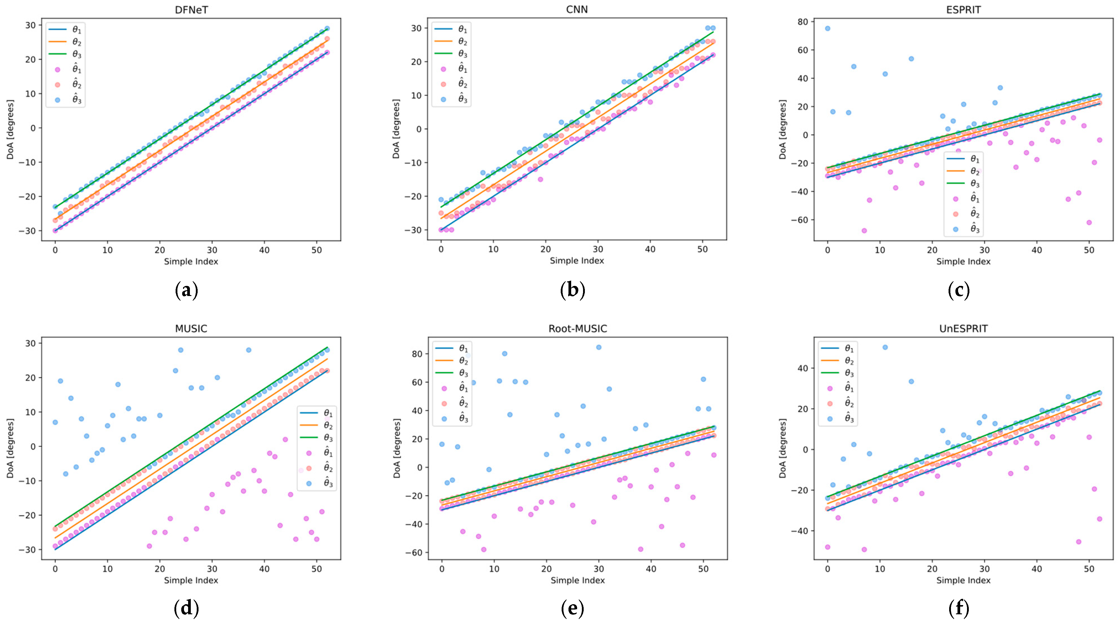
4.4. Results with Three Sources

4.4.1. Comparison of Different Methods

In this section, to further verify the super-resolution performance of the proposed method and its ability to resolve multiple targets, we consider three signals with fixed angular separations with $∆\theta =3.4°$. Meanwhile, in order to reduce the amount of data, we set the angular range to the narrowband range $\Omega \subseteq \left\{-30°,30°\right\}$, as mentioned in Section III-C above. The first target ${\theta }_1$ is located on-grid with a range of $\left[-30°,23°\right]$ degrees with an increasing step $1°$, and the other targets ${\theta }_2,{\theta }_3$ are located off-grid with ${\theta }_2={\theta }_1+∆\theta$, ${\theta }_3={\theta }_1+2\times ∆\theta$, respectively. The other experimental conditions remain the same as those mentioned in Section 4.3.1 above. The simulation results are presented in Figure 11 and

Table 2. RMSE of all methods with three fix angles.

Methods	Absolute Error	RMSE	Runtime
MUSIC	47.0	13.342324012813	5.4774 × 104 s
Root-MUSIC	70.95549396180607	22.791004616156	4.6732 × 104 s
ESPRIT	81.96869387724863	17.588607263825	1.1574 × 104 s
UnESPRIT	63.42179344323082	10.608104099319	1.1451 × 104 s
CNN in [27]	4.0	1.3754358943153	1.1978 × 104 s
DFNeT	2.799999999999997	0.0226415094339	1.2814 × 104 s

.

It can be observed that, except for the deep learning-based estimation method, all the traditional methods such as MUSIC, Root-MUSIC, ESPRIT, and UnESPRIT exhibit significant errors. From the experimental results, it can be seen that although the proposed method’s more sophisticated architecture does not yield significant runtime improvements compared to Root-MUSIC, ESPRIT, and CNN implementations, it achieves superior estimation accuracy. In terms of the absolute error, the proposed method achieves an absolute error of $2.8°$, while the RMSE of CNN in [27] is $3.8°$. The performance of other traditional methods is severely affected:$47.0°$ for MUSIC; $70.9°$ for Root-MUSIC; $81.9°$ for ESPRIT; and $63.4°$ for UnESPRIT. In terms of the RMSE, the proposed method has a minimum RMSE of $0.02°$, whereas MUSIC has a RMSE of $13.3°$; $22.7°$ for Root-MUSIC; $10.6°$ for UnESPRIT. The proposed method exhibits a smaller RMSE and achieves the best performance.

4.4.2. RMSE Under Different SNR with K = 3

In this section, we analyze the estimation accuracy of the proposed method for targets at three fixed directions ${\theta }_1=12.21°$, ${\theta }_2=14.32°$, and ${\theta }_3=16.80°$, under different SNRs at [−20, 10] dB with a step of 5 dB. The simulation results are plotted in Figure 12. In the SNR range of −20 dB to 0 dB, the method proposed in this paper demonstrates significantly superior performance compared to other traditional methods. Additionally, when compared to other deep learning-based methods, the proposed method achieves approximately the same estimation results as the method in [27] in the low SNR region. However, at higher SNRs of 0 dB to 10 dB, the proposed method exhibits improved estimation accuracy compared to [27].

4.4.3. Parametric RMSE Dependence on Snapshot Quantity with K = 3

This experimental investigation quantifies snapshot-dependent performance variations across three distinct target configuration scenarios with ${\theta }_1=11.58°$, ${\theta }_2=15.18°$, and ${\theta }_3=18.78°$. We consider ten cases of snapshot numbers ranging from 100 to 1000 with $∆T=100$, under $SNR=-10 \mathrm{dB}$. Estimation performance is quantified via RMSE, with comparative results detailed in Figure 13. Critical analysis reveals that conventional approaches (MUSIC, ESPRIT, and Root-MUSIC) fail to maintain adequate angular resolution in the specified scenarios where the proposed method achieves sub-degree precision. Additionally, when the number of snapshots is 100, 200, 300, 800, and 1000, the proposed technique achieves lower RMSE than [27].

4.4.4. Triple Stochastic Angular RMSE Performance

In this experiment, we adopt uniformly random angles. Specifically, ${\theta }_1$, ${\theta }_2$, and ${\theta }_3$ follow a uniform distribution form distribution from $p\left(\theta \right)=\mathcal{U}\left(\theta ;-30,30\right)$. For each SNR, there are 1000 random angle samples, with the SNR ranging from −20 dB to 10 dB in intervals of 5 dB. The results are plotted in Figure 14. It can be observed that the proposed DFNeT method has achieved a certain degree of improvement in DOA estimation performance across all SNR regions compared to other deep learning-based methods and model-based methods. Additionally, it is worth noting that, compared to scenarios with two random targets in Section 4.3.4, the proposed method exhibits a smaller RMSE in scenarios with three random targets. In contrast, the estimation performance of other methods declines as the number of sources increases. A plausible explanation for this phenomenon is influenced by the scaling law, which suggests that the amount of training data for scenarios with three targets in the training set is five times that of scenarios with two targets. Consequently, the network demonstrates stronger generalization capabilities for scenarios involving three targets.

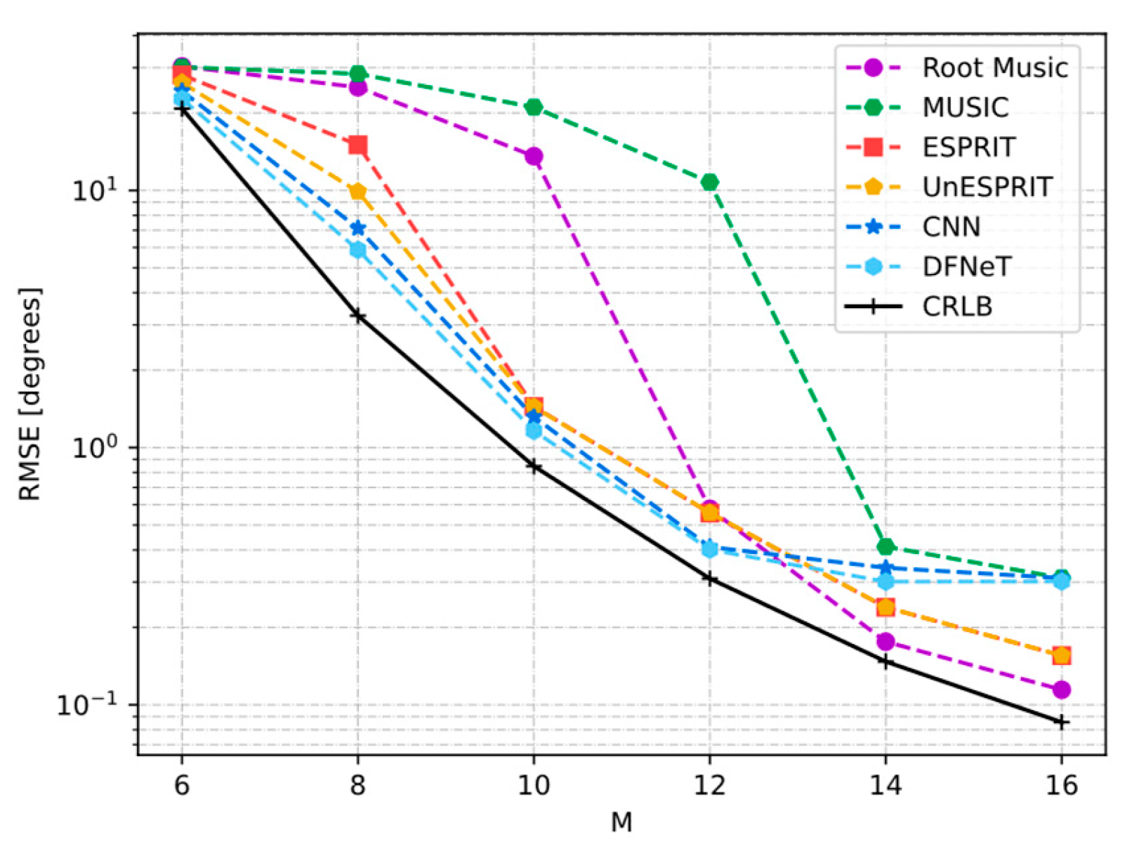
4.4.5. RMSE Under Different Number of Array Elements

This section investigates the impact of varying the number of array elements on model performance. To ensure compatibility with the convolutional and fully connected layers of the neural network, the input covariance matrix is upsampled to dimensions of (16, 16). Simulation conditions are set with a $SNR=0 \mathrm{d}\mathrm{B}$, $T=1000$, and 3 randomly located targets. Six array configurations are tested: 6, 8, 10, 12, 14, and 16 array elements. The CNN model is retrained for each array size scenario, while the proposed DFNeT method retains weights pre-trained exclusively on the 16-element array configuration without retraining. The experimental results are presented in Figure 15. The results indicate that the RMSE of all six methods decreases as the number of array elements increases. Remarkably, the proposed DFNeT method achieves the lowest RMSE across all six scenarios while requiring no retraining.

4.5. Number of Sources Unknown

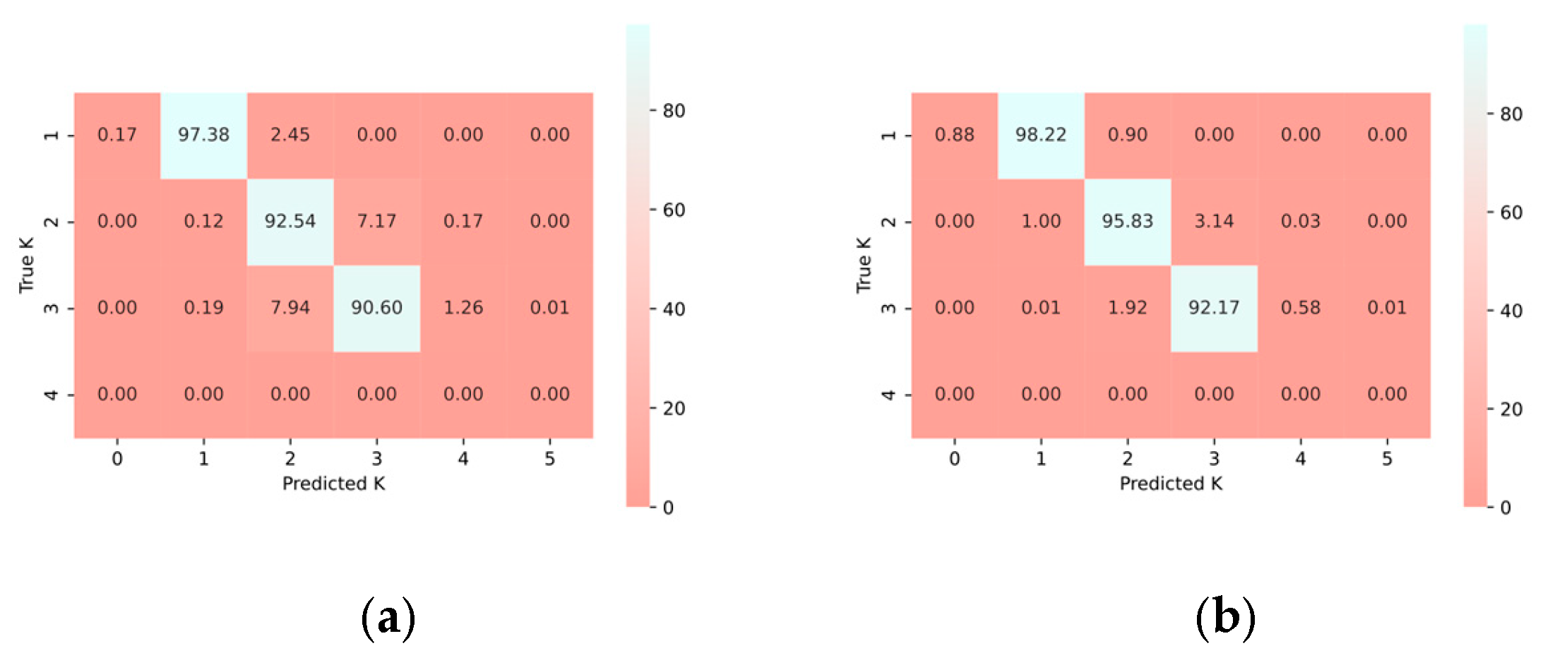
4.5.1. Estimate the Number of Signal Sources

In previous simulations, we typically assumed that the number of signal sources was known, i.e., K = 1, K = 2, or K = 3. Based on this prior information, we selected the maximum K values from the neural network’s output results and used them as the classification results. However, when the number of signal sources is unknown, the above method cannot be implemented. Instead, we adopt the method from [27], which involves setting a confidence level $\overline{p}$ and selecting grid points greater than this threshold as the DOA estimation results. By calculating the average value of the neural network’s output probabilities in a fixed signal source scenario, we set the value of $\overline{p}$ to 0.90. Network classification performance for source enumeration was assessed via confusion matrix analysis under scenarios where the $SNR=-10 \mathrm{dB}$ and $0 \mathrm{dB}$, $T=1000$, and the angles were randomly selected narrowband angles. This evaluation was conducted on 10,000 samples. Figure 16a presents the classification results (probabilities %) at an SNR of −10 dB, while Figure 16b shows the results at an SNR of 0 dB. We observe that, in the majority of cases, the proposed DFNeT exceeds 90% classification accuracy for source cardinalities $K\in \left\{1,2,3\right\}$ under test conditions, as validated by confusion matrix analysis. Furthermore, the proposed method demonstrates superior noise adaptability compared to the approach described in [27].

4.5.2. DOA Estimation with Mix Number of Source

In the final experiment, for the case of $K=1$, we considered validation scenarios comprising angular directions spanning $-29.2°$ to $29.2°$, with an increment step of $1°$. For K = 2, the direction of the first signal ${\theta }_1$ ranged from $-29.2°$ to $27.2°$, and the second signal ${\theta }_2$ was set at an $∆\theta =2.3°$ greater than the first (57 examples), spanning from $-26.9°$ to $29.5°$. For K = 3, the directions of the first two targets ${\theta }_1,{\theta }_2$ remained the same, and the third signal was set at an angle $2.3°$ greater than the second (55 examples), ranging from $-24.6°$ to $29.8°$. The test data were generated at an SNR of −10 dB with a snapshot of T = 1000. Figure 17a–c presents DOA estimation performance under blind source enumeration at $SNR=-10 \mathrm{dB}$. Figure 17a,b demonstrates perfect DOA estimation accuracy (0% false detection rate) for both $K=1$ and $K=2$ sources across all test cases despite the unknown source count at $SNR=-10 \mathrm{dB}$. Figure 17c reveals a single missed detection anomaly in the $K=3$ scenario.

5. Conclusions

This study establishes that while 5G/6G communication systems prioritize spectral efficiency through OFDMA/MIMO techniques at moderate SNRs (0–15 dB), radar systems leverage spread-spectrum processing gain to maintain robust target detection at ultra-low SNRs (≤−15 dB). To bridge this fundamental design dichotomy, we propose DFNeT—a unified deep Fourier transform framework featuring dual innovations: (1) a frequency-domain denoising network that suppresses noise-induced distortions at SNR-critical regimes; and (2) a cross-domain attention module fusing spatial-spectral features for enhanced discrimination. DFNeT achieves breakthrough performance in low SNR positioning for both domains: 63% lower RMSE than CNN at −10 dB, 90% multi-source detection accuracy with 3.4° separation, and 0.03° off-grid consistency under array reconfiguration. The model further demonstrates 94.7% blind source-counting accuracy. By concurrently addressing the SNR adaptability gap and delivering real-time capability, DFNeT enables next-generation positioning for 6G-integrated sensing and radar networks. Future efforts will extend this paradigm to non-uniform arrays and dynamic targets via spatio-temporal-frequency joint optimization.

References

1. Schmidt, R. Multiple emitter location and signal parameter estimation. IEEE Trans. Antennas Propag. 1986, 34, 276–280. [Google Scholar] [CrossRef]
2. Roy, R.; Kailath, T. ESPRIT-estimation of signal parameters via rotational invariance techniques. IEEE Trans. Acoust. Speech Signal Process. 1989, 37, 984–995. [Google Scholar] [CrossRef]
3. Jaffer, A.G. Maximum likelihood direction finding of stochastic sources: A separable solution. In ICASSP-88. International Conference on Acoustics, Speech, and Signal Processing; IEEE Computer Society: New York, NY, USA, 1988; Volume 5, pp. 2893–2896. [Google Scholar]
4. Song, Y.; Zheng, G. Height Measurement for Meter Wave Polarimetric MIMO Radar with Electrically Long Dipole under Complex Terrain. Remote Sens. 2023, 15, 1265. [Google Scholar] [CrossRef]
5. Zheng, G.; Tang, J.; Yang, X. ESPRIT and Unitary ESPRIT Algorithms for Coexistence of Circular and Noncircular Signals in Bistatic MIMO Radar. IEEE Access 2016, 4, 7232–7240. [Google Scholar] [CrossRef]
6. Huang, H.; Yang, J.; Huang, H.; Song, Y.; Gui, G. Deep Learning for Super-Resolution Channel Estimation and DOA Estimation Based Massive MIMO System. IEEE Trans. Veh. Technol. 2018, 67, 8549–8560. [Google Scholar] [CrossRef]
7. Yin, Y.; Wang, Y.; Gong, Y.; Kumar, N.; Wang, L.; Rodrigues, J.J.P.C. Joint multipath channel estimation and array channel inconsistency calibration for massive MIMO systems. IEEE Internet Things J. 2024, 11, 37407–37420. [Google Scholar] [CrossRef]
8. Wang, H.; Xiao, P.; Li, X. Channel Parameter Estimation of mmWave MIMO System in Urban Traffic Scene: A Training Channel based Method. IEEE Transations Intell. Transp. Syst. 2022, 25, 754–762. [Google Scholar] [CrossRef]
9. Zheng, G.; Chen, C.; Song, Y. Height Measurement for Meter Wave MIMO Radar based on Matrix Pencil Under Complex Terrain. IEEE Trans. Veh. Technol. 2023, 72, 11844–11854. [Google Scholar] [CrossRef]
10. Wang, X.; Guo, Y.; Wen, F.; He, J.; Truong, T.-K. EMVS-MIMO Radar With Sparse Rx Geometry: Tensor Modeling and 2-D Direction Finding. IEEE Trans. Aerosp. Electron. Syst. 2023, 59, 8062–8075. [Google Scholar] [CrossRef]
11. Xie, Q.; Wang, Z.; Wen, F.; He, J.; Truong, T.K. Coarray tensor train decomposition for bistatic MIMO radar with uniform planar array. IEEE Trans. Antennas Propag. 2025. [Google Scholar] [CrossRef]
12. Kuang, M.; Wang, Y.; Wang, L.; Xie, J.; Han, C. Localisation and classification of mixed far-field and near-field sources with sparse reconstruction. IET Signal Process. 2022, 16, 426–437. [Google Scholar] [CrossRef]
13. Yin, Y.; Wang, Y.; Dai, T.; Wang, L. DOA estimation based on smoothed sparse reconstruction with time-modulated linear arrays. Signal Process. 2024, 214, 109229. [Google Scholar] [CrossRef]
14. Wang, H.; Xu, L.; Yan, Z.; Gulliver, T.A. Low Complexity MIMO-FBMC Sparse Channel Parameter Estimation for Industrial Big Data Communications. IEEE Trans. Ind. Inform. 2021, 17, 3422–3430. [Google Scholar] [CrossRef]
15. Krizhevsky, A.; Sutskever, I.; Hinton, G.E. Imagenet classification with deep convolutional neural networks. Commun. ACM 2017, 60, 84–90. [Google Scholar] [CrossRef]
16. Simonyan, K.; Andrew, Z. Very deep convolutional networks for large-scale image recognition. arXiv 2014, arXiv:1409.1556. [Google Scholar]
17. He, K.; Zhang, X.; Ren, S.; Sun, J. Deep residual learning for image recognition. In Proceedings of the IEEE Conference on Computer Vision and Pattern Recognition, Las Vegas, NV, USA, 27–30 June 2016. [Google Scholar]
18. Cao, W.; Ren, W.; Zhang, Z.; Huang, W.; Zou, J.; Liu, G. Direction of Arrival Estimation Based on DNN and CNN. Electronics 2024, 13, 3866. [Google Scholar] [CrossRef]
19. Li, N.; Zhang, X.; Lv, F.; Zong, B.; Feng, W. A Bayesian Deep Unfolded Network for the Off-Grid Direction-of-Arrival Estimation via a Minimum Hole Array. Electronics 2024, 13, 2139. [Google Scholar] [CrossRef]
20. Dong, H.; Suo, J.; Zhu, Z.; Li, S. Improved Underwater Single-Vector Acoustic DOA Estimation via Vector Convolution Preprocessing. Electronics 2024, 13, 1796. [Google Scholar] [CrossRef]
21. Xu, X.; Huang, Q. MD-DOA: A Model-Based Deep Learning DOA Estimation Architecture. IEEE Sens. J. 2024, 24, 20240–20253. [Google Scholar] [CrossRef]
22. Hinton, G.E. Reducing the Dimensionality of Data with Neural Networks. Science 2006, 313, 504–507. [Google Scholar] [CrossRef]
23. Burger, H.C.; Schuler, C.J.; Harmeling, S. Image denoising: Can plain neural networks compete with BM3D? In Proceedings of the 2012 IEEE Conference on Computer Vision and Pattern Recognition, Providence, RI, USA, 16–21 June 2012; pp. 2392–2399. [Google Scholar]
24. Papageorgiou, G.K.; Sellathurai, M. Direction-of-Arrival Estimation in the Low-SNR Regime via a Denoising Autoencoder. In Proceedings of the 2020 IEEE 21st International Workshop on Signal Processing Advances in Wireless Communications (SPAWC), Atlanta, GA, USA, 26–29 May 2020; pp. 1–5. [Google Scholar] [CrossRef]
25. Wu, Z.; Wang, J.; Zhou, Z. Two-Dimensional Coherent Polarization–Direction-of-Arrival Estimation Based on Sequence-Embedding Fusion Transformer. Remote Sens. 2024, 16, 21. [Google Scholar] [CrossRef]
26. Cao, Y.; Zhou, T.; Zhang, Q. Gridless DOA Estimation Method for Arbitrary Array Geometries Based on Complex-Valued Deep Neural Networks. Remote Sens. 2024, 16, 3752. [Google Scholar] [CrossRef]
27. Papageorgiou, G.K.; Sellathurai, M.; Eldar, Y.C. Deep Networks for Direction-of-Arrival Estimation in Low SNR. IEEE Trans. Signal Process. 2021, 69, 3714–3729. [Google Scholar] [CrossRef]
28. Shmuel, D.H.; Merkofer, J.P.; Revach, G.; Sloun, R.J.G.V.; Shlezinger, N. SubspaceNet: Deep Learning-Aided Subspace Methods for DoA Estimation. IEEE Trans. Veh. Technol. 2024, 74, 4962–4976. [Google Scholar] [CrossRef]
29. Adavanne, S.; Politis, A.; Virtanen, T. Direction of Arrival Estimation for Multiple Sound Sources Using Convolutional Recurrent Neural Network. In Proceedings of the 2018 26th European Signal Processing Conference (EUSIPCO), Rome, Italy, 3–7 September 2018; pp. 1462–1466. [Google Scholar]
30. Wen, F.; Shi, J.; Gui, G.; Yuen, C.; Sari, H.; Adachi, F. Joint DOD and DOA Estimation for NLOS Target using IRS-aided Bistatic MIMO Radar. IEEE Trans. Veh. Technol. 2024, 73, 15798–15802. [Google Scholar] [CrossRef]
31. Wu, L.-L.; Huang, Z.-T. Coherent SVR Learning for Wideband Direction-of-Arrival Estimation. IEEE Signal Process. Lett. 2019, 26, 642–646. [Google Scholar] [CrossRef]
32. Zheng, R.; Sun, S.; Liu, H.; Chen, H.; Li, J. Interpretable and Efficient Beamforming-Based Deep Learning for Single-Snapshot DOA Estimation. IEEE Sens. J. 2024, 24, 22096–22105. [Google Scholar] [CrossRef]
33. Nie, W.; Zhang, X.; Xu, J.; Guo, L.; Yan, Y. Adaptive Direction-of-Arrival Estimation Using Deep Neural Network in Marine Acoustic Environment. IEEE Sens. J. 2023, 23, 15093–15105. [Google Scholar] [CrossRef]
34. Cho, S.; Jeong, T.; Kwak, S.; Lee, S. Complex-Valued Neural Network for Estimating the Number of Sources in Radar Systems. IEEE Sens. J. 2025, 25, 1746–1755. [Google Scholar] [CrossRef]
35. Xu, S.; Wang, Z.; Zhang, W.; He, Z. End-to-End Regression Neural Network for Coherent DOA Estimation with Dual-Branch Outputs. IEEE Sens. J. 2024, 24, 4047–4056. [Google Scholar] [CrossRef]
36. Gao, N.; Jiang, X.; Zhang, X.; Deng, Y. Efficient Frequency-Domain Image Deraining with Contrastive Regularization. In European Conference on Computer Vision; Springer Nature: Cham, Switzerland, 2024. [Google Scholar]
37. Frigo, M.; Johnson, S.G. FFTW: An adaptive software architecture for the FFT. In Proceedings of the 1998 IEEE International Conference on Acoustics, Speech and Signal Processing, ICASSP’98 (Cat. No. 98CH36181), Seattle, WA, USA, 15 May 1998; Volume 3. [Google Scholar]
38. Gondara, L. Medical Image Denoising Using Convolutional Denoising Autoencoders. In Proceedings of the 2016 IEEE 16th International Conference on Data Mining Workshops (ICDMW), Barcelona, Spain, 12–15 December 2016; pp. 241–246. [Google Scholar]
39. Bengio, Y.; Courville, A.; Vincent, P. Representation Learning: A Review and New Perspectives. IEEE Trans. Pattern Anal. Mach. Intell. 2013, 35, 1798–1828. [Google Scholar] [CrossRef] [PubMed]
40. Zhang, Y.; Zhou, S.; Li, H. Depth information assisted collaborative mutual promotion network for single image dehazing. In Proceedings of the IEEE/CVF Conference on Computer Vision and Pattern Recognition, Seattle, WA, USA, 16–22 June 2024. [Google Scholar]
41. Zhou, M.; Huang, J.; Guo, C.L.; Li, C. An efficient global modeling paradigm for image restoration. In Proceedings of the International Conference on Machine Learning, Honolulu, HI, USA, 23–29 July 2023. [Google Scholar]
42. Howard, A.G.; Zhu, M.; Chen, B.; Kalenichenko, D.; Wang, W.; Weyand, T.; Andreetto, M.; Adam, H. Mobilenets: Efficient convolutional neural networks for mobile vision applications. arXiv 2017, arXiv:1704.04861. [Google Scholar]
43. Chollet, F. Xception: Deep learning with depthwise separable convolutions. In Proceedings of the IEEE Conference on Computer Vision and Pattern Recognition, Honolulu, HI, USA, 21–26 July 2017. [Google Scholar]
44. Rao, B.D.; Hari, K.V.S. Performance analysis of Root-Music. IEEE Trans. Acoust. Speech Signal Process. 1989, 37, 1939–1949. [Google Scholar] [CrossRef]
45. Li, L. Root-MUSIC-based direction-finding and polarization estimation using diversely polarized possibly collocated antennas. IEEE Antennas Wirel. Propag. Lett. 2004, 3, 129–132. [Google Scholar]
46. Haardt, M.; Nossek, J.A. Unitary ESPRIT: How to obtain increased estimation accuracy with a reduced computational burden. IEEE Trans. Signal Process. 2002, 43, 1232–1242. [Google Scholar] [CrossRef]
47. Stoica, P.; Nehorai, A. MUSIC, maximum likelihood, and Cramer-Rao bound. IEEE Trans. Acoust. Speech Signal Process. 1989, 37, 720–741. [Google Scholar] [CrossRef]
48. Jansson, M.; Goransson, B.; Ottersten, B. A subspace method for direction of arrival estimation of uncorrelated emitter signals. IEEE Trans. Signal Process. 1999, 47, 945–956. [Google Scholar] [CrossRef]
Figure 1. General architecture of DFNeT.
Electronics 14 02449 g001
Figure 2. DAE process structure.
Electronics 14 02449 g002
Figure 3. The structure of the MFM.
Electronics 14 02449 g003
Figure 4. The structure of the FEM.
Electronics 14 02449 g004
Figure 5. Training Process: (a) two fix sources, (b) three fix sources.
Electronics 14 02449 g005
Figure 6. Noise reduction effect under different SNRs.
Electronics 14 02449 g006
Figure 7. Off-grid DOA estimation accuracy evaluation at S N R = 10   d B with T = 2000 . Methods of (a) DFNeT, (b) CNN, (c) ESPRIT, (d) MUSIC, (e) Root-MUSIC, (f) UnESPRIT.
Electronics 14 02449 g007
Figure 8. Dual-Source Angular Resolution Characteristics Across SNR Gradients.
Electronics 14 02449 g008
Figure 9. Snapshot-limited Angular Resolution for Dual Sources.
Electronics 14 02449 g009
Figure 10. Dual-Source Error Distribution vs. SNR.
Electronics 14 02449 g010
Figure 11. Off-grid DOA estimation accuracy evaluation at S N R = 10   dB and T = 2000 . Methods of (a) DFNeT, (b) CNN, (c) ESPRIT, (d) MUSIC, (e) Root-MUSIC, (f) UnESPRIT.
Electronics 14 02449 g011
Figure 12. Triple-Source Angular Resolution Characteristics Across SNR Gradients.
Electronics 14 02449 g012
Figure 13. Snapshot-limited Angular Resolution for Triple Sources.
Electronics 14 02449 g013
Figure 14. Triple-Source Error Distribution vs. SNR.
Electronics 14 02449 g014
Figure 15. Performance of DOA estimation of three random sources under different number of array elements.
Electronics 14 02449 g015
Figure 16. Confusion matrix results: (a) SNR = −10 dB; (b) SNR = 0 dB.
Electronics 14 02449 g016
Figure 17. DOA prediction by the DFNeT under number of sources unknown: (a) one fix source; (b) two fix sources; (c) three fix sources.
Electronics 14 02449 g017