Abstract
With the rapid growth of populations worldwide, the need for intelligent crowd management solutions has become increasingly critical. One of the key challenges in this field is accurately assessing and managing pedestrian movement. Traditional crowd management systems rely on localization maps, while topology maps provide an alternative approach to analyzing pedestrian dynamics. In this paper, we explore the integration of virtual coordinate systems (VCSs) with topology maps for enhanced crowd management. We propose a novel mobility model based on the Reference Point Mobility model to simulate pedestrian movement and generate datasets for experimental evaluation. Additionally, we assess the reliability of the VCS in detecting congestion by introducing a method that quantifies node density in a given area. This method estimates a node’s potential location based on the average number of hops between the node and anchor points. Our approach demonstrates promising results, achieving a maximum error rate of 12%.
1. Introduction
The rapid growth of global populations, the increasing frequency of large gatherings due to economic and social factors, and unexpected crises such as pandemics have amplified the need for effective crowd tracking and mobility recognition. Ensuring crowd safety in unpredictable situations is a critical challenge, as human behavior can be highly variable in response to sudden events. This has led to increased interest in studying crowd movement and developing mobility mechanisms to manage large-scale pedestrian flows efficiently. Numerous studies have attempted to address this issue by proposing various solutions for optimizing crowd mobility and safety.
In this paper, we introduce a novel approach to crowd management by integrating Virtual Coordinates (VCs) into mobility models. While Global Positioning Systems (GPSs) are commonly used for tracking movement, they have several limitations in outdoor environments, including data quality issues, signal disturbances, and loss of accuracy. In contrast, VC-based systems offer a more reliable alternative for modeling and managing pedestrian flow in dense environments [1,2,3,4].
VCs are utilized to represent node positions based on hop distances to a set of anchor nodes, offering a scalable and efficient alternative to GPS-based localization [4]. In different applications and scenarios, this characteristic is important due to connection limitation, interference, and/or restriction. In crowd management, pedestrians can experience similar limitations using GPS technology, which necessitate having an alternative VC-based solution.
Our approach aims to take advantage of the VC to be embedded in the models that control mobility behavior and use it in managing crowds and pedestrian flows. The primary contributions of this paper are summarized as follows: (1) integrating Virtual Coordinates (VCs) with mobility models to enhance crowd management, (2) proposing a hybrid mobility model designed to simulate real-world pedestrian movement in crowded environments, and (3) incorporating a novel leader–follower framework, where a leading entity is followed by a group of individuals (nodes/pedestrians), mimicking natural pedestrian behavior in congested areas.
The rest of this paper is organized as follows. Section 2 provides background information and explains many of the terms used in the paper. Section 3 presents a review of the related literature and existing approaches. Section 4 introduces the proposed approach to crowd management. Section 5 provides the experimental design of the proposed approach. Section 6 discusses the performance of the proposed approach. Finally, Section 7 concludes the paper.
2. Background
This section describes several terminologies that are frequently used in different sections of this paper.
2.1. Crowd Management
A crowd can be explained to be a large gathering of people at a specific place while presenting different types of attitudes and behaviors. Managing and tracking this wide range of people in a real environment is more likely to be challenging. This is because of the unpredictable behaviors of people having a chance to change scenarios into an abnormal condition due to any unexpected external incidents that might happen, such as gunfire, fires, or other emergencies, as well as internal ones like overcrowding, where it usually happens to be uncontrollable and has a high chance for a catastrophe consequence [2].
The challenge with managing overcrowded areas is how to safely direct a significant number of pedestrians to avoid bottlenecks at congestion points [3]. Large mass gatherings that congregate in a particular area can sometimes lead to panic and make people’s behaviors more prone to hazards, catastrophes, and even the possibility of death; that is why such situations always require very careful management, since this congestion incurs a lot of physical and digital resources and necessitates the need to ensure public safety and security.
2.2. Virtual Coordinates
Virtual Coordinates (VCs) characterize each node in the network based on its own hop distance to a group of nodes that are called anchors. The performance of a VC system is sensitive to both the number of anchors and their locations within the network [4].
2.3. Virtual Mobility (As a Concept)
Virtual mobility (VM) is a relatively new phenomenon. Accordingly, the definition of the virtual mobility concept may vary across different contexts. In our context, VM is characterized as a complement or as an alternative to physical mobility, particularly in areas such as education, digital collaboration, and remote work. For instance, programs like Erasmus and similar initiatives incorporate elements of virtual mobility, allowing individuals to engage in international academic and professional experiences without the need for physical relocation. VM also encompasses independent mobility that leverages online learning platforms and digital communication networks, enabling seamless global connectivity and interaction [5].
2.4. Mobility Models
This section introduces and discusses the common mobility models found in the literature.
2.4.1. Random Mobility Models
There are several models that belong to this type, which are discussed below:
- Random waypoint model
The random waypoint model is a type of random mobility model which has nodes that move independently to a randomly chosen destination with randomized velocity. Due to its simplicity and wide availability, it has become one of the frequently used models in mobility simulations. However, despite its common use, a fundamental understanding of the random waypoint’s theoretical characteristics is still lacking, and researchers are investigating its stochastic properties [6].
- Random directional model
The random directional model overcomes two key limitations of the random waypoint model: non-uniform spatial distribution and density wave issues. Instead of randomly selecting a destination, nodes in this model choose a random direction within the simulation field and continue moving until they reach the boundary of the field and then pauses for a period; after the pause period, the node then chooses another random direction to travel. This results in a uniform distribution of node movement inside the simulation field [6].
- Random walk model
The random walk model simulates unpredictable mobility patterns by directing node movements in a manner that closely resembles Brownian motion. It shares similarities with the random waypoint model due to its strong randomization of the node movement.
However, unlike the random waypoint model, the random walk model does not store past movement data. At each time interval, nodes randomly and uniformly select a new speed and direction, without considering their previous states. This memoryless property gives the model a distinct advantage in simulating unpredictable mobility scenarios [7].
2.4.2. Geographical Restricted Mobility Models
Another limitation of the random waypoint model is having unconstrained movement, which allows nodes to move freely throughout the simulation field. However, in most real-world scenarios, this freedom is not applicable, but they are more likely to be subjected to their simulation environment; for enhancement, another work was proposed to limit this freedom of motion in the random waypoint model by restricting its movement to a geographical area in the simulation field, which means that these mobility nodes are moving in a pseudo-random way but on a specified pathway inside the simulation area. Some studies address the characteristic and integrate structured pathways and obstacles into those mobility simulations. This category of models is referred to as mobility models with geographic restrictions [6]. Two key geographically restricted models are the pathway and obstacle mobility models, which are discussed next.
- Pathway mobility model
The pathway mobility model gives a more realistic representation of movement for mobile nodes, since it strictly constrains their mobility behavior. Mobile nodes in this model are restricted to predefined pathways and must adhere to traffic regulations within the simulation field [7]. This restriction enhances the model’s ability to simulate real-world movement patterns more accurately.
- Obstacle mobility model
Previously, we discussed the pathway mobility model, which imposes geographic constraints on mobility. Another model that plays an important role in mobility modeling by introducing obstacles within the simulation field is the obstacle mobility model. Mobile nodes require changing their pathways dynamically to avoid the obstacles on the field, significantly influencing their movement behavior [6]. This model enhances realism by simulating real-world mobility challenges such as blocked roads, barriers, or restricted zones.
2.4.3. Temporal Dependency Mobility Models
Physical laws of acceleration can apply constraints on the mobile node. Furthermore, the velocity and rate of change of direction are also affected. Temporal dependency mobility models focus on the dependency between the past, current, and future velocities of a node. Thus, a node’s velocity at a given moment is often correlated with its previous velocity, making it possible to predict future movement trends. This characteristic is referred to as the temporal dependency of velocity.
However, the memoryless nature of the random walk model and random waypoint model render them inadequate to capture the behavior of temporal dependency. As a result, various mobility models considering temporal dependency have been developed [6]. These models can be classified into two major types: the Gauss–Markov model and smooth random model.
- Gauss–Markov model
The Gauss–Markov process is a stochastic process widely used in mobility modeling and other social applications. In terms of continuous time, a stationary Gauss–Markov process can be described by the following autocorrelation function (Equation (1)) [8].
where
Rf(t) = the autocorrelation at lag t (how similar the process is to itself t steps later);
t = the time shift (positive or negative integer);
E() = the Expectation operator (statistical average)
f(t) = value of the process at time step t.
= the variance at zero time shift;
determines the degree of memory in the process.
The Gauss–Markov mobility model is designed with adaptation to randomness, with various levels which can be implemented by using a single tuning parameter [7]. Furthermore, the Gauss–Markov mobility model was designed to take advantage of the temporal dependencies while retaining stochastic properties. Moreover, the Gauss–Markov model yields better performance results than other random mobility models [9].
- Smooth random model
The smooth random model considers the temporal dependency of velocity over various time slots. Moreover, it is also found that the memoryless nature of the random waypoint model may result in unrealistic movement behaviors. This model smoothly transitions speed and direction, avoiding sudden acceleration, deceleration, or sharp turns. Instead, speed and direction change incrementally to better reflect natural movement patterns.
In this model, both the speed and direction of nodes are partly influenced by their previous values, ensuring temporal continuity. The degree of temporal dependency is affected by its acceleration speed and the maximum allowed directional change per time slot [6].
2.4.4. Spatial Dependency Mobility Model
In the spatial dependency model, the movement of a node is influenced by adjacent nodes, and the speeds and directions of mobile nodes are associated with each other [9]. However, in the random waypoint model and other random mobility models, a mobile node moves independently of other nodes. The speed, location, and movement direction of each node are not influenced by surrounded nodes.
In contrast, spatial dependency models recognize that the mobility of a node is influenced by neighboring nodes. Since the velocities of different nodes are correlated in space, this characteristic is referred to as the spatial dependency of velocity [6].
2.4.5. Reference Point Group Model
The Reference Point Group Mobility (RPGM) model represents group-based movement, where mobile nodes are organized into groups. Each group has a center, which can be either a logical center or a group leader node [6]. Thus, each group is composed of one leader and multiple members. The movement of the group leader determines the mobility behavior of the entire group, resulting in a strong correlation among group members [10].
As shown in Table 1, each model described has strengths and limitations based on their characteristics and mobility behavior. Our approach aims to mitigate or at least reduce the limitations of the existing models by offering more flexibility and adaptability to fit our specific research needs.

Table 1.
Models’ characteristics comparison.
3. Related Work
In the latest coordinate systems, they are most likely to rely on the geometrical or geographical coordinates. However, researchers have recently been proposing the use of Virtual Coordinates because they depend on the topology of the network as defined by the connectivity of the nodes, without requiring geographical information. Moreover, with the rise of virtual coordinates systems (VCSs), one of the main issues, which is localization in the network, has been resolved. As discussed in [11], topology maps are different from localization maps.
The relative localization schemes expect the relative distances to be accurate, which results in the absolute position of a subset of nodes, making global localization is realizable. In contrast, in topology maps, what is important is the topology preservation, not the physical distances, to reach the physical layout of the sensor network, i.e., between two topological spaces, there must be a continuous inverse function. The nodes in geographical coordinates lack the awareness of their position geographically in the coordinate system. Instead, virtual coordinates represent nodes by anchors, and each node is defined as its hop-by-hop distance to the rest of the nodes in the anchor. One of the famous algorithms is MS-DVCR, which uses virtual coordinates with four sensor nodes at each corner of the area as the anchor points. Moreover, the authors employing the algorithm used the random waypoint model to conserve the energy used in the network [12]. They provide support for data acquisition regarding several phenomena and events related to pollution and traffic. Furthermore, ref. [13] formulated a reaction–diffusion model with Turing instability to model rumor spread and suggest that it is analogously relevant to modeling crowd behavior, especially panic propagation in space. Similarly, ref. [14] developed a spatial diffusion model to analyze rumor propagation dynamics, emphasizing the shortest path of spread and the impact of governmental interventions. Their findings offer valuable insights into controlling information dissemination within complex networks, which is pertinent to managing crowd behavior.
Furthermore, ref. [10] stated that such wireless widespread deployment leads to the appearance of new services, with one of them being roaming. Particularly in densely covered areas, users tend to roam frequently across different hotspots, e.g., areas covered by one or more networks. However, ref. [12] stated that individual mobility modeling attempts to mimic the mobility pattern behavior of a specific node and in order to understand the networking issues of mobility nodes and the corresponding dynamic characteristics in realistic scenarios, and researchers need to build a suitable mobility model for mobility nodes [6].
Mobility as a concept can be represented by multiple models. First, the random walk mobility model, also known as Brownian motion, is one of the oldest models in place. Random walk is based on a random choice of direction and speed. Moreover, in [12], it is explained as one of the most used models in the research and evaluation of performance from an individual perspective; another feature of this model is that it is memoryless: it does not store speed, path, or any other previous information to use future decision.
The other model is probabilistic random walk, which considers a set of probabilities to determine the next position of a node.
For this, the model considers a matrix that keeps the node’s current position (state 0), the node’s previous position (state 1), and the node’s next position (state 2). Although this model offers other ways to define the previous or next movement of a mobile node, it inherits the main features of random walk and hence does not capture the realistic behavior of nodes in mobile wireless networks [6].
4. The Proposed Approach
This section introduces our proposed approach to crowd management in a predefined path, in which the movement of crowds in the path is tracked using the physical coordinate system (PCS), then the virtual coordinate system (VCS) is utilized to determine each node’s location at a specific time, and then the density of nodes for each area is calculated, which assists in determining the crowded area along the path.
We developed three primary models to test our proposed approach: the mobility in PCS model, the virtual coordinates mapping model, and the nodes density evaluation model. The following subsections explain each model in detail.
4.1. Mobility in PCS Model
This model simulates the movement of groups that follow their leaders to move along a predefined path. Our approach is based on the Reference Point Group Mobility model [10], where each group leader acts as a reference point for the group members, making the group members move next to each other within the path.
The leader of each group is deterministically selected at the beginning of the simulation as the node positioned at the front of the group’s initial location. This ensures consistent behavior and repeatability. The leader’s movement is generated using Algorithm 1, which calculates a valid path toward a sequence of target points defined at the corners of the path polygon. Movement is based on iterative steps that maintain direction toward the next target while avoiding movement outside the physical boundaries of the path. If a calculated step falls outside the permitted area, the direction is adjusted using random corrections.
| Algorithm 1. Leader Movements |
| Input: Path:= Physical path coordinates as polygon; Targets:= Points within on path corners; Output: LeaderMovements:= The physical coordinates (x,y) of the following positions of the leader;
|
In the proposed approach, group members update their positions in relation to their leader’s updated position using Equation (2). This equation introduces small random variations (less than 0.9) to each member’s movement to simulate realistic human movement while maintaining overall group cohesion. It ensures that group members stay within the path’s boundaries by maintaining position updates relative to their leader while adding a small random factor to account for minor variations in movement.
In our model, group movements are restricted to the path’s physical boundaries, and we constantly check that each position remains inside the path. Another restriction applies to the chosen direction of leader movements, where the angle must always be directed toward targets along the path. These targets are defined to guide the leader’s movement through the path to the endpoint. These target locations are positioned at the path corners, where the leader must change direction accordingly. Each leader has a unique set of targets selected from collinear points that lie on the same line at the path corner.
Selecting the leader at the front of each group at the start of the simulation ensures consistency and repeatability under identical conditions. This approach also reduces computational overhead, as the leader is fixed and does not change dynamically. It supports group cohesion, as members follow a stable reference point. In addition, since the leader is guided by known target points, the group is more likely to follow the intended path accurately. Overall, this method enables better coordination and more realistic group behavior, which is essential for reliable crowd simulation and density analysis using virtual coordinate systems.
4.2. Virtual Coordinates Mapping Model
This model is responsible for generating the virtual topology map based on PCs data. It identifies the logical location of each node based on the number of hops from the node to each anchor node. The number of hops is determined by calculating the shortest path from each anchor to the node using Dijkstra’s algorithm. Anchors in this model are selected manually, where the communication range between nodes is set to 2.5 units. This range is selected to ensure connectivity and reliability while preserving sufficient resolution for hop-based distance estimation. It helps prevent graph disconnection and maintains spatial accuracy. A proper selection of communication range depends on network dimensions, as well as the number of nodes and their deployment.
4.3. Nodes Density Evaluation Model
The main objective of the proposed approach is to investigate the possibility of defining zones of congestion using the VCS. To achieve this goal, this model computes the error rate of the approach by calculating the density of nodes in the VCS and comparing it with the results obtained in the PCS.
The density of nodes in the PCS is calculated using Algorithm 2. The number of nodes for each zone is determined by examining the coordinates of each node and identifying the zone that includes those coordinates, thereby updating the number of nodes for that zone.
It is often difficult to determine the physical coordinates of the mobile nodes, so a VCS can be used instead, which is based on calculating the number of hops between a node and another node whose physical location is known. Algorithm 3 shows how the VCS is used to calculate the density of nodes in a given zone.
| Algorithm 2. Nodes Density in PCS |
| Input: ZonesNo:= Total number of zones on the path; Zones:= Zone coordinates; PCmetrix:= physical coordinates matrix of nodes; NodesNo:= Total number of nodes on the path; Output: ZonesDensity:= Density of nodes per zone;
|
| Algorithm 3. Nodes Density in VCS |
| Input: ZonesNo:= Total number of zones on the path; Zones:= Anchors that cover each zone; VCmetrix:= Virtual coordinates matrix of nodes; NodesNo:= Total number of nodes on the path; Output: ZonesDensity:= Density of nodes per zone;
|
5. Experimental Design
This section explains the design of the experiment conducted to test the proposed approach. The experiment consists of three main phases as follows:
- Phase 1: This implements the mobility model, which simulates the movement of nodes in PCS and generates a PCS topology map.
- Phase 2: This generates the VCS topology map.
- Phase 3: This computes and compares the node density in the VCS and PCS and then evaluates the results.
Figure 1 shows the overall flow of our experiment, while the following subsections explain each phase in detail.
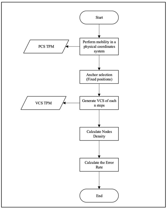
Figure 1.
Flow diagram of experimental design.
5.1. Phase 1
At this phase, the experiment data are collected, which consist of a set of physical coordinates that represent the locations of a group of wireless nodes as they move along a predefined path. Figure 2 shows the motion path for this experiment, which consists of multiple zones. The mobility model was executed multiple times on different numbers of nodes—50, 100, 500, and 1000—to generate the required data samples. For each number of nodes, 9 samples were collected from 9 different zones of the path, with a new sample taken every five steps. To test different network densities and ensure scalability, up to 1000 nodes were simulated. However, this number can be increased depending on the related assumptions on the underlying model.
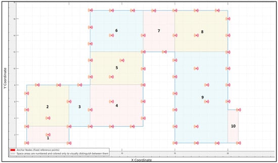
Figure 2.
Movement path, zones, and anchor nodes.
When the mobility model is executed, nodes are deployed at random positions in the first zone of the path. Then, groups are formed by selecting one leader for each member. The closest leader for each member is selected by calculating the Euclidean distance between the member and each leader. In this experiment, leaders represented 4% of the total nodes. This ratio was chosen empirically to ensure manageable group sizes and ability to simulate structured crowd movement.
5.2. Phase 2
This phase processes the data collected in phase 1 to generate the corresponding virtual coordinates. In the experiment, 60 fixed anchor nodes were selected along the path, as shown in Figure 2, most of which were set at the boundaries, while a few were in the middle. The communication range between nodes was set to 2.5. Running this phase resulted in a dataset representing the VCs of the nodes that was then used in phase 3 for analysis.
5.3. Phase 3
In this phase, the density of the nodes in each zone shown in Figure 2 is computed and analyzed. Data collected in phase 1 are used to calculate physical density (PCS-based), while the data collected in phase 2 will be used for calculating the virtual density (VCS-based). Table 2, Table 3, Table 4, and Table 5 show the results of performing this phase on a data sample of sizes 50, 100, 500, and 1000, respectively.
Table 2.
Nodes density results over 9 different time periods (50 nodes).
Table 3.
Nodes density results over 9 different time periods (100 nodes).
Table 4.
Nodes density results over 9 different time periods (500 nodes).
Table 5.
Nodes density results over 9 different time periods (1000 nodes).
6. Key Findings and Performance Discussion
The key findings of the proposed system, presented in comparison with other works, are summarized in Table 6.
Table 6.
Comparison of our proposed approach with existing similar approaches.
The performance of the proposed approach was evaluated using Equation (3) by calculating the average error rate for each zone on the path. It is based on comparing the proportion of nodes in each zone obtained by calculating the density in the PCS with that obtained from the VCS.
where ZD is the zone density, and n is the total number of zones. Figure 3 shows the average error rates for four samples of the dataset.
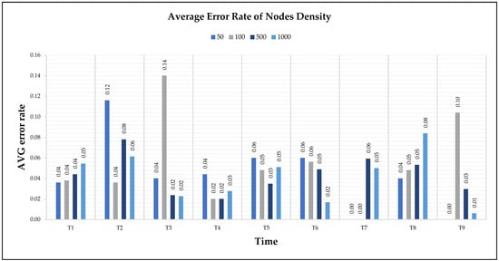
Figure 3.
Average error rate of nodes density.
As shown in Figure 3, the highest error rates obtained by applying the proposed approach were 14% at Time 3 and 10% at Time 9 when performing the experiment on the dataset of 100 nodes, as well as 12% at Time 2 when performing the experiment on the dataset of 50 nodes. The best performance of the proposed approach was when the error rate was 0 at Time 7 and Time 9 when performing the experiment on the dataset of 50 nodes, as well as at Time 7 when performing the experiment on the dataset of 100 nodes.
By comparing these findings with Figure A1, Figure A2, Figure A3 and Figure A4 in the Appendix A, it is clear that the error rate increased when nodes were located on the boundary between two adjacent zones. Resetting the positions of the anchors that defined each zone affected reducing the error rate and calculating the density more accurately.
Figure A1, Figure A2, Figure A3 and Figure A4 in the Appendix A show the locations of the nodes as they moved through the movement path during nine different time periods while running the experiment on datasets of different sizes of 50, 100, 500, and 1000 nodes, respectively. It is noticed by comparing the figures that the movement of the nodes was slower when the path was more crowded. This confirms that higher node densities affect mobility and may cause congestion, which is critical for any crowd management applications.
Table 6 presents a comparative evaluation of the existing research in crowd management, highlighting key aspects such as Virtual Coordinates utilization, mobility modeling, congestion detection, density estimation, and applicability to high-density events like Hajj and Umrah. While prior studies have focused on either density estimation or congestion detection, few have integrated dynamic mobility modeling, and even fewer have incorporated Virtual Coordinates. Notably, our proposed approach outperformed existing methods by integrating all six critical dimensions, offering a comprehensive, scalable, and adaptive solution for real-time crowd monitoring.
By combining Virtual Coordinates with an advanced Reference Point Group Mobility (RPGM) model, our method enhances congestion detection accuracy and ensures efficient pedestrian flow, making it a superior alternative to traditional GPS-based solutions.
7. Conclusions
This paper explores a novel intelligent crowd management approach based on the virtual coordinates system. It increases accuracy and reliability while identifying congestion and tracking mobility. Our approach helps to overcome some of the limitations that traditional systems face, including their reliance on GPS, which has problems with signal interference and inefficient geographic data, by integrating the VCS with the physical coordinates system (PCS) and a Reference Point Group Mobility (RPGM) model; thus, the system offers a more efficient, adaptable, and scalable solution for real-time crowd monitoring.
Experimental results show the effectiveness of VCS-based density estimation, showing that the proposed model can precisely, with low error rates, predict node density along a predefined path. The primary source of minor inaccuracies was the anchor placement, which influenced the density estimation accuracy. Therefore, future improvements can focus on dynamic anchor positioning and extended mobility scenarios to enhance performance in real-world applications.
The main contribution of this work is proposing a novel crowd management approach in scenarios that lack GPS solutions. As urbanization and large-scale public events continue to pose complex crowd control challenges, this VCS-based approach offers a scalable, data-driven solution for ensuring safer and more efficient pedestrian movement in dynamic environments. It provides a structured method for congestion detection and efficient pedestrian flow optimization.
This work is considered valuable for addressing crowd management and modeling movements in VCSs, which can have unlimited applications in communication systems for space, ground, underground, and underwater environments. As a future extension of this work, we suggest dynamic selection and adjustment of the leaders, adaptation to rapid and real-time movements, and improved fault tolerance.
Author Contributions
Conceptualization, N.A.-N. and N.A.; Methodology, N.A.-N., R.K.A. and M.A.; Software, S.J.A. and S.A.; Validation, S.J.A. and M.A.; Formal analysis, S.J.A. and M.A.; Resources, M.A.; Data curation, S.A. and M.A.; Writing—original draft, S.A. and M.A.; Writing—review & editing, N.A.-N., N.A., M.S.I. and A.B.M.A.A.I.; Visualization, S.A.; Supervision, N.A.-N.; Project administration, N.A.-N.; Funding acquisition, N.A.-N. All authors have read and agreed to the published version of the manuscript.
Funding
This work was supported by the Deputyship for Research and Innovation, Ministry of Education, Saudi Arabia, under Project DRI-KSU-762.
Data Availability Statement
The data are contained within the article.
Acknowledgments
The authors extend their appreciation to the Deputyship for Research and Innovation, Ministry of Education, in Saudi Arabia for funding this research work through the project number (DRI-KSU-762).
Conflicts of Interest
The authors declare no conflicts of interest.
Appendix A
This appendix shows the experimental results of running the mobility model on variable size of datasets (nodes), including 50 (Figure A1), 100, 500, and 1000. For each experiment, nine snapshots been taken to represent the location of the mobile nodes during different periods of time (Figure A1, Figure A2, Figure A3 and Figure A4).
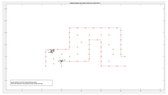
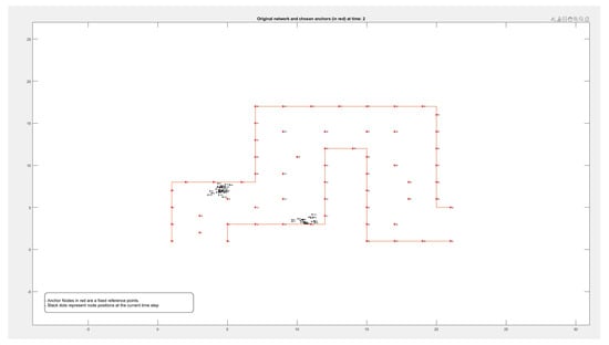
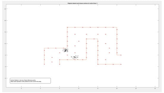
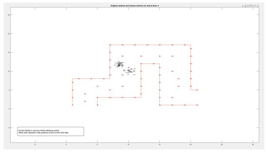
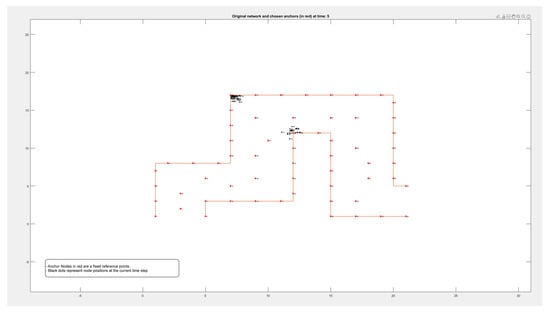
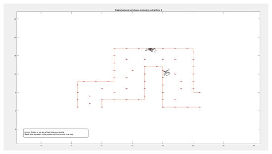
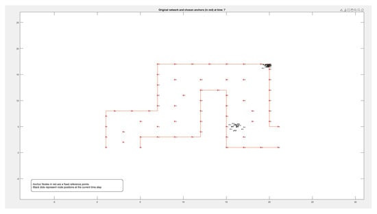
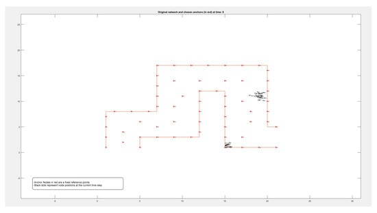
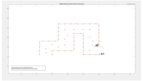
Figure A1.
Locations of 50 nodes moving within a path over 9 different periods of time.
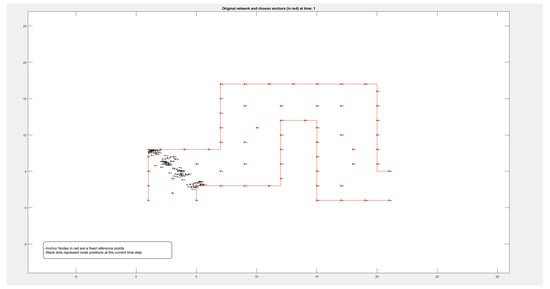
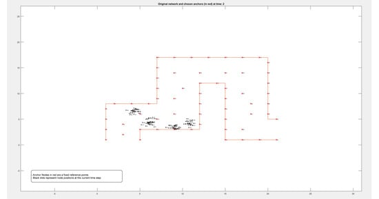
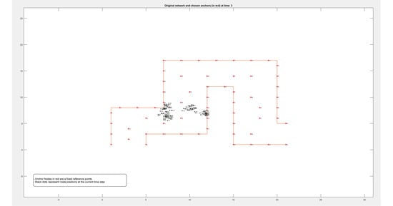
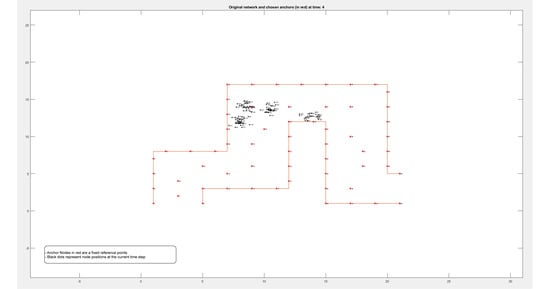
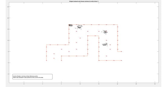
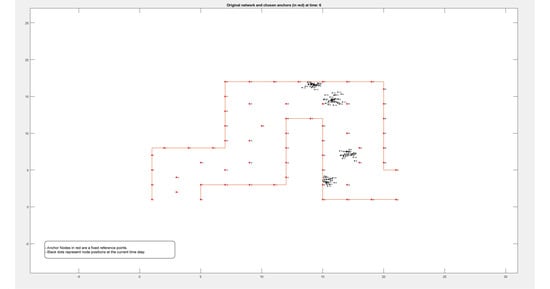
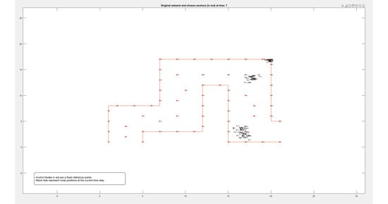
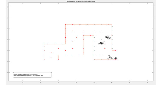
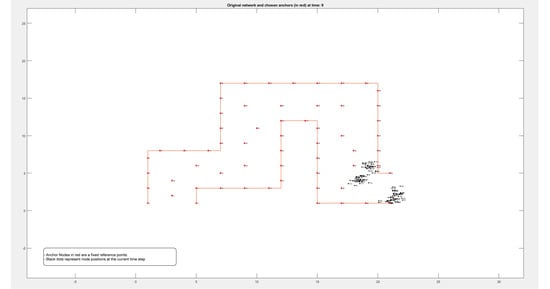
Figure A2.
Locations of 100 nodes moving within a path over 9 different periods of time.
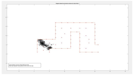
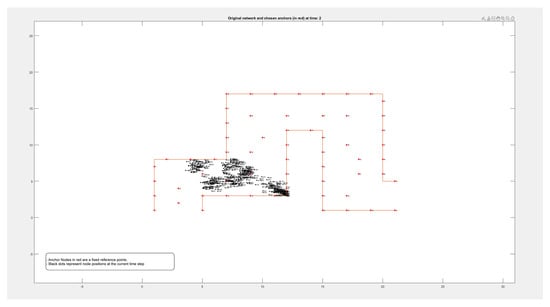
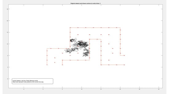
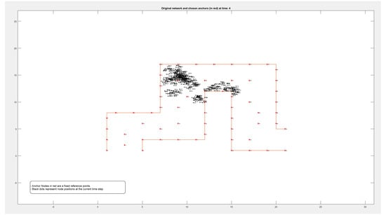
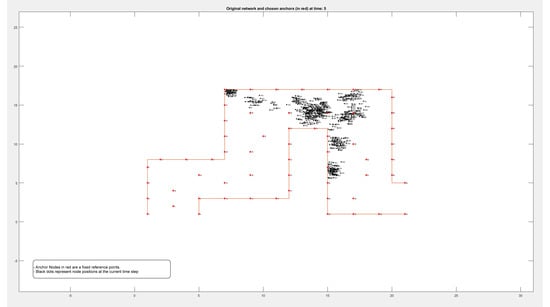
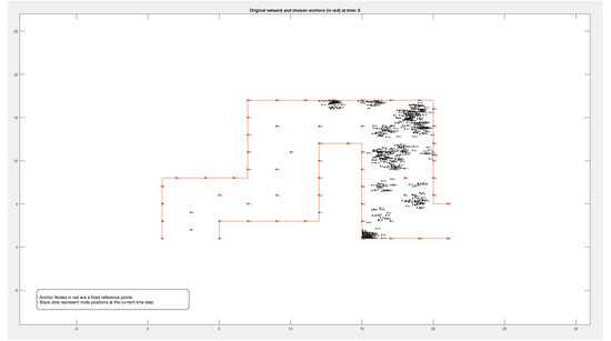
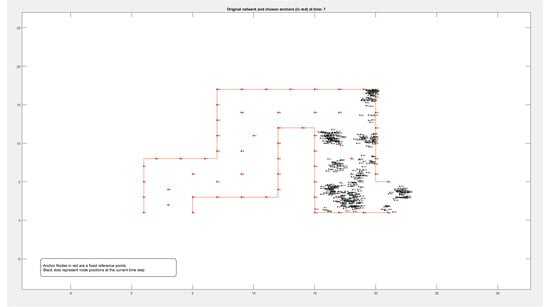
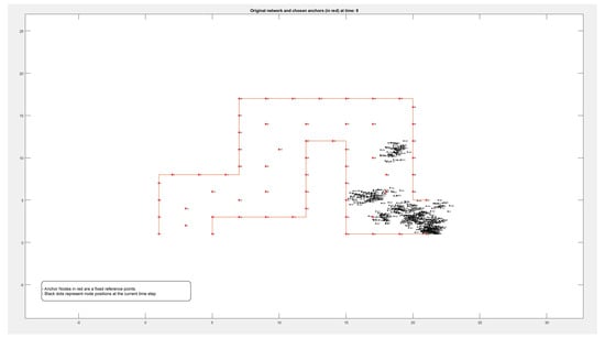
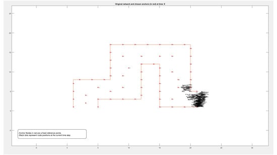
Figure A3.
Locations of 500 nodes moving within a path over 9 different periods of time.
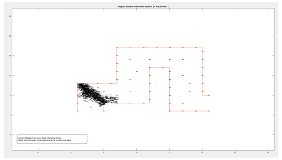
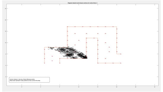
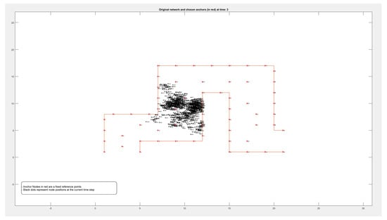
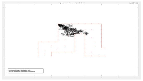

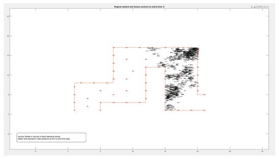
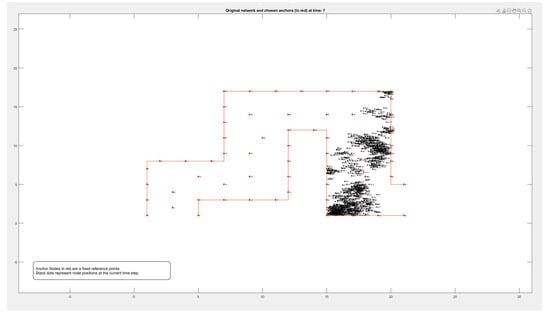
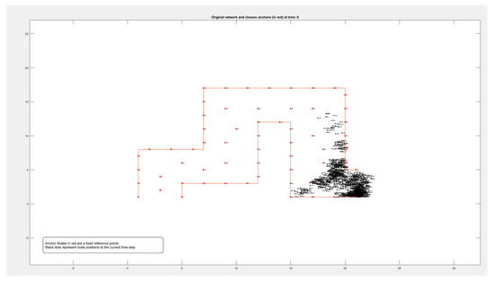
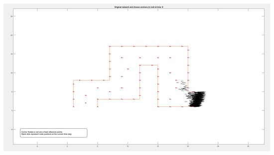
Figure A4.
Locations of 1000 nodes moving within a path over 9 different time periods.
References
- Taczanowska, K.; Muhar, A.; Brandenburg, C. Potential and limitations of GPS tracking for monitoring spatial and temporal aspects of visitor behaviour in recreational areas. In Proceedings of the Fourth International Conference on Monitoring and Management of Visitor Flows in Recreational and Protected Areas, Montecatini Terme, Italy, 14–19 October 2008; Volume 14. No. 19. [Google Scholar]
- Varghese, E.; Thampi, S. Application of Cognitive Computing for Smart Crowd Management. IEEE Access 2020, 8, 43–50. [Google Scholar] [CrossRef]
- Nasser, N.; El Ouadrhiri, A.; El Kamili, M.; Ali, A.; Anan, M. Crowd Management Services in Hajj: A Mean-Field Game Theory Approach. In Proceedings of the IEEE Wireless Communications and Networking Conference (WCNC), Marrakesh, Morocco, 15–18 April 2019. [Google Scholar] [CrossRef]
- Dhanapala, D.C.; Jayasumana, A.P. Anchor Selection and Topology Preserving Maps in WSNs: A Directional Virtual Coordinate-Based Approach. In Proceedings of the 2011 IEEE Local Computer Networks Conference (LCN), Bonn, Germany, 4–7 October 2011; pp. 571–579. [Google Scholar] [CrossRef]
- Daukšienė, E.; Teresevičienė, M.; Volungevičienė, A. Virtual Mobility Creates Opportunities. In Informacinių Technologijų Taikymas Švietimo Sistemoje 2010: E-studijų Patirtis, Aktualijos ir Perspektyvos; Kauno kolegija: Kaunas, Lithuania, 2010; pp. 30–35. [Google Scholar]
- Bai, F.; Helmy, A. A Survey of Mobility Models. In Wireless Ad Hoc and Sensor Networks; Kluwer Academic Publishers: Dordrecht, The Netherlands, 2004; pp. 1–30. Available online: https://www.cise.ufl.edu/~helmy/papers/Survey-Mobility-Chapter-1.pdf (accessed on 6 June 2025).
- Camp, T.; Boleng, J.; Davies, V. A Survey of Mobility Models for Ad Hoc Network Research. Wirel. Commun. Mob. Comput. 2002, 2, 483–502. [Google Scholar] [CrossRef]
- Papoulis, A.; Pillai, S.U. Probability, Random Variables, and Stochastic Processes; McGraw-Hill: Boston, MA, USA, 2002; ISBN 978-0071122566. [Google Scholar]
- Alenazi, M.J.F.; Abbas, S.O.; Almowuena, S.; Alsabaan, M. RSSGM: Recurrent Self-Similar Gauss–Markov Mobility Model. Electronics 2020, 9, 2089. [Google Scholar] [CrossRef]
- Ribeiro, A.; Sofia, R. A Survey on Mobility Models for Wireless Networks. Siti2.Ulusofona.Pt 2011. Available online: https://www.researchgate.net/publication/244478001_A_survey_on_mobility_models_for_wireless_networks (accessed on 10 June 2025).
- Jayasumana, A.P.; Paffenroth, R.; Ramasamy, S. Topology Maps and Distance-Free Localization from Partial Virtual Coordinates for IoT Networks. In Proceedings of the 2016 IEEE International Conference on Communications (ICC), Kuala Lumpur, Malaysia, 22–27 May 2016. [Google Scholar] [CrossRef]
- Rahmatizadeh, R.; Khan, S.A.; Jayasumana, A.P.; Turgut, D.; Bölöni, L. Routing towards a mobile sink using virtual coordinates in a wireless sensor network Science. In Proceedings of the 2014 IEEE International Conference on Communications (ICC), Sydney, NSW, Australia, 10–14 June 2014; pp. 2004–2019. Available online: http://ieeexplore.ieee.org/xpls/abs_all.jsp?arnumber=6883287 (accessed on 3 June 2025).
- Li, B.; Zhu, L. Turing Instability Analysis of a Reaction–Diffusion System for Rumor Propagation in Continuous Space and Complex Networks. Inf. Process. Manag. 2024, 61, 103621. [Google Scholar] [CrossRef]
- Menon, S.; Kumari, S. Impact of Cross-Diffusion and Allee Effect on Modified Leslie–Gower Model. Math. Comput. Simul. 2025, 236, 183–199. [Google Scholar] [CrossRef]
- Kumar, S.; Singhal, A.; Sangal, I.; Bhardwaj, M. Crowd Coordination System. In Proceedings of the 2024 2nd International Conference on Disruptive Technologies (ICDT), Greater Noida, India, 15–16 March 2024; pp. 38–42. [Google Scholar] [CrossRef]
- Halboob, W.; Altaheri, H.; Derhab, A.; Almuhtadi, J. Crowd Management Intelligence Framework: Umrah Use Case. IEEE Access 2024, 12, 6752–6767. [Google Scholar] [CrossRef]
- Macriga, G.A.; Bavyatha, S.; Abhinidhi, S.H.; Jagadeesh, N. Crowd Management Using AI & ML. In Proceedings of the 2024 International Conference on Power, Energy, Control and Transmission Systems (ICPECTS), Chennai, India, 8–9 October 2024; pp. 1–5. [Google Scholar] [CrossRef]
- Villanueva, F.J.; Bolanos, C.; Rubio, A.; Cantarero, R.; Fernandez-Bermejo, J.; Dorado, J. Crowded Event Management in Smart Cities Using a Digital Twin Approach. In Proceedings of the 2022 IEEE International Smart Cities Conference (ISC2), Pafos, Cyprus, 26–29 September 2022; pp. 1–7. [Google Scholar] [CrossRef]
- Shah, A.A. Enhancing Hajj and Umrah Rituals and Crowd Management Through AI Technologies: A Comprehensive Survey of Applications and Future Directions. IEEE Access 2024, 12, 161820–161841. [Google Scholar] [CrossRef]
- Almutairi, M.M.; Apostolopoulou, D.; Stupples, D.; Sen, A.A.A.; Yamin, M.; Halikias, G. Integrative Technologies for Real-Time Crowd Management: A Case Study of the Hajj. In Proceedings of the 2024 11th International Conference on Computing for Sustainable Global Development (INDIACom), New Delhi, India, 28 February–1 March 2024; pp. 203–211. [Google Scholar] [CrossRef]
- He, W.; Pan, G.; Wang, X.; Chen, J.X. Real-Time Crowd Formation Control in Virtual Scenes. Simul. Model. Pract. Theory 2023, 122, 102662. [Google Scholar] [CrossRef]
Disclaimer/Publisher’s Note: The statements, opinions and data contained in all publications are solely those of the individual author(s) and contributor(s) and not of MDPI and/or the editor(s). MDPI and/or the editor(s) disclaim responsibility for any injury to people or property resulting from any ideas, methods, instructions or products referred to in the content. |
© 2025 by the authors. Licensee MDPI, Basel, Switzerland. This article is an open access article distributed under the terms and conditions of the Creative Commons Attribution (CC BY) license (https://creativecommons.org/licenses/by/4.0/).