Powerful Sample Reduction Techniques for Constructing Effective Point Cloud Object Classification Models

Abstract

Due to the large volume of raw data in 3D point clouds, downsampling techniques are crucial for reducing computational load and memory usage to improve the training of 3D point cloud models. This paper plans to conduct research using the ModelNet40 dataset. Our proposed method is based on the PointNext architecture, an improved version of PointNet++ that significantly enhances performance through optimized training strategies and adjusted receptive fields. During the model training process, we employ the farthest point sampling method for downsampling. Specifically, we use an improved attention-based point cloud edge sampling (APES) method for downsampling, where we compute the density of each point and set the size of the neighbor K value to effectively retain feature points during downsampling. Our improved method captures edge points more effectively than the original APES method. By adjusting the architecture, our method, combined with the farthest point sampling method, not only reduced the average training time by nearly 15% compared to PointNext-s, but also improved accuracy from 93.11% to 93.57%.

1. Introduction

The improvement in computational power and the maturity of deep learning technology have gradually shifted the focus of academia and industry from primarily 2D image analysis in the field of computer vision to the study of 3D vision. This shift aims to develop computer vision capabilities in three-dimensional space. In recent years, 3D vision has become a popular research topic, representing the perception and understanding of three-dimensional space. This advancement enables computers and relevant applications to have a more comprehensive understanding of real-world scenes, extending computer vision beyond mere 2D image recognition to include the understanding of object shapes, depths, and spatial positions.

As computer vision and deep learning continue to evolve, 3D point cloud processing has become a hot research topic. The precision of sensors in acquiring point clouds has significantly improved, and the prevalence of 3D scanning devices, such as smartphone 3D applications, stereo cameras, and time-of-flight (ToF) sensors, has increased. This trend has made point cloud acquisition more common in everyday life. Among various applications, 3D point cloud classification and segmentation models play crucial roles in autonomous driving, robotic perception, and virtual reality. However, due to the complexity and diversity of 3D point clouds, existing classification models face several challenges, such as insufficient capture of local details and convergence issues during model training.

The PointNet method [1] was the first to address the disorder problem in point clouds, successfully capturing global feature vectors of the entire point cloud. However, PointNet cannot effectively extract local features. PointNet++ [2], the successor of PointNet, successfully extracts local features. PointMLP [3] follows the design philosophy of PointNet++ but makes the network deeper and simpler. Obtaining finer local features and better learning models remains a hot research direction in recent years. We adopt the PointNext model [4], which optimizes the PointNet++ architecture by improving training optimization strategies and adjusting the receptive field, thereby enhancing its performance and accuracy.

In 3D point clouds, the volume of raw data is enormous, making subsample methods essential during the model training process to reduce the number of points. Through subsample, unnecessary redundant information can be effectively removed while retaining key features, significantly reducing computational load and improving training efficiency. The farthest point sampling method is widely used in 3D point cloud models due to its ease of implementation and effectiveness in reducing the number of points. However, despite its notable advantages, it has some drawbacks. This method only considers the distance between points, potentially overlooking other important features. Therefore, we aim to emphasize the local relationships between points during the subsampling process to retain important features. By considering local relationships, we can more comprehensively capture the structural features of the point cloud, helping the model to fully acquire feature information during training, thus improving the accuracy and performance of the 3D point cloud network.

2. Related Work

2.1. Three-Dimensional Point Cloud Classification

Three-dimensional point cloud classification is a challenging task in the field of computer vision and has attracted extensive research in recent years. According to the literature review by Guo et al. (2020) [5], Mirbauer et al. (2021) [6], Camuffo et al. (2022) [7], and Zhang et al. (2023) [8], the classification frameworks for 3D point clouds can be categorized into four main types. The first type is based on multi-view methods, which project the 3D point cloud onto 2D or higher dimensions to extract features, and then fuse these features for classification. The second type is voxel-based methods, which represent the point cloud with cubes to construct a 3D object. This method addresses the main drawback of multi-view methods by reducing the gap between 2D and 3D representations. Each voxel contains a set of associated points, and 3D CNNs are used for classification. The third type is point-based methods, and the fourth type refers to various other methods.

We adopt point-based methods, which can be further divided into five categories. The first category is based on multi-layer perceptrons (MLPs). The second category involves special 3D convolutions. The third category focuses on sequential dependencies. The fourth category is based on graph relationships. The fifth category utilizes Transformer methods.

In the category of MLP-based methods, the PointNet method proposed by Charles et al. in 2017 [1] was the first to directly process point clouds and use MLPs to address the unordered nature of point clouds. PointNet primarily learns features from the point cloud and applies these learned features for classification or segmentation. After inputting the point cloud, a T-Net is used to change its shape, solving the issues of rotation and translation. Then, a fully connected layer learns the features of each point, and a max pooling layer aggregates these point features into global features. This approach addresses the unordered nature of point cloud data.

PointNet is a pioneer in point-based deep learning methods, with a simple and efficient feature extraction approach. However, since PointNet cannot consider relationships between neighboring points and only obtains a single point and global features, it has limitations in fine-grained classification. To address this issue, Charles et al. proposed PointNet++ [2], the successor to PointNet. PointNet++ adopts a hierarchical architecture, which divides the input point cloud into a series of hierarchical structures through sampling layers, grouping layers, and feature aggregation layers (set abstraction, SA). Each layer uses farthest point sampling (FPS) to reduce the number of points, effectively reducing memory and computation costs. These point features are then fused to form global features. This method not only solves the problems of PointNet but also handles larger datasets. However, PointNet++ still only captures simple local information, making the acquisition of more detailed local information a popular research topic.

Nevertheless, PointNet++ remains widely applicable in various fields. For example, Pyae Phyo Kyaw, Pyke Tin, Masaru Aikawa, Ikuo Kobayashi, and Thi Thi Zin proposed that in the livestock industry, an automated cow health monitoring and management system cannot function effectively without an identification system. Although current 2D image-based computer vision techniques have achieved high accuracy in cow identification, their performance can be significantly affected by lighting variations, environmental factors, and other limitations. To address these challenges, their study integrates a 3D TOF camera with a 2D RGB camera to develop a point-cloud-based identification system. This system comprises a detection and segmentation stage, a feature extraction stage, and an identification stage. The study focuses on using the PointNet++ algorithm to detect and segment the back surface region of cows from point-cloud images. Two segmentation models are trained and compared based on single-scale grouping (SSG) and multi-scale grouping (MSG) features. The extracted cow back surface region provides a rich set of features that can be used for various applications, including individual cow identification, lameness detection, and body condition scoring [9].

In 2018, Li et al. proposed SO-Net [10], which uses a self-organizing map (SOM) for unsupervised learning and clustering of 3D point cloud data. To better represent local features, Zhao et al., in 2019, proposed PointWeb [11], which designed an adaptive feature adjustment (AFA) module to capture relationships between points. In 2020, Hu et al. proposed RandLA-Net [12], which introduced a local spatial encoding module to complement random sampling. In 2021, Xu et al. introduced GDANet [13], which incorporates a geometric separation module that dynamically divides the point cloud into flat and contour parts, better capturing 3D semantic and local information. In 2022, Ma et al. proposed PointMLP [3], following the design principles of PointNet++, but making the network deeper and simpler. PointMLP is divided into two architectures: the Geometric Affine Module, which modifies PointNet++ to normalize local point clouds for better performance, and the Residual Point Block, which uses MLPs for feature extraction.

Qian et al. proposed PointNext [4], asserting that while many current models outperform PointNet++, its potential remains untapped. By improving training optimization strategies and adjusting the receptive field, they introduced separable MLPs and reverse residual bottlenecks based on PointNet++. Experimental results showed improved performance, with different training strategies and model sizes yielding various results for different datasets.

In Transformer-based methods, since Vaswani introduced the Transformer in 2017 [14], it has demonstrated outstanding performance in the field of computer vision. This approach does not rely on CNN or RNN techniques but instead uses an attention mechanism to compute inputs and outputs. Due to its simple network architecture and superior results, many point cloud processing methods have gradually adopted Transformer techniques. For instance, in 2021, Guo et al. proposed the point cloud Transformer (PCT) method [15]. In the encoder, the input dimensionality expansion module was designed by referencing PointNet++ and DGCNN to aggregate local features. Another component is the self-attention module, which effectively aggregates global information and enhances the receptive field. The PCT method follows the Transformer encoder architecture, employing multiple attention layers, with each layer using MLP for feature transformation. Zhao et al. recognized that the characteristics of 3D point cloud data align well with the self-attention mechanism of Transformers, leading to the proposal of the Point Transformer method [16]. In this approach, a Transformer is used during each downsampling step to extract global features, and after local features are extracted, the two are fused. The attention mechanism involves subtractive calculations for relative relationships, and positional encoding is added to the weights and the values in the self-attention mechanism. In 2022, inspired by BERT [17], Yu et al. proposed the Point-BERT method [18]. This method first divides the point cloud into several local regions and performs discrete labeling, then masks some of the point cloud data and inputs it into the Transformer. This approach extends the concept of BERT to point clouds. The application of Transformers to 3D point clouds has become increasingly widespread. However, fully recognizing 3D shapes remains challenging. The self-attention mechanism tends to become less efficient as the point set size increases and struggles to establish relationships between points on a global scale. To address this issue, Berg et al. proposed the Point TnT method in 2022 [19]. This method first downsamples the original 3D point cloud data, and then uses K-NN to find nearby neighbors. The input point cloud and the downsampled point cloud are separately fed into local and global Transformer modules, each with its own self-attention mechanism. In the final layer, pooling and MLP are used to extract both local and global features, allowing individual points and point sets to effectively attend to each other.

It is also worth mentioning that the foundation of Transformer-based methods lies in the attention mechanism, which has been widely applied in various point cloud processing tasks. For instance, Wenjin Tao, Haodong Chen, Md Moniruzzaman, Ming C. Leu, Zhaozheng Yi, and Ruwen Qin proposed an attention-based human activity recognition (HAR) [20] approach using wearable devices such as smartwatches embedded with inertial measurement unit (IMU) sensors, which have numerous applications in daily life including workout tracking and health monitoring. In their study, a novel attention-based method was introduced, involving multiple IMU sensors worn at different body locations. First, a sensor-wise feature extraction module was designed using convolutional neural networks (CNNs) to extract the most discriminative features from each sensor. Then, an attention-based fusion mechanism was developed to learn the importance of each sensor based on its body location and to generate a weighted feature representation. Finally, an inter-sensor feature extraction module was applied to learn the correlations among sensors, which were then connected to a classifier to predict the activity classes.

2.2. Downsample Methods

In 3D point clouds, the raw data is often massive. Directly using this data for model training can lead to increased computational costs, longer training times, and a higher risk of overfitting. Therefore, downsampling is commonly applied to 3D point cloud data to reduce computational load and training time, while also enabling the model to better learn the features. Traditional downsampling methods include random sampling, uniform sampling, and farthest point sampling. Among these, farthest point sampling is widely used because it ensures the sampled points uniformly cover the point cloud object by repeatedly selecting the farthest points. It is also easy to implement, making it a popular choice in models such as PointNet++, PointMLP, and PointNext.

With the advancement of research on 3D point clouds, many deep learning-based downsampling methods have been proposed. In 2019, Dovrat et al. introduced the S-Net method [21], which generates new point cloud coordinates directly from the data. However, S-Net is non-differentiable, preventing gradient propagation through neural networks, which limits its performance. To address this, Lang et al. proposed SampleNet [22], an improved version of S-Net that enhances its performance. In 2021, Lin et al. introduced DA-Net [23], which uses kernel density estimation to dynamically determine the number of neighbors based on different point cloud densities, and adds noise to improve the model’s learning capabilities. Qian et al. proposed MOPS-NET [24], which not only relies on deep learning but also uses matrix optimization to multiply with the original point cloud to generate new points. Wang et al. introduced PST-Net [25], which replaces the MLP layers in S-Net with a self-attention mechanism, resulting in performance improvements. With the rise of Transformer-based methods, Wang et al. proposed LighTN in 2022 [26], designing a lightweight Transformer architecture that performs well even under resource-constrained conditions. In 2023, inspired by the Canny edge detection method, Wu et al. proposed APES [27], which calculates the standard deviation through a self-attention mechanism to identify edge points in the downsampled point cloud.

Based on the aforementioned domestic and international research literature on 3D point cloud classification network models, it is evident that improving classification accuracy and reducing model size have always been popular research topics. Every year, various network architectures and methods are proposed, each targeting different datasets and applications, both indoor and outdoor. Different training methods, parameters, and optimization choices produce different effects. The challenge and objective of future research will be how to combine, adjust, or innovate these methods to make the models more stable and accurate.

3. Methodology

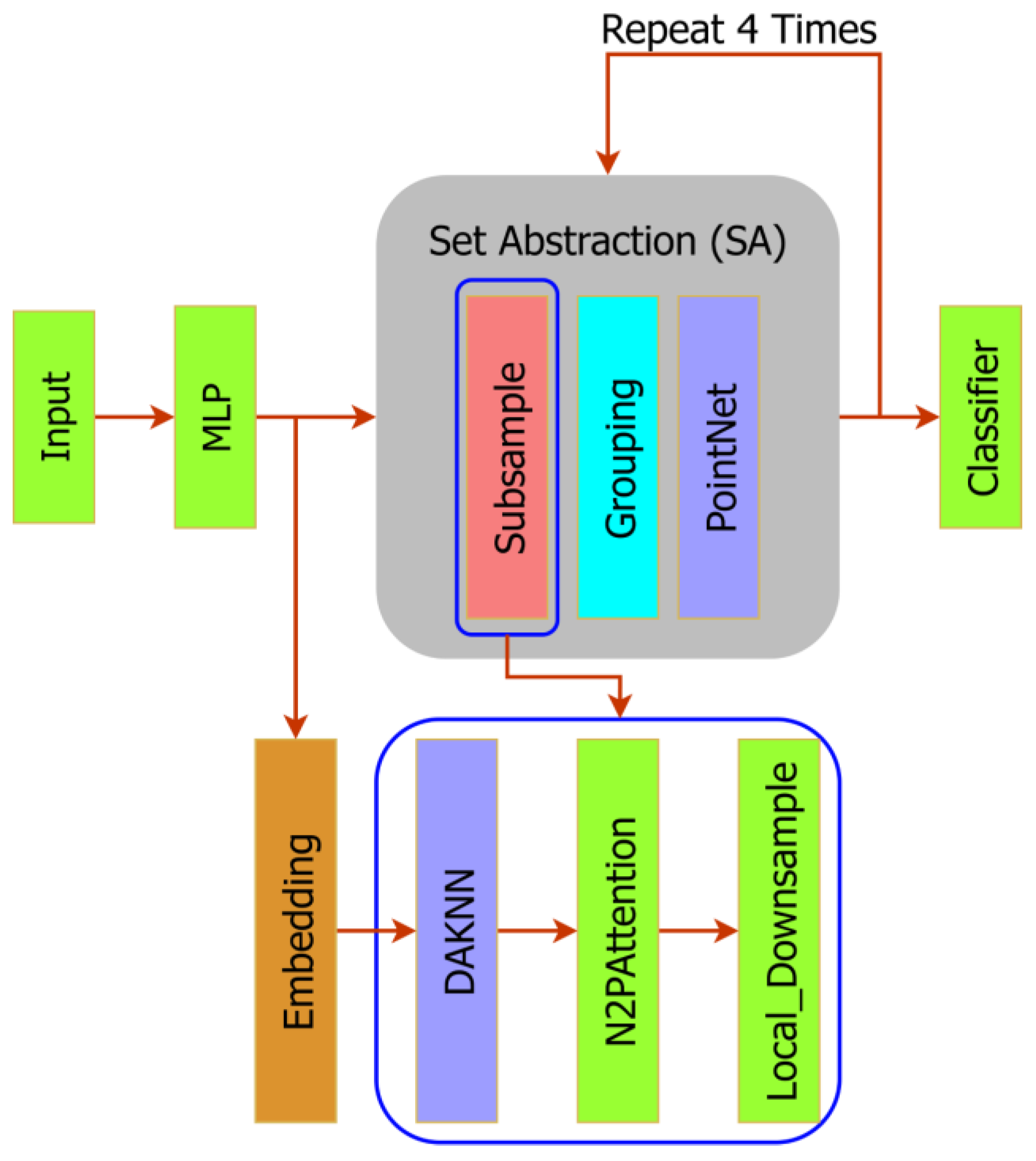
3.1. System Architecture

PointNext++ is an improved model based on PointNet. As shown in Figure 1, PointNeXt-S network architecture takes the input point cloud and elevates the dimensionality through an MLP layer. Then, it enters the set abstraction (SA) layer, which consists of a subsample layer, a grouping layer, and a PointNet layer, repeated four times. Finally, it passes through a classifier to output the result.

First, the batch size is set during input, which determines how many point cloud objects are trained simultaneously during each model update. Generally, a larger batch size improves generalization ability but also increases computational load and memory space requirements on the GPU. However, depending on the model complexity and optimizer used, a smaller batch size may sometimes yield better performance.

In this architecture, the input point cloud consists of 1024 points. In the ModelNet40 [28] dataset we used, each object originally had 2048 points. To enable the model to learn features more effectively during training and to reduce computational resources, it is common practice to downsample the 2048 points to a specified number through preprocessing before feeding them into the model. The decision to reduce the point cloud to 1024 points is based on previous experimental results from 3D point cloud classification models. The number 3 refers to the three channels of the point cloud, corresponding to the X, Y, and Z coordinates in the Cartesian coordinate system. To extract richer features, the MLP layer maps the point cloud to a higher dimension, allowing the subsequent grouping layer and PointNet layer in the SA layers to better capture feature information. After passing through the SA layer four times, it enters the classifier which includes the BN layer, ReLU, and Dropout, and finally outputs the result.

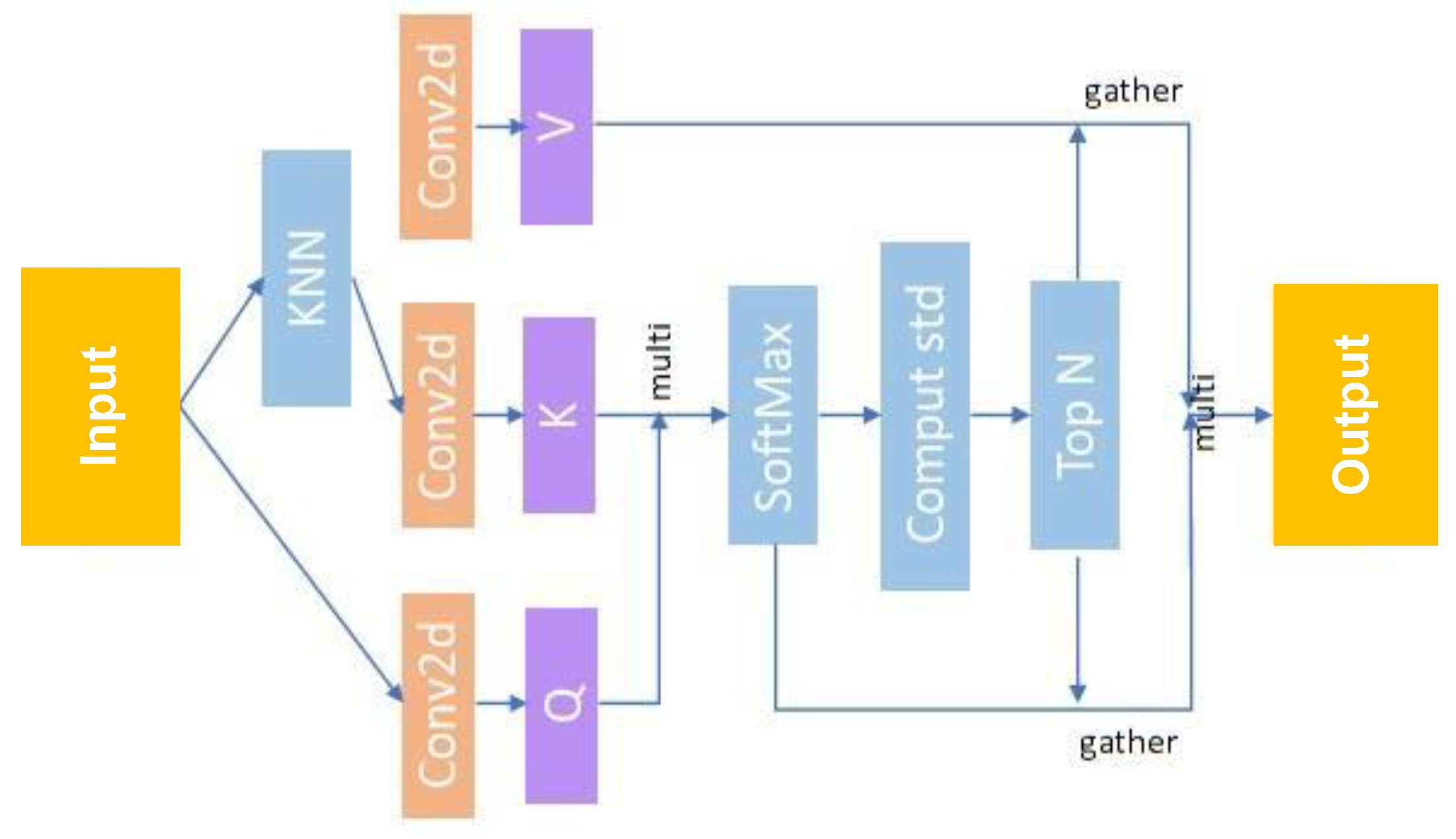
3.2. Attention-Based Point Cloud Edge Sampling

In the architecture of 3D point cloud classification networks, the overall data size of point clouds is large. If all point clouds are directly fed into the model, it would significantly increase the computational load and memory requirements. Therefore, subsampling point clouds is an indispensable step. Currently, models commonly use random sampling and farthest point sampling methods to address this issue.

The attention-based point cloud edge sampling (APES) [27] method revisits the Canny edge detection algorithm, discovering that when there is a large difference between a pixel or point set, the standard deviation increases. In other words, non-edge points have relatively average distances from their neighbors, resulting in smaller differences when calculating correlations. Conversely, edge points have significant differences in distances from their neighbors, leading to noticeable differences in correlation values. Thus, when searching for the same number of neighbors, the standard deviation for edge points is typically larger than for non-edge points. This method can determine the likelihood of a point being an edge point. Figure 2 illustrates the results of APES.

Compared to the farthest point sample (FPS) method, which aims for global coverage, the attention-based edge subsample method captures the overall contour of point cloud objects by obtaining edge points. Therefore, we replaced the subsample method in the PointNext-s network architecture with the attention-based edge subsample method to explore whether these two different subsample strategies affect the accuracy of 3D point cloud classification. In the APES method, we use a local subsample, and we conduct experiments using APES’s embedding layer and neighbors to point (N2P) attention layer.

3.2.1. Neighbor to Point (N2P) Attention Layer

To capture both local and global features in point cloud data, the APES method uses the N2P attention approach, which employs a multi-head self-attention mechanism to better understand and process complex point cloud data. As shown in Figure 3, the input point cloud is first grouped using the KNN method with a set neighborhood K value, obtaining the local neighborhood information for each point. The Query is generated through 2D convolutions and captures different features through multiple heads. The KNN grouping results are used to generate the Key and Value via 2D convolutions and are set for multi-head self-attention calculation. Next, the dot product between Query and Key is computed to obtain an energy matrix, which is then processed by the softmax function to derive attention weights. These weights are used to weight the Value matrix, resulting in a weighted feature representation. This representation is then combined with the original input features through a residual connection and normalized using a batch normalization layer to stabilize the model. Subsequently, further feature extraction is performed through fully connected layers, followed by another residual connection and batch normalization. This design effectively integrates local and global features, enhancing the network’s capability to process point cloud data.

3.2.2. Local Downsample Layer

Local downsample is a method that uses a self-attention mechanism through neighbors to subsample the input point cloud. As shown in Figure 4, in this method, the Query is generated through 2D convolution, while the Key and Value are obtained by grouping the input point cloud using the KNN method to get local neighborhoods. Each neighborhood has a predetermined number of neighbors K. After obtaining the local neighborhoods, 2D convolution is applied to understand the relationship and relative importance between the point cloud and its neighbors.

After completing the self-attention mechanism, the attention weights are obtained. These weights are used to calculate the standard deviation, which is then sorted by value. A larger standard deviation implies a higher likelihood of being an edge point. Finally, the required downsampled points are extracted in descending order of the standard deviation. This approach effectively reduces the number of points in the point cloud while retaining the edge features, thus achieving the goal of capturing the point cloud’s contour.

3.3. Density-Adaptive K Nearest Neighboring

In APES, the neighbor K value is set to 32. However, the density of each point in the point cloud objects varies. This means that in high-density areas, the K value can be appropriately reduced to decrease computational load while still obtaining useful feature information. Conversely, in low-density edge areas, a larger K value is needed to capture finer details.

We found a dynamic K value calculation method, density-adaptive k nearest neighboring (DAKNN), in the DA-Net [23]. The point cloud density d and the maximum density in the point cloud object are first obtained through kernel density estimation (KDE). To ensure that the appropriate K value is adaptively obtained in areas of different densities, d is taken as the reciprocal, and the scaling factor D is obtained through $D=d/\mathrm{m}\mathrm{a}\mathrm{x}\left(d\right)$. Next, the preliminary K value is calculated using $K_0=U\ast (N_0/N)$, where U is fixed at 32 based on the commonly used number of neighbors, $N_0$ is fixed at 1024, and N depends on the input point cloud. Finally, the final K value is obtained through $K=D\ast K_0$.

By calculating DAKNN and integrating it with the APES method, as shown in Figure 5, we can see that in the areas circled in yellow and green, the original APES method missed some edge points. However, with the adjustment using DAKNN, APES can capture finer details, resulting in more complete edge point contours. Figure 6 displays the effects on other point cloud objects: the left side shows the original point cloud in blue, the top right shows the results using only the APES method in red, and the bottom right shows the results after incorporating DAKNN. Our network architecture is illustrated in Figure 7. After elevating the features through the embedding layer, the K values are first calculated using DAKNN and then provided to the subsequent N2P attention for feature learning and local downsample for downsampling.

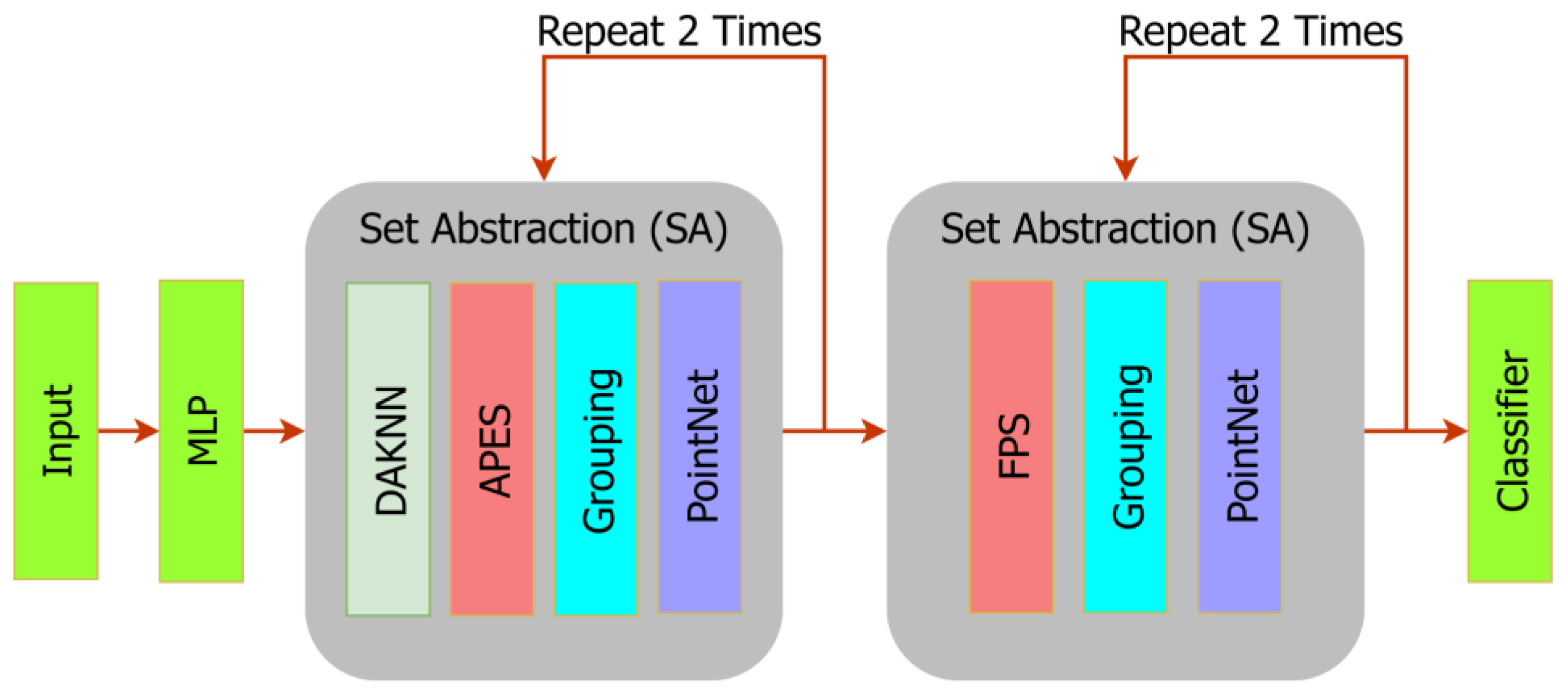
3.4. Network Architecture Adjustment

During our experiments, we found that combining the APES method with DAKNN improved the completeness of edge point capture, but did not significantly enhance accuracy. Upon observation, we noticed that during successive passes through four SA layers, the subsample feature points in the latter two layers gradually disappeared, as depicted in Figure 8. Taking a chair as an example in Figure 8, after passing through four SA layers consecutively, we observed that starting from the third SA layer, the contour of the chair back gradually vanished, leaving only the legs by the fourth layer. It is important to note that although the third layer in Figure 8 had 128 points clouds and the fourth layer had 64 points clouds, it does not necessarily mean that the APES method results in contour disappearance at 128 or 64 points. If, for instance, our SA layers downscaled from 256 points in the first pass, to 128 in the second, 64 in the third, and finally 32 points in the last layer, the APES subsample method could still capture contours fully at 128 points. However, the same issue persisted in the third and fourth layers.

To improve this situation, we adjusted the network architecture as shown in Figure 9. Initially, all four consecutive layers of the SA used the DAKNN and APES methods. We revised this so that the first two SA layers now utilize DAKNN and APES, while the latter two layers employ FPS for contour smoothing, ensuring more uniformity. After modifying the network architecture, we not only ensure the complete retention of edge points but also reduce computational overhead. The improved situation is depicted in Figure 10, where the third and fourth layers fully retain edge points using the FPS method.

4. Experiment

4.1. Dataset

We use ModelNet40 [28] as the training data for our experiments. ModelNet40 is a dataset for point cloud classification, created through CAD modeling and point cloud collection from models, so the point cloud data is noise-free and background-free, with each point cloud object representing a single object. It includes 40 categories, such as airplanes, beds, and chairs, with 9843 samples in the training set and 2468 samples in the test set. In addition to the original ModelNet40 dataset, there are two versions: one is modelnet40_ply_hdf5_2048, which reduces the original points to 2048 while retaining point coordinates and normals; the other is modelnet40_normal_resampled, which is a resampled and normalized version of ModelNet40 to reduce computational and memory requirements. We use the same data, modelnet40_ply_hdf5_2048, as PointNext for our experiments. Additionally, to enhance model learning capabilities, we preprocess the original 2048-point cloud data by downsampling it to 1024 points before training. The proportions of the training data set and test data set are 80% and 20%, respectively.

4.2. Experiment Platform

The experiment platform employed in this study is shown in

Table 1. Experiment platform specifications.

Experiment Platform
CPU	i7-13700 2.10 GHz
GPU	NVDIA GrForce RTX 4090
CPU Memory	32
GPU Memory	24
OS	Windows 11 (23.10.1)
Python Version	3.8.18
PyTorch Version	1.10.0
CUDA Runtime Version	11.8.89

.

4.3. Method Integration and Evaluation

In this section, we systematically integrated the methods used. In our experimental setup, as shown in

Table 2. Method integration and evaluation.

Methods	Input Points	K-Neighbor (Downsample)	Batch Size	Embedding Feature Size	Overall Accuracy	Average Accuracy
PointNext-s	1024	-	32	-	93.11%	89.96%
+Local_downsample	1024	32	32	-	91.17%	87.62%
+Embedding, Local_downsample	1024	32	32	128	92.42%	88.47%
+Embedding, Local_downsample, N2PAttention	1024	32	32	128	92.62%	89.36%
+Embedding, Local_downsample, N2PAttention, DAKNN	1024	8~32	32	128	93.23%	90.76%

, PointNext-s achieved an accuracy of 93.11%, which we used as our benchmark for comparison. By incorporating the DAKNN method, the experimental results not only improved accuracy by 0.6% compared to the APES method but also surpassed the original PointNext-s method. This indicates that using the DAKNN method alongside APES effectively enhances edge point detection, leading to an overall improvement in accuracy. The overall accuracy represents the correct classification rate of all points. Average accuracy is the average accuracy of each object.

4.4. Experiment in Kernel Density Estimation

In kernel density estimation, bandwidth is a smoothing parameter that significantly affects the results. Bandwidth acts as a scaling factor that primarily controls the width of the distribution among sample points. When the bandwidth is small, the sample points have a greater impact on the kernel density estimation, which can lead to overfitting and may not accurately reflect the true results. Conversely, when the bandwidth is large, it results in a smoother effect, but this excessive smoothing may overlook important features in the data. Therefore, the choice of bandwidth is crucial.

To effectively reduce the model’s training time, we used cross-validation in Python to calculate the optimal bandwidth for different point cloud objects after each stage of downsampling. The experimental results show that the average optimal bandwidth value is around 0.1. As shown in

Table 3. Experiment in kernel density estimation.

Methods	Input Points	BandWidth	Batch Size	Overall Accuracy	Average Accuracy
Ours	1024	0.05	32	93.07%	90.20%
	1024	0.1	32	93.23%	90.76%
	1024	0.15	32	93.15%	91.17%
	1024	0.2	32	93.07%	90.36%
	1024	0.25	32	93.03%	90.49%
	1024	0.3	32	93.15%	90.58%

, we initially set the bandwidth to 0.1 and conducted experiments within the range of 0.05 to 0.3 to adjust the required bandwidth. The experimental results indicate that a bandwidth of 0.1 yields the best results.

4.5. Subsample Using the APES and FPS Methods

After replacing the subsample methods with DAKNN and APES, we observed a slight improvement in accuracy, although not significant. In our network architecture, which includes four SA layers involving four subsample operations, we noticed through effect maps of each SA layer’s subsample that edge points gradually disappear in the last two layers. To ensure the retention of edge points and enable the latter SA layers to learn better features, we adopted DAKNN and APES for the first two SA layers and FPS for the last two layers. As shown in

Table 4. Subsample using the APES and FPS methods.

Methods	Input Points	Batch Size	SA Layers 1 and 2	SA Layers 3 and 4	Overall Accuracy	Average Accuracy
PointNext-s	1024	32	FPS	FPS	93.11%	89.96%
Ours	1024	32	APES	APES	92.38%	89.70%
	1024	32	DAKNN APES	DAKNN APES	93.23%	89.36%
	1024	32	DAKNN APES	FPS	93.35%	90.71%

, experimental results indicate that this combination of subsample methods not only preserves the point cloud contours effectively but also reduces computational time and improves accuracy.

4.6. Point Cloud Data Augmentation

In the PointNext paper, the importance of using different data augmentation methods for different datasets is discussed. According to their experimental results, translation and scaling are suitable data augmentation methods for the ModelNet40 dataset. Since this paper introduces an improved downsampling method, we conducted additional data augmentation experiments on top of the original data augmentation methods. As shown in

Table 5. Point cloud data augmentation.

Methods	Input Points	Batch Size	Overall Accuracy	Average Accuracy
PointCloud_Scale PointCloud_Translate	1024	32	93.35%	90.71%
PointCloud_Scale PointCloud_Translate +PointCloud_rotation	1024	32	93.44%	90.97%
PointCloud_Scale PointCloud_Translate +PointCloud_Jitter	1024	32	92.79%	90.16%
PointCloud_Scale PointCloud_Translate+ Random_Dropout (10%)	921	32	93.23%	90.92%

, we added point cloud rotation, jittering, and randomly dropping 10% of the points to the original translation and scaling. The experimental results show that point cloud rotation is effective for our method, improving the model’s accuracy. This differs from the findings in the PointNext paper, which mentioned that point cloud rotation did not have a significant effect on the ModelNet40 dataset. However, in our method, adding point cloud rotation as a data augmentation technique enhances the model’s performance.

This is because APES places more emphasis on selecting edge points during sampling. It calculates the standard deviation of each point to identify edge points. In contrast, PointNext uses FPS (farthest point sampling), which focuses on distributing the sampled points more evenly in space rather than specifically targeting edge points. The core idea behind data augmentation is that the semantics should remain unchanged after transformation. As long as the object’s outline remains intact, the semantics will not be altered regardless of rotation. However, in FPS, rotation can potentially cause semantic changes (e.g., after rotation, a point cloud of one object may become spatially similar to that of another object, resulting in similar point distributions). Therefore, by focusing on edge point sampling, APES can effectively use rotational data augmentation, enabling the model to learn invariance to these irrelevant changes and improving its generalization ability.

4.7. The Range of K Values for DAKNN

In the calculation of DAKNN, to prevent setting K values too small, we followed previous literature by setting the minimum value to 8, as shown in

Table 6. The range of K values for DAKNN.

Methods	Input Points	Max K	Min K	${\mathit{N}}_0$ Value	Batch Size	Overall Accuracy	Average Accuracy
Ours	1024	-	8	1024	32	93.25%	90.58%
	1024	32	8	512	32	93.44%	90.85%
	1024	24	8	512	32	93.23%	90.76%

. The experiments in this section were divided into three parts: the first part had no upper limit on K values, the second part set the maximum K value to 32, and the third part to 24. Experimental results indicated that setting the maximum K value to 32 yielded the best performance. Additionally, we found that adjusting N_0 in the original calculation formula, initially set at 1024, to match the number of points after the first subsample improved the model’s effectiveness. In our network architecture, where the initial subsample reduced the point cloud to 512 points, this adjustment also led to performance enhancements.

4.8. Final Experimental Results

In the previous experiments, we used hyperparameter settings based on the configuration from PointNext. However, since we changed the downsampling method, we adjusted the hyperparameters by referencing APES, and found that accuracy improved. Subsequently, we adjusted the batch size to 6 and observed a significant increase in accuracy.

We analyzed that this improvement might be due to the smaller batch size, which enhances model performance when using self-attention downsampling and calculating K values through DAKNN. As shown in

Table 7. Final experimental Results.

Methods	Input Points	Batch Size	Epochs	SA Layers 1 and 2	SA Layers 3 and 4	Overall Accuracy	Average Accuracy
PointNext-s	1024	32	600	FPS	FPS	93.11%	89.96%
	1024	6	200	FPS	FPS	92.54%	89.79%
+APES	1024	32	600	APES	APES	92.62%	89.36%
+DAKNN	1024	32	600	DAKNN APES	FPS	93.44%	90.85%
	1024	8	200	DAKNN APES	FPS	93.49%	90.70%
	1024	6	200	DAKNN APES	FPS	93.57%	91.14%

, we also applied the modified hyperparameters to the original PointNext-s model, where all four layers use farthest point sampling for downsampling. We found that the results of the original PointNext-s model declined. This suggests that different downsampling methods require different hyperparameter settings.

In the final experimental results, our method not only reduced the average training time by nearly 15% compared to PointNext-s, but also improved accuracy from 93.11% to 93.57%.

4.9. Comparison with Transformer-Based Architectures

We compare our method with state-of-the-art point cloud classification models based on Transformer architectures, including Point-BERT and Point Transformer. The core of Point Transformer lies in its use of vector self-attention within local regions, combined with a learnable position encoding. This design effectively captures both local and global relationships.

Point-BERT, on the other hand, segments point clouds into local regions and encodes them into discrete codes using a discrete variational autoencoder (dVAE). It then performs self-supervised pretraining through masked point modeling (MPM), where the model learns to reconstruct local geometric structures from partially masked inputs. This approach effectively captures both local and global features of point clouds, significantly improving performance in classification and few-shot learning tasks, and shows strong transferability.

The

Table 8. Comparison with Transformer-based architectures.

Method	Architectures	Input Point	Overall Acc.
Point Transformer	Transformer	-	93.70%
[ST] Point-BERT (1k)	Transformer-based	1024	93.20%
[ST] Point-BERT (8k)	Transformer-based	8192	93.80%
PointNext-s + APES + DAKNN	CNN + DAKNN/APES	1024	93.57%

below shows the classification results on the ModelNet40 dataset. Point-BERT achieves the highest overall accuracy of 93.8% when using 8k points. However, with only 1024 points, our model already achieves 93.57% accuracy, nearly on par. Even compared to Point Transformer, our model is only 0.13% lower in accuracy. Despite this, Point Transformer uses 4.9 million parameters, while our model uses only 4.5231 million, reducing the parameter count by nearly 400,000.

4.10. Comparison of Time at Different K Values

According to

Table 9. Comparison of time at different K values.

K Value	Epoch	Time	Accuracy
8	600	08:14:58	OA: 92.63  mAcc: 90.15
	300	04:05:24	OA: 92.79   mAcc: 90.13
16	300	04:18:08	OA: 92.67   mAcc: 90.35
32	300	04:49:58	OA: 92.71   mAcc: 89.90
	600	10:05:54	OA: 92.38   mAcc: 89.54
Adaptive (8~32)	300	05:25:30	OA: 92.91   mAcc: 90.12
	600	10:55:54	OA: 92.50   mAcc: 89.30
Adaptive (8~16)	300	05:14:27	OA: 92.63   mAcc: 90.43

, although the accuracy of the adaptive K method in the original paper is not significantly different from that of using a fixed K value, the support of adaptive K makes the model overall more stable and achieves the highest accuracy. However, the computational time remains non-negligible.

Table 10. The percentage increase in calculation time for different K values.

Epoch	K Value
	Adaptive	8	16	32
300	5.3 h	4.10 h	4.30 h	4.80 h
600	10.9 h	8.25 h	-	10.10 h

. shows the percentage increase in computation time for different K values.

4.11. Adaptive Kernel Density Experiment

We experimented with adaptive kernel density estimation (adaptive KDE) [29], whereas the original paper used standard KDE. Adaptive KDE selects a different bandwidth for each data point, adjusting automatically based on the local data density. In denser regions, a smaller bandwidth is used (for higher resolution), while in sparser regions, a larger bandwidth is applied (to avoid overfitting). This method captures sharp variations in data distribution more effectively, but it comes with a higher computational cost.

Based on the current experimental results (

Table 11. Adaptive kernel density experiment.

Bandwidth	Epoch	Time	Accuracy
0.1	200	-	OA: 92.63  mAcc: 90.30
	600	10:55:54	OA: 92.50   mAcc: 89.30
Adaptive (0.1~0.2)	200	03:42:08	OA: 92.59   mAcc: 90.50
	600	11:01:28	OA: 92.18   mAcc: 90.12
Adaptive (0.12~0.17)	200	03:54:54	OA: 92.59   mAcc: 89.44

), it can be observed that the adaptive bandwidth has almost no impact compared to the original method.

We conducted two types of noise tests on ModelNet40 to evaluate the model’s generalization and robustness under unseen disturbances. First, we performed outlier and noise injection experiments by randomly adding noise points (ranging from 1% to 20% of the original point cloud) to simulate real-world interference. Results showed that when noise was below 19%, the overall accuracy (OA) remained nearly unchanged, and even at 20% noise, the OA only slightly decreased, staying above 92%. With adversarial training, the model maintained its performance even under 20% noise, demonstrating strong robustness. This is largely attributed to the N2P sampling mechanism in APES, which uses a self-attention-based relation graph to assess the relevance between each point and its neighbors. Since outliers have low relational scores due to distant neighbors, they are unlikely to be sampled, effectively reducing the impact of noise.

Next, we simulated point cloud shift scenarios by randomly offsetting 1% to 10% of the points with varying magnitudes (from 0.01 to 0.1) to test the model’s sensitivity to geometric disturbances. The results showed that when the offset magnitude was below 0.06, each 0.01 increase led to only a minor drop in OA. Even with 10% of points being shifted, the model maintained over 90% OA as long as the offset was under 0.3. However, when the shift became larger, accuracy dropped significantly, likely due to the disruption of the point cloud structure, which altered edge point locations and neighborhood relationships, thus weakening the model’s recognition ability.

For the offset test, we compare primarily against our original noise results (OA: 92.91, mAcc: 90.12). Results with OA ≥ 92 and mAcc ≥ 89 are highlighted in red text. The yellow background indicates the red-text result with the highest noise ratio. The detailed results are shown in

Table 12. Compare the results after offset noise (original results: OA: 92.91, mAcc: 90.12).

Noise Ratio		Offset
		0.01	0.02	0.03	0.04	0.05	0.06	0.07	0.08	0.09	0.10
1%	OA	93.03	92.46	92.87	92.42	92.26	92.30	92.26	92.22	92.50	92.54
	mAcc	90.60	89.04	90.00	89.30	89.40	89.20	89.03	89.63	90.03	89.59
2%	OA	92.50	92.10	92.26	92.26	92.14	91.25	91.09	91.21	91.45	91.33
	mAcc	89.87	89.37	89.82	89.40	89.53	88.47	88.24	87.95	88.72	88.41
4%	OA	92.46	92.26	92.06	91.61	91.17	91.29	90.68	89.71	89.34	89.30
	mAcc	89.82	89.28	89.29	88.69	87.93	88.05	86.93	87.06	85.79	85.06
7%	OA	92.30	92.10	91.37	90.92	90.19	89.87	88.37	87.52	86.26	85.05
	mAcc	89.14	89.28	88.00	87.60	85.95	85.64	83.96	81.86	81.90	79.00
10%	OA	92.59	91.73	90.92	89.99	88.98	87.88	86.51	84.24	82.09	79.54
	mAcc	89.81	88.92	87.60	85.85	83.80	83.33	80.06	78.06	74.20	71.91

. Due to space limitations, we have removed some results from Table 12.

For the noise experiments, we introduced noise by randomly adding 1% to 20% noisy points. Models were trained using data with 5%, 10%, 15%, and 20% noise levels, and tested on data with noise levels ranging from 0% to 20%. The general results are shown below. The “average” refers to the mean performance across all noise levels from 1% to 20%. Due to space limitations, we only present the results for 0%, 5%, 10%, 15%, and 20% in

Table 13. Compare the results after adding noise (original results: OA: 92.91, mAcc: 90.12).

Testing SNR		Training SNR
		0%	5%	10%	15%	20%
0%	OA	92.71	93.23	93.15	93.11	92.87
	mAcc	89.90	90.84	90.29	91.01	90.09
5%	OA	92.14	92.95	93.64	93.19	92.38
	mAcc	89.52	90.51	90.72	90.90	89.86
10%	OA	92.83	92.83	93.31	93.07	92.91
	mAcc	90.17	89.58	90.49	90.87	90.05
15%	OA	92.75	92.54	92.59	93.27	93.27
	mAcc	90.49	90.05	89.23	90.73	90.75
20%	OA	91.98	92.63	93.07	92.38	92.59
	mAcc	89.86	89.80	90.03	89.76	89.90
Avg.	OA	92.55	92.88	93.00	92.97	92.77
	mAcc	90.11	90.12	90.02	90.51	90.29

.

5. Conclusions

We modified the downsampling method in the PointNext network architecture to the self-attention-based edge downsampling method, APES, and used DAKNN’s adaptive K approach to make the edge points obtained by APES more complete. In the original four consecutive SA layers, we found that with APES, the point cloud’s contour gradually disappeared in the downsampling results of the third and fourth layers. To address this issue, we used DAKNN and APES in the first two SA layers to obtain the edge points of the point cloud, while using FPS in the last two SA layers to preserve the contour of the downsampled point cloud.

After integrating different data augmentation methods and adjusting the hyperparameters, our average accuracy on the ModelNet40 dataset improved by 0.46%, from 93.11% to 93.57%, compared to the original PointNext-s method. Our main contributions can be summarized in the following three points:

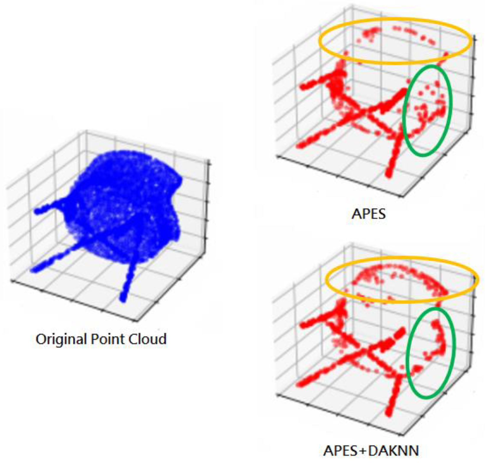
• By using the DAKNN approach to calculate the K value, the original APES downsampling method better captures the edge points of the point cloud, making the contours more complete.
• The combination of two downsampling methods, along with effective data augmentation techniques, enhances computational efficiency and effectively improves accuracy.
• In addition to changing the original PointNext-s downsampling method, we also adjusted the hyperparameters. As a result, our method not only successfully improved accuracy but also reduced the model’s average training time by approximately 15% compared to the original PointNext-s.

Downsampling methods are indispensable in many current point cloud classification models. Therefore, further considering the relationships between points in downsampling methods and capturing useful feature information to enhance feature learning during network training could be a future direction for improving accuracy in point cloud classification models.

References

1. Qi, C.R.; Su, H.; Mo, K.; Guibas, L.J. Pointnet: Deep learning on point sets for 3d classification and segmentation. In Proceedings of the IEEE Conference on Computer Vision and Pattern Recognition, Honolulu, HI, USA, 21–26 July 2017. [Google Scholar]
2. Qi, C.R.; Yi, L.; Su, H.; Guibas, L.J. Pointnet++: Deep hierarchical feature learning on point sets in a metric space. Adv. Neural Inf. Process. Syst. 2017, 30, 5105–5114. [Google Scholar]
3. Ma, X.; Qin, C.; You, H.; Ran, H.; Fu, Y. Rethinking network design and local geometry in point cloud: A simple residual MLP framework. arXiv 2022, arXiv:2202.07123. [Google Scholar]
4. Qian, G.; Li, Y.; Peng, H.; Mai, J.; Hammoud, H.; Elhoseiny, M.; Ghanem, B. Pointnext: Revisiting pointnet++ with improved training and scaling strategies. Adv. Neural Inf. Process. Syst. 2022, 35, 23192–23204. [Google Scholar]
5. Guo, Y.; Wang, H.; Hu, Q.; Liu, H.; Liu, L.; Bennamoun, M. Deep learning for 3d point clouds: A survey. IEEE Trans. Pattern Anal. Mach. Intell. 2020, 43, 4338–4364. [Google Scholar] [CrossRef] [PubMed]
6. Mirbauer, M.; Krabec, M.; Křivánek, J.; Šikudová, E. Survey and evaluation of neural 3d shape classification approaches. IEEE Trans. Pattern Anal. Mach. Intell. 2021, 44, 8635–8656. [Google Scholar] [CrossRef]
7. Camuffo, E.; Mari, D.; Milani, S. Recent advancements in learning algorithms for point clouds: An updated overview. Sensors 2022, 22, 1357. [Google Scholar] [CrossRef]
8. Zhang, H.; Wang, C.; Tian, S.; Lu, B.; Zhang, L.; Ning, X.; Bai, X. Deep learning-based 3D point cloud classification: A systematic survey and outlook. Displays 2023, 79, 102456. [Google Scholar] [CrossRef]
9. Kyaw, P.P.; Tin, P.; Aikawa, M.; Kobayashi, I.; Zin, T.T. Cow’s Back Surface Segmentation of Point-Cloud Image Using PointNet++ for Individual Identification. In Genetic and Evolution-Ary Computing; Pan, J.S., Zin, T.T., Sung, T.W., Lin, J.C.W., Eds.; Springer: Singapore, 2025; Volume 1321. [Google Scholar] [CrossRef]
10. Li, J.; Chen, B.M.; Lee, G.H. So-net: Self-organizing network for point cloud analysis. In Proceedings of the IEEE Conference on Computer Vision And Pattern Recognition, Salt Lake City, UT, USA, 18–23 June 2018. [Google Scholar]
11. Zhao, H.; Jiang, L.; Fu, C.-W.; Jia, J. Pointweb: Enhancing local neighborhood features for point cloud processing. In Proceedings of the IEEE/CVF Conference on Computer Vision and Pattern Recognition, Long Beach, CA, USA, 15–20 June 2019. [Google Scholar]
12. Hu, Q.; Yang, B.; Xie, L.; Rosa, S.; Guo, Y.; Wang, Z.; Trigoni, N.; Markham, A. Randla-net: Efficient semantic segmentation of large-scale point clouds. In Proceedings of the IEEE/CVF Conference on Computer Vision and Pattern Recognition, Seattle, WA, USA, 13–19 June 2020. [Google Scholar]
13. Xu, M.; Zhang, J.; Zhou, Z.; Xu, M.; Qi, X.; Qiao, Y. Learning geometry-disentangled representation for complementary understanding of 3d object point cloud. In Proceedings of the AAAI Conference on Artificial Intelligence, Long Beach, CA, USA, 15–20 June 2019. [Google Scholar]
14. Vaswani, A.; Shazeer, N.; Parmar, N.; Uszkoreit, J.; Jones, L.; Gomez, A.N.; Kaiser, Ł.; Polosukhin, I. Attention is all you need. Adv. Neural Inf. Process. Syst. 2017, 30, 5998–6008. [Google Scholar]
15. Guo, M.-H.; Cai, J.-X.; Liu, Z.-N.; Mu, T.-J.; Martin, R.R.; Hu, S.-M. Pct: Point cloud transformer. Comput. Vis. Media 2021, 7, 187–199. [Google Scholar] [CrossRef]
16. Zhao, H.; Jiang, L.; Jia, J.; Torr, P.H.; Koltun, V. Point transformer. In Proceedings of the IEEE/CVF International Conference on Computer Vision, Montreal, BC, Canada, 11–17 October 2021. [Google Scholar]
17. Devlin, J.; Chang, M.-W.; Lee, K.; Toutanova, K. Bert: Pre-training of deep bidirectional transformers for language understanding. arXiv 2018, arXiv:1810.04805. [Google Scholar]
18. Yu, X.; Tang, L.; Rao, Y.; Huang, T.; Zhou, J.; Lu, J. Point-bert: Pre-training 3d point cloud transformers with masked point modeling. In Proceedings of the IEEE/CVF Conference on Computer Vision and Pattern Recognition, New Orleans, LA, USA, 18–24 June 2022. [Google Scholar]
19. Berg, A.; Oskarsson, M.; O’Connor, M. Points to patches: Enabling the use of self-attention for 3d shape recognition. In Proceedings of the 2022 26th International Conference on Pattern Recognition (ICPR), Montreal, QC, Canada, 21–25 August 2022. [Google Scholar]
20. Tao, W.; Chen, H.; Moniruzzaman, M.; Leu, M.C.; Yi, Z.; Qin, R. Attention-Based Sensor Fusion for Human Activity Recognition Using IMU Signals. arXiv 2021, arXiv:2112.11224. [Google Scholar]
21. Dovrat, O.; Lang, I.; Avidan, S. Learning to sample. In Proceedings of the IEEE/CVF Conference on Computer Vision and Pattern Recognition, Long Beach, CA, USA, 15–19 June 2019. [Google Scholar]
22. Lang, I.; Manor, A.; Avidan, S. Samplenet: Differentiable point cloud sampling. In Proceedings of the IEEE/CVF Conference on Computer Vision and Pattern Recognition, Seattle, WA, USA, 13–19 June 2020. [Google Scholar]
23. Lin, Y.; Huang, Y.; Zhou, S.; Jiang, M.; Wang, T.; Lei, Y. DA-Net: Density-adaptive downsampling network for point cloud classification via end-to-end learning. In Proceedings of the 2021 4th International Conference on Pattern Recognition and Artificial Intelligence (PRAI), Yibin, China, 20–22 August 2021. [Google Scholar]
24. Qian, Y.; Hou, J.; Zhang, Q.; Zeng, Y.; Kwong, S.; He, Y. Mops-net: A matrix optimization-driven network fortask-oriented 3d point cloud downsampling. arXiv 2020, arXiv:2005.00383. [Google Scholar]
25. Wang, X.; Jin, Y.; Cen, Y.; Lang, C.; Li, Y. Pst-net: Point cloud sampling via point-based transformer. In Proceedings of the Image and Graphics: 11th International Conference, ICIG 2021, Haikou, China, 6–8 August 2021; Springer: New York, NY, USA, 2021. [Google Scholar]
26. Wang, X.; Jin, Y.; Cen, Y.; Wang, T.; Tang, B.; Li, Y. Lightn: Light-weight transformer network for performance-overhead tradeoff in point cloud downsampling. IEEE Trans. Multimed. 2023, 27, 832–847. [Google Scholar] [CrossRef]
27. Wu, C.; Zheng, J.; Pfrommer, J.; Beyerer, J. Attention-based Point Cloud Edge Sampling. In Proceedings of the IEEE/CVF Conference on Computer Vision and Pattern Recognition, Vancouver, BC, Canada, 17–24 June 2023. [Google Scholar]
28. Wu, Z.; Song, S.; Khosla, A.; Yu, F.; Zhang, L.; Tang, X.; Xiao, J. 3d shapenets: A deep representation for volumetric shapes. In Proceedings of the IEEE Conference on Computer Vision and Pattern Recognition, Boston, MA, USA, 7–12 June 2015. [Google Scholar]
29. Wang, L.; Chen, Y.; Song, W.; Xu, H. Point Cloud Denoising and Feature Preservation: An Adaptive Kernel Approach Based on Local Density and Global Statistics. Sensors 2024, 24, 1718. [Google Scholar] [CrossRef]
Figure 1. The architecture of the PointNext-s.
Electronics 14 02439 g001
Figure 2. The downsampling effect of APES.
Electronics 14 02439 g002
Figure 3. The flowchart of N2P attention layer.
Electronics 14 02439 g003
Figure 4. The flowchart of local downsample layer.
Electronics 14 02439 g004
Figure 5. Comparison chart after adding the DAKNN method.
Electronics 14 02439 g005
Figure 6. Comparison of point cloud objects after adding the DAKNN method.
Electronics 14 02439 g006
Figure 7. The architecture of the network.
Electronics 14 02439 g007
Figure 8. Edge points disappear in SA layers 3 and 4.
Electronics 14 02439 g008
Figure 9. The architecture of the network uses the DAKNN and APES method for SA layers 1 and 2, and the FPS method for SA layers 3 and 4.
Electronics 14 02439 g009
Figure 10. Effect diagram of SA layers 3 and 4 using FPS.
Electronics 14 02439 g010