Rain Noise Cancellation Technique for LiDAR System Using Convolutional Neural Network

Abstract

LiDAR is a technology that uses laser pulses to measure an object’s distance, an essential technology for Advanced Driver Assistance Systems (ADASs). However, it can be affected by adverse weather environments that may reduce the safety of ADASs. This paper proposes a convolutional neural network that utilizes lightweight network nodes with multiple repetitions instead of the traditional large-scale model. The proposed approach reduces the parameter size, and a consistent pre-processing method is designed to control the input parameters of the network. This process reduces the data size while retaining sufficient features for neural network training. The method was tested on a LiDAR system, demonstrating its ability to run on simple embedded systems and be deployed in heavy rain environments for real-time processing. The proposed convolutional neural Repetitive Lightweight Feature-preserving Network (RLFN) for LiDAR noise filtering demonstrates significant potential for generalization across various adverse weather conditions and environments. This paper discusses the theoretical and practical aspects of the model’s generalization capabilities. By theoretical justification, the design of our model incorporates several key features that enhance its ability to generalize: (1) Adaptive pre-processing—The adaptive pre-processing method standardizes input sizes while preserving essential features. This ensures that the model can handle varying data distributions and noise patterns, making it robust to different types of adverse weather conditions. (2) Inception and residual structures—The use of inception modules and residual connections allows the model to capture multi-scale features and maintain gradient flow, respectively. These structures are known for their robustness and ability to generalize well across different tasks and datasets. (3) Lightweight network design: The lightweight nature of the network, combined with repetitive loops, ensures efficient computation without sacrificing performance. This design is particularly beneficial for deployment on embedded systems, which often have limited computational resources. As verified by testing on a dataset, WADS, the RLFN demonstrated 98.53% accuracy, with a 96.31% F1 score.

1. Introduction

LIDAR is a commonly used sensor in automated driving systems for multi-environment detection and vehicle localization [1,2]. However, its working principle limits its resolution [3]. Therefore, it is often used with a camera to enhance object recognition capability. Using multiple sensors, including LiDAR, can improve system reliability, ensuring safe and smooth operation while avoiding collisions.

Although LiDAR has benefits, adverse weather conditions can affect its performance. This can cause the sensor to generate large amounts of erroneous data, leading to misjudgments by the autonomous driving system. Heavy rain, snow, and fog can cause the laser beam to reflect or scatter prematurely, resulting in misjudgment by the sensor and a reduction in its operating range and reliability. Figure 1 illustrates the interference with LiDAR in heavy rain/snow conditions.

LiDAR captures numerous snow spots around the vehicle, significantly limiting the sensor’s field of view and causing interference with the automated driving system. Filtering the LiDAR point cloud to remove noise points is necessary to improve the reliability of the automatic driving system. This is significant for enhancing the safety of automatic driving.

The use of sensors, including optical sensors, has increased in various applications, such as autonomous vehicles. As a result, noise filtering has become a crucial aspect to improve the accuracy of target detection and recognition. In recent years, several noise filters have been developed to enhance the performance of autonomous vehicles under extreme weather conditions [2,3,4,5]. Advanced machine learning techniques are used by these filters to detect and remove noise from sensor data [6], while others use methods that improve hardware or signal processing techniques to achieve similar results [7,8,9].

Advanced noise filtering techniques are necessary for LiDAR point cloud data as conventional filters are less efficient. While conventional filters have shown impressive results in removing noise points, they also eliminate points belonging to real objects, resulting in the loss of valuable information from the LiDAR data.

Reducing algorithm hardware requirements is necessary due to the high cost of hardware. Lower hardware requirements enable deployment on less expensive platforms, widening the range of applications.

In this research, specific innovations are highlighted as follows: (1) Adaptive Pre-Processing Method—We emphasize the adaptive pre-processing method, which standardizes input sizes while preserving essential features, which might not be common in existing methods. (2) Combination of Techniques—While inception modules, residual connections, and lightweight structures are well-known, the specific combination and application to LiDAR noise filtering in adverse weather conditions might be unique. Our recursive process for making the combination improves performance. (3) Real-Time Processing on Embedded Systems—Our method has the ability to run efficiently on simple embedded systems, which is crucial for real-time applications in autonomous driving. (4) Performance Metrics—Based on its superior performance metrics (accuracy, precision, recall, F1 score), our method achieved improvements compared to existing techniques like WeatherNet and conventional filters.

2. Related Works

LiDAR is a dependable sensor for autonomous vehicles, but its performance can be affected by certain weather conditions. Visibility and noise pose significant challenges for LiDAR in adverse weather conditions. Heavy rain, snow, or fog can scatter the laser beam, leading to reduced sensor range or inaccurate readings [9,10,11,12,13]. In extreme cases, the sensor may fail to detect any object at all. LiDAR sensors currently have limitations in adverse weather conditions. Various methods have been proposed to address this issue to mitigate the noise generated by bad weather. Conventional techniques for optical point cloud noise filtering include the ROR (radius outlier removal) and SOR (statistical outlier removal) algorithms [14,15]. These algorithms identify and remove data points that deviate significantly from most of the data, thereby reducing errors and noise in the point cloud. These methods classify noise based on the clustering of point clouds, distinguishing them from dense clusters that represent actual objects. Conventional filters may offer advantages in terms of speed, but they may have limitations in terms of accuracy and reliability. Additionally, their construction is usually simple and does not consider the object data’s density variations.

Several adaptive filters have been proposed to address the limitations of conventional methods, including dynamic statistical outlier removal (DSOR) [16], dynamic radius outlier removal (DROR) [17], and low-intensity outlier (LIOR) [18]. DROR and DSOR adjust the search radius based on the distance between the object and the LiDAR sensor. DSOR dynamically changes the average distance based on the distance of each point in the LiDAR data. To improve the effectiveness of the filters, it is essential to consider that the object point cloud density decreases with increasing distance from LiDAR. The search radius is defined as the product of the multiplicative constant and the object distance. The effectiveness of these adaptive filters is demonstrated by the results of DROR and DSOR, which achieve more than 90% accuracy in preserving the details of the LiDAR point cloud without removing environmental features. These advances highlight the potential of adaptive filtering to improve the quality and reliability of LiDAR point cloud segmentation and analysis. On the other hand, LIOR adds a reflective intensity filter to ROR. This is because the intensity of a noise point is usually lower than that of the target point at the same distance. Therefore, LIOR first filters out most of the noise points using the intensity filter and then applies the ROR algorithm.

Another class of approaches uses deep learning to filter out adverse weather effects in point cloud data through CNN-based methods, providing an opportunity to address the challenge of noise removal from LiDAR data [19]. These models can potentially improve the accuracy and reliability of sensor data, impacting fields such as self-driving cars, robotics, and healthcare. Studies investigate using computer vision techniques to classify noise in LiDAR data by converting it into image formats [20]. The resulting images are then utilized to train models capable of recognizing and classifying noise features. An example of this approach is WeatherNet [21], which reduces the network’s depth because the noise-filtering task has fewer classes. The model employs an inception layer with a dilated convolution to handle various inputs and expand the receptive field. Additionally, a dropout layer is incorporated to enhance generalization. GPUs can perform deep learning techniques, which are significantly more efficient than CPUs.

Current filters have low target retention due to a significant gap between accuracy and recall. To overcome this limitation, a new approach based on deep learning networks is proposed in this study. A consistent pre-processing method is designed to control the input parameters of the network at the same size. This is achieved by creating a lightweight neural network and including laser ID as an additional input parameter. The proposed approach significantly improves WADS dataset, with F1 scores exceeding 95%. The proposed filter effectively removes noise points while preserving object points, which is crucial for the accurate operation of the automated driving system. Additionally, the small size of the filter reduces hardware requirements and optimizes system execution time, improving overall efficiency.

Zhao et al. [22] present a multi-task learning (MTL) framework to perform simultaneous point-wise segmentation, ground removal, and outlier filtering in real time for LiDAR perception pipelines. The key innovation lies in its shared encoder–decoder structure, where task-specific decoders allow the network to adaptively refine representations based on each objective. This method achieves competitive performance with low latency and is optimized for deployment in autonomous vehicles. The concept of task integration is relevant to our approach, as we similarly aim to reduce computational overhead in embedded systems.

Zhang et al. [23] propose a lightweight attention-based neural network for efficient 3D point cloud registration. Their approach replaces heavy transformer encoders with point-wise attention blocks, reducing memory usage while maintaining high registration accuracy. The work is particularly significant for applications requiring on-board SLAM and localization under resource constraints. While their application domain differs, the architectural philosophy—favoring compact design and feature-level attention—is aligned with our motivation to minimize parameters while retaining performance in LiDAR denoising.

Tsai and Peng [24] introduce a probabilistic ground segmentation algorithm designed to handle dense snowfall and rainfall in SLAM applications. Unlike deterministic filters, their method dynamically adjusts segmentation thresholds based on estimated local point cloud density distributions, improving robustness in noisy environments. Their research contributes to the broader field of LiDAR noise handling and complements our focus by addressing the segmentation side of the problem, whereas we target point-wise noise identification and filtering.

The above recent advances further emphasize the need for lightweight, robust LiDAR pre-processing under environmental constraints. For instance, Zhao et al. [22] proposed a real-time multi-task learning model to jointly address segmentation, ground removal, and outlier detection, highlighting the advantages of shared task representations for embedded systems. Zhang et al. [23] introduced a compact attention mechanism for 3D registration, which mirrors our design philosophy of low-parameter architectures for point cloud processing. Moreover, Tsai & Peng [24] developed an adaptive ground segmentation technique based on probabilistic density thresholds, enhancing SLAM performance in heavy precipitation scenarios. These works reinforce the growing importance of efficient, weather-resilient LiDAR models, supporting the direction and necessity of our proposed RLFN.

3. The Proposed Method

This chapter introduces an adaptive pre-processing method based on variable range thresholds to process inputs of different sizes into same-sized outputs while preserving the desired features. The processed data can be easily restored to the original data. Additionally, a neural network is proposed that incorporates inception, residual, and parallel structures to improve the data generated by LiDAR under adverse weather conditions.

3.1. Pre-Processing

Due to the characteristics of neural networks, if the batch size is larger than 1, the input size must be the same. Therefore, there are usually two ways to handle this situation: padding the point cloud to the same size or reducing the data to the same size.

Filling the data is an option to maintain the original features and avoid unnecessary additions. However, this method increases the data size and hardware requirements. Alternatively, padding the data should be avoided as it introduces unnecessary features. Therefore, the data reduction method was chosen.

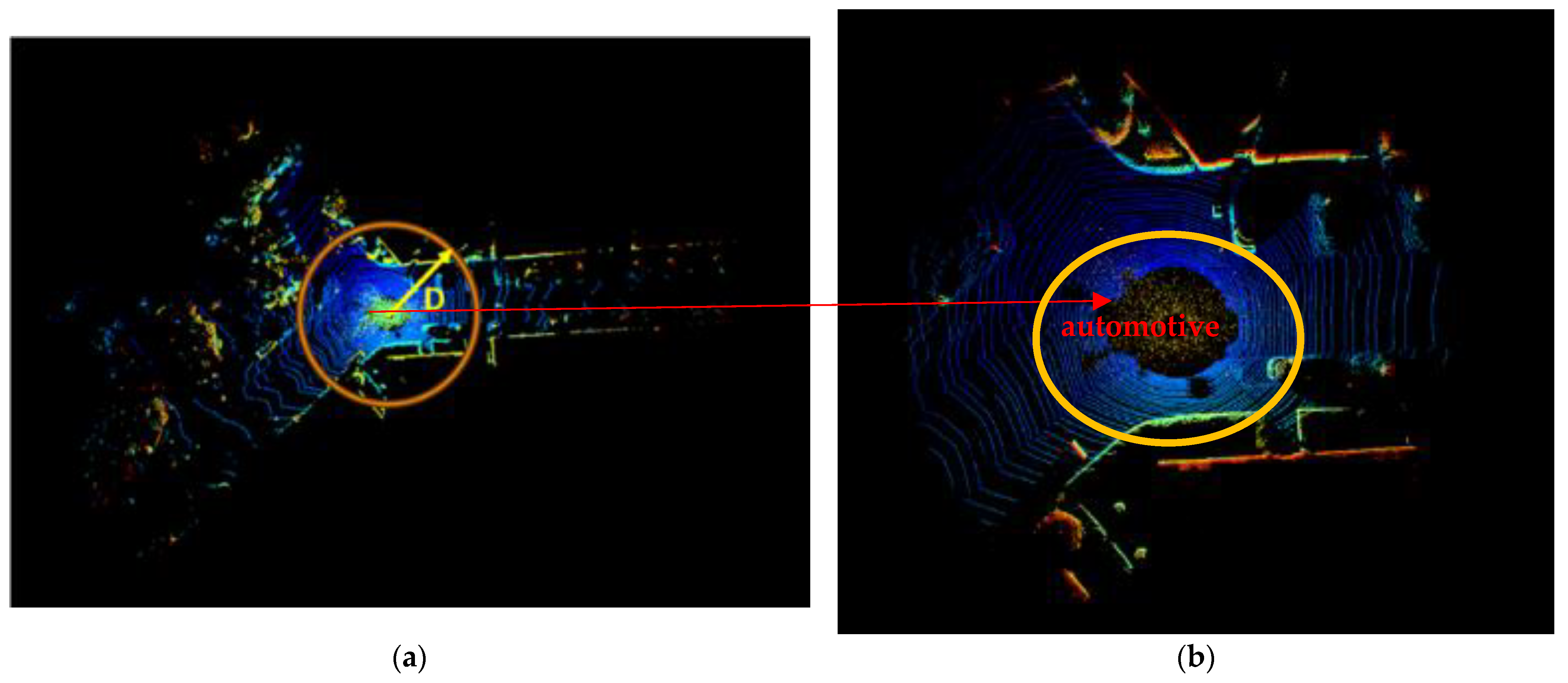
An adaptive algorithm is proposed in this study, as illustrated in Figure 2a. The algorithm begins by creating a circle with a radius D centered at the origin. The size of D is automatically adjusted to ensure that the number of points in the circle is consistent for each frame’s point cloud. Based on the examination of various datasets, as depicted in Figure 2b, it is evident that noise points generated in adverse weather conditions are concentrated around LiDAR, with no noise points observed beyond a distance D.

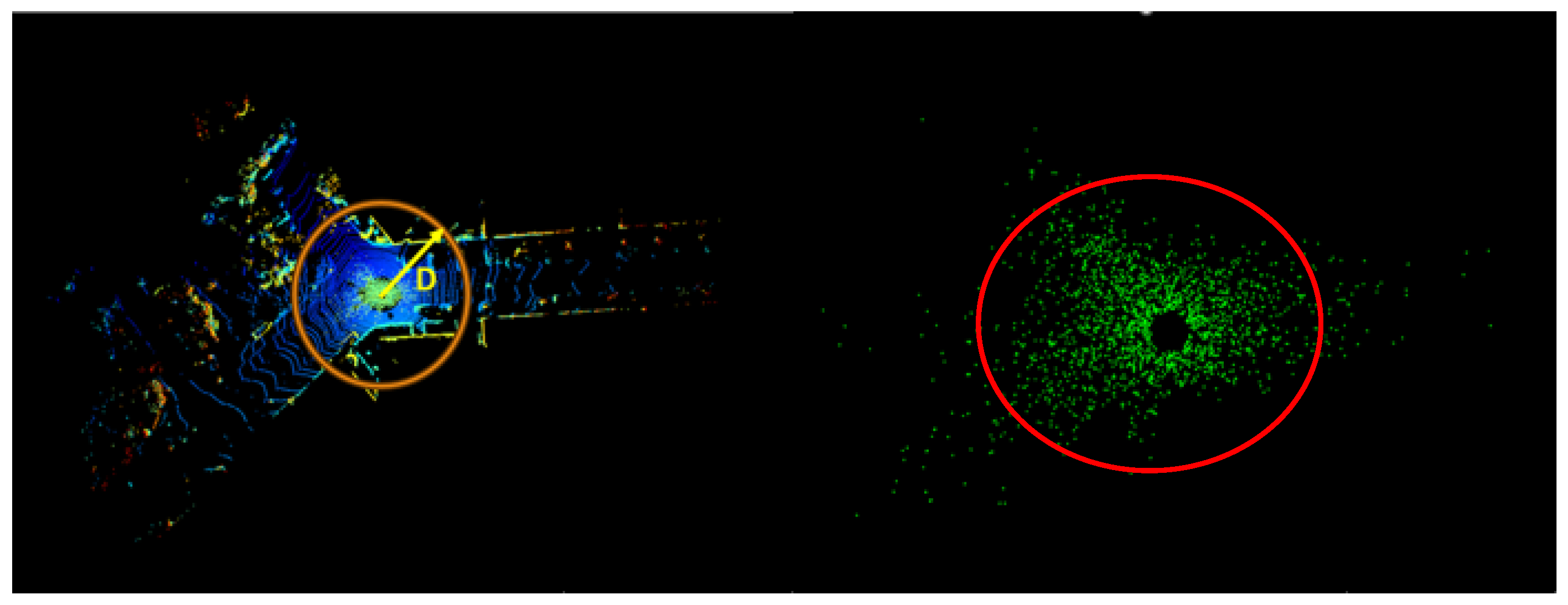
Compared to the complete point cloud, the circle includes all the noise points and some normal environment objects, as shown in Figure 3 and Figure 4. The noises within these two figures are nearly the same. This meets the training requirements for the point cloud denoising task, ensures a consistent input size, reduces training requirements, and maximizes the preservation of the noise points. Specific data on data reduction are shown in

Table 1. Specific values for the reduction in the number of point clouds.

	Raw Data	Processed Data
All points	200,659	128,000
Noise points	21,489	20,447

. This ensures that the neural network can fully learn the characteristics of the noise points during subsequent training. In subsequent training, the neural network learns the characteristics of the noise points to the greatest extent possible.

In this study, the data distribution of WADS is analyzed. We standardized the number of input points to the network at 128,000 points, a sufficiently large number of noise points to be retained while reducing the data size. In Table 1, with the number of points dropping by 36.2%, the number of noise points only dropped by 4.8%. This means that the characteristics of the noise points are effectively preserved.

3.2. The Proposed Network

The network proposed in this paper introduces an inception structure, a residual structure, and parallel computation. The inception structure enables the network to handle various inputs, while the residual structure ensures the transmission of parameters even in extreme cases [22]. Additionally, the network achieves a similar effect to the traditional step-by-step network structure by using a lightweight structure with repetitive loops, without significantly increasing the network parameters. Similar results can be achieved using a lightweight structure with repetitive loops instead of the traditional incremental network structure. This approach does not significantly increase the network parameter scale, while the parallel structure maximizes hardware utilization and extracts multiple features simultaneously.

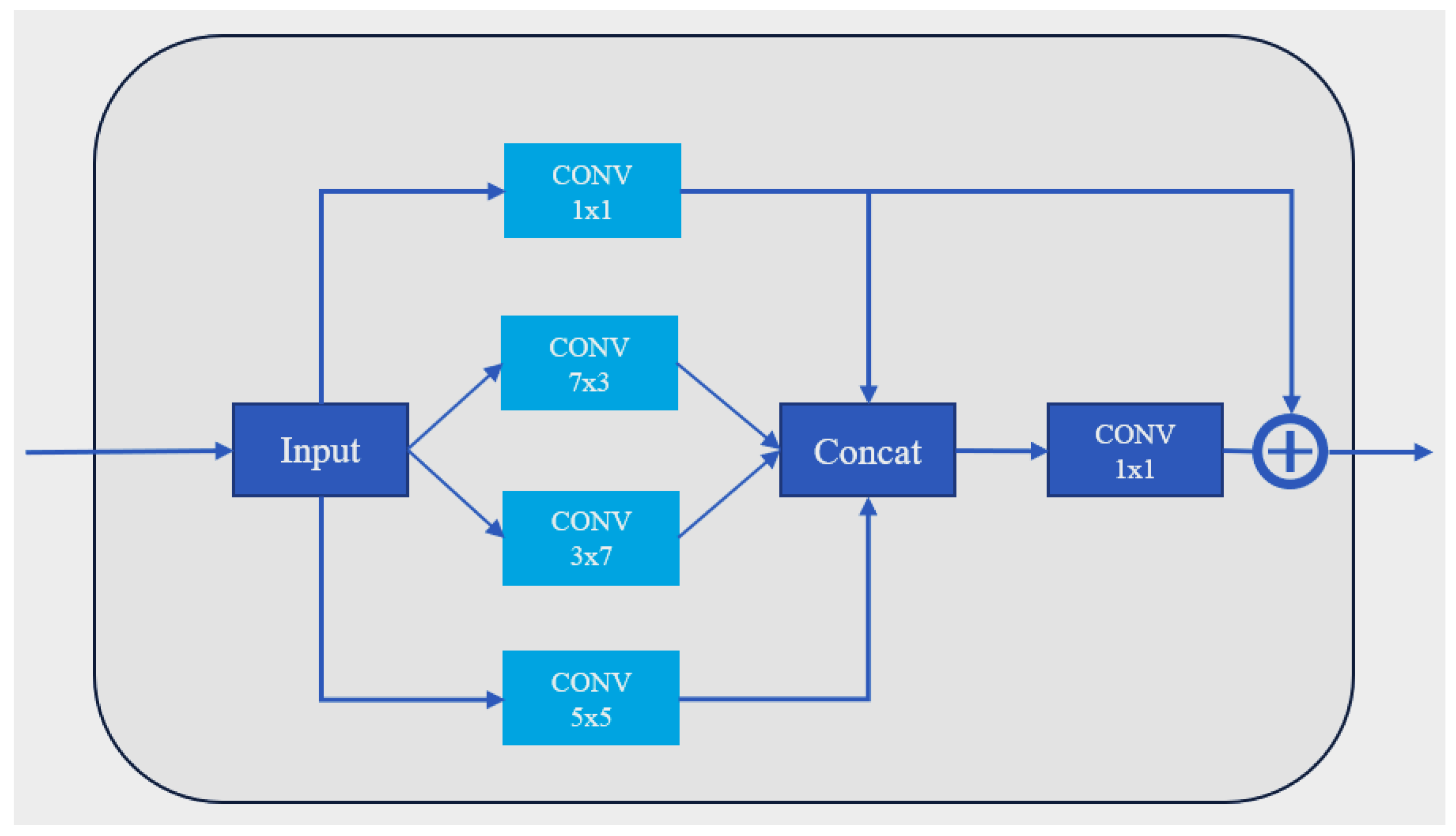
The base block in Figure 5 was designed to handle objects with different aspect ratios by containing filters of various sizes. Residual structures were added to construct the entire network based on this block. The block utilizes the inception layer proposed in GoogLeNet [21]. This block connects the outputs of multiple filters and a 1 × 1 filter to adjust the output dimension to a fixed size. The residual structure ensures that the parameters can be passed on in any case.

As the number of network layers increases, the traditional neural network structure will have more parameters, which can lead to a decrease in performance or even worse results. Additionally, a large number of parameters can significantly increase hardware requirements. Therefore, finding ways to achieve the desired effect without significantly increasing parameter size is necessary.

For this reason, residual and inception structures are in the blocks that make up the network. The residual structure introduces shortcuts so that a layer in the network can be directly connected to the previous layers via shortcuts. This direct gradient propagation path helps to alleviate the gradient vanishing problem and makes the gradient flow through the whole network more easily. Compared to traditional network structures, residual structures are less likely to reduce the gradient to too small a value during gradient propagation, thus better supporting deep network training.

The inception structure employs multi-scale convolutional kernels to effectively capture features at different scales, improving the model’s ability to recognize objects of varying sizes. Four types of convolution kernels were used: [1 × 1], [7 × 3], [5 × 5], and [3 × 7]. The [3 × 7] and [7 × 3] kernels have non-traditional lengths to accommodate inputs with varying dimensions, such as those with a larger difference between length and width. The [5 × 5] kernel is of a traditional size and is used for regular inputs.

Three parameters from the Lidar system are input into the network: distance, reflection intensity, and laser ID. The traditional method only utilizes distance and reflection intensity. However, after observing different datasets, we found that most of the noise points are distributed in a fixed area, as shown in Figure 6. The laser ID parameter can represent the relative height position of the point cloud. Through the input of this parameter into the network, it can learn additional features and focus on positions where noise points are more likely to appear, resulting in more effective noise identification.

The proposed network structure comprises two parallel neural networks. One is a traditional neural network constructed based on the block proposed above. The other is a lightweight, small-scale neural network structure that indirectly extracts more features through eight expansion and compression operations. This results in a larger receptive field with fewer parameters, achieving an effect similar to that of the classical neural network. The overall network structure is shown in Figure 7.

The neural network in its traditional form is not sufficiently equipped to identify noise points accurately. A parallel network structure capable of handling this situation is introduced to address this issue. To introduce additional networks without significantly increasing the network parameter size, a small network structure with alternating expansion and compression was used instead of the traditional network structure with continuous expansion and then continuous compression.

Conventional neural networks undergo successive expansion and compression phases. During the expansion phase, the parameter scale increases, leading to higher hardware requirements. Replacing the large-scale network structure with a repetitive smaller-scale network structure can achieve similar performance with fewer parameters. The alternating expansion and compression process increases the receptive field of the network, better capturing the long-range dependencies of the input data, while reducing computation and model complexity.

Theoretically, the more cycles, the better the network, but as the number of cycles increases, the depth of the network also increases. This action brings the risk of performance degradation and over-simulation and makes the network less effective [20]. Due to the hardware limitation, the computational performance is limited, so the number of cycles should be adjusted according to the actual hardware specification to strike a balance between performance and efficiency. After several experiments, six and eight cycles have been verified to achieve higher performance while still maintaining a relatively low computational cost, as shown in

Table 2. Training results for different numbers of structural cycles.

Structural Cycle Count	Training Cycle	Test Dataset Accuracy (%)	Network Runtime (s)
4	120	0.9728	0.026
5	120	0.9837	0.031
6	120	0.9850	0.034
7	120	0.9795	0.039
8	120	0.9853	0.043
10	120	0.9364	0.052

, which is a more ideal balance in the current experimental hardware environment; if the number of cycles is too small, it will affect the effect of noise identification, while too many cycles will be a bottleneck in the structure, which will slow down the speed of the entire network and cause poorer results due to the depth of the network. In the end, based on the evaluated parameters and the visualization of the filtering effect on the test dataset, eight cycles was chosen. However, six cycles is still an ideal choice; this action can be selected according to the actual situation.

The collaboration between the two networks enables the extraction of diverse features, enhances the model’s capacity to represent complex data, mitigates the risk of overfitting, and improves the network’s generalization ability. This results in more effective noise filtering of point clouds in complex scenarios. Additionally, the parallel structure maximizes hardware utilization.

In comparison to WeatherNet’s 1.6 M parameters, the proposed network has only 344 k parameters.

Table 3. GPU memory usage for different training batch sizes.

Training Batch Size	GPU Memory Usage (GB)
Batch Size	WeatherNet	RLFN
1	2.8	1.1
2	4.7	1.8
3	6.7	2.5
4	8.8	3.1
5	11	3.8
6	13.1	4.3
7	14.7	4.9
8	17.2	5.6

and Figure 8 display the hardware usage of various batch sizes during training. It is evident that the proposed network significantly reduces GPU memory usage. This enables the network to be trained and deployed on lower-specification hardware.

To address the contribution of individual components in the proposed Repetitive Lightweight Feature-preserving Network (RLFN) architecture, an ablation study was performed using WADS. This study systematically removed or altered specific elements of the network to observe the resulting effect on performance. The three components under examination were as follows: (1) Laser ID as an additional input—This feature encodes vertical spatial information, which aids in identifying noise distribution in adverse weather. (2) Inception modules—These capture multi-scale features, allowing the model to identify noise patterns across different spatial resolutions. (3) Dual-network structure—This includes the parallel architecture of a standard network branch and a lightweight expansion–compression branch to enhance feature diversity while minimizing computational load. (4) Analysis of the above combination—Excluding both laser ID and inception modules caused the most significant drop in performance, confirming that these components work synergistically to enhance model robustness.

4. Performance Analysis

Experiments were conducted on WADS to validate the proposed method’s effectiveness. The experimental results were compared with other methods on the same dataset. This chapter briefly presents information about the test dataset in its first part. In its second part, the experimental results of the proposed method are compared with the ROR, SOR, DROR, DSOR, and LIOR methods to evaluate the effectiveness of the proposed filtering method.

4.1. Experimental Dataset

This study utilizes the Winter Adverse Driving DataSet (WADS), which comprises environmental data collected during snowy weather. The dataset contains many snow-caused noise points and is labeled with various targets, including vehicles, buildings, vegetation, roads, snow, and eight other annotations. The dataset was collected by various sensors mounted on vehicles traveling on actual roads. The dataset covers various environments such as suburbs, cities, bridges, and highways from different regions and countries. It also includes a range of weather conditions, from light to heavy snowfall, making it suitable for training and validating deep learning algorithms.

WADS is designed to enhance autonomous driving in unfavorable weather conditions. Its extensive data collection provides researchers with valuable resources for training and validation, enabling them to make greater contributions to improving the robustness and reliability of automated driving vehicles.

For training purposes, sequences 11 to 26 (11, 12, 13, 14, 15, 16, 17, 18, 20, 22, 23, 24, 26) were used, which constitute 70% of the total dataset. Sequences 30 to 76 (30, 34, 35, 36, 76) comprise the test set, representing 25% of the total dataset. Sequence 28 is the validation set, comprising 5% of the total dataset.

4.2. Evaluation Metrics

There are five metrics used to evaluate a filter’s ability to cancel noise in adverse weather conditions: accuracy, precision, recall, F1 score, and inference time. The first four metrics are calculated using the following equations:

$$Accuracy={\displaystyle \frac{TP+TN}{TP+FP+TN+FN}}$$

$$Precision={\displaystyle \frac{TP}{TP+FP}}$$

$$Recall={\displaystyle \frac{TP}{TP+FN}}$$

$$F1score=2\ast {\displaystyle \frac{Precision\ast Recall}{Precision+Recall}}$$

The four basic parameters are TP (True Positive), FP (False Positive), TN (True Negative), and FN (False Negative). We set noises as the positive case and objects as the negative case; then, TP stands for correctly predicting noises, FP stands for incorrectly predicting noises, TN stands for correctly predicting objects, and FN stands for incorrectly predicting objects.

Accuracy is the simplest measure on the whole justification, but if the difference between the number of positive and negative cases is too big, it will decrease its validity. Precision embodies the model’s ability to distinguish the negative case samples; the higher precision is, the stronger the model’s ability to distinguish the negative case samples is. Recall embodies the model’s ability to recognize the positive case samples; the higher recall is, the stronger the model’s ability to recognize the positive case samples is. The F1 score is a comprehensive evaluation of the two; the higher the F1 score is, the more robust the model is.

4.3. Implementation Results

The comparative evaluation was performed using Python 3.11. The experiments were conducted on a laptop with an AMD Ryzen 9 5900HX CPU @ 3.30 GHz, an NVIDIA GeForce RTX 3080 Laptop GPU, and 64 GB of RAM.

The efficiency of the filters was evaluated by comparing different metrics with the SOR, ROR, DROR, DSOR, and LIOR filters, as well as WeatherNet.

Table 4. Effectiveness comparisons of different filters on WADS.

	Acc (%)	Pre (%)	Recall (%)	F1 (%)	Mean Inference Time (s)	Standard Deviation (Accuracy)	Confidence Interval (Accuracy)	Hardware
SOR	79.57	32.73	21.96	26.98	0.12	±2.34	[77.23, 81.91]	CPU
ROR	62.50	67.79	18.19	28.68	0.17	±1.89	[60.61, 64.39]
LIOR	90.35	66.17	55.56	60.04	0.66	±1.12	[89.23, 91.47]
DROR	96.17	71.91	91.89	80.68	18.19	±0.98	[95.19, 97.15]
DSOR	95.77	65.07	95.60	77.43	0.12	±1.03	[94.74, 96.80]
WeatherNet	92.93	90.80	91.21	91.78	0.046	±0.76	[92.17, 93.69]	GPU
RLFN	98.53	96.28	96.48	96.31	0.043	±0.45	[98.08, 98.98]

shows the efficiency comparisons of the different filters.

Performance evaluation utilizes several metrics, such as accuracy, precision, recall, and F1 score. It is evident that conventional noise filtering methods are ineffective in filtering out target points, despite their simple structure and faster processing time.

The term “inference time” refers to the time taken by the model to process a single batch of input data and generate the output predictions. This includes the time required for the forward pass through the neural network but does not include pre-processing and I/O time. To clarify, the inference time is computed as follows: (1) Forward pass time—This is the time taken for the neural network to process the input data and produce the output. (2) Exclusion of pre-processing and I/O time—The pre-processing steps (e.g., data normalization, feature extraction) and input/output operations (e.g., reading data from disk, writing results to disk) are not included in the inference time measurement.

Conversely, the LIOR filter significantly improves recall, and its intensity-based noise filter can effectively enhance noise filtering capability. However, the LIOR filter does not categorize point clouds with lower reflection intensity. The DROR and DSOR filters exhibit higher accuracy and recall rates, but their accuracy is still unsatisfactory. This lower accuracy results in the loss of valuable data in the point clouds, ultimately affecting target identification and driver safety.

The deep learning-based methods show obvious advantages, and their various metrics are satisfactory. The proposed method achieves even better performance metrics without significantly increasing the computation time by reducing the size of the neural network, and the hardware requirements are also reduced due to the reduced size of the neural network.

Since the traditional method relies only on the CPU, its speed is limited. On the other hand, deep learning methods can rely on GPUs for accelerated computation, which dramatically increases speed. Due to the scalable nature of GPUs, deep learning can easily improve computational efficiency by deploying more powerful GPUs or multiple GPUs.

In Table 4, the proposed method is improved in various aspects compared to other methods:

• Accuracy: WeatherNet (+5.60%), DSOR (+2.76%), DROR (+2.36%), and LIOR (+8.18%).
• Precision: WeatherNet (+5.48%), DSOR (+31.21%), DROR (+24.31%), and LIOR (+30.11%). This suggests that the proposed filtering method is effective in retaining important object points.
• Recall: WeatherNet (+5.27%), DSOR (+0.88%), DROR (+4.59%), and LIOR (+40.92%). This shows that the proposed filtering method effectively filters out the noise points.
• F1 score: WeatherNet (+4.53%), DROR (+18.88%), DROR (+15.45%), and LIOR (+36.27%). This shows that the proposed filtering method strikes a good balance between noise removal and physical retention.

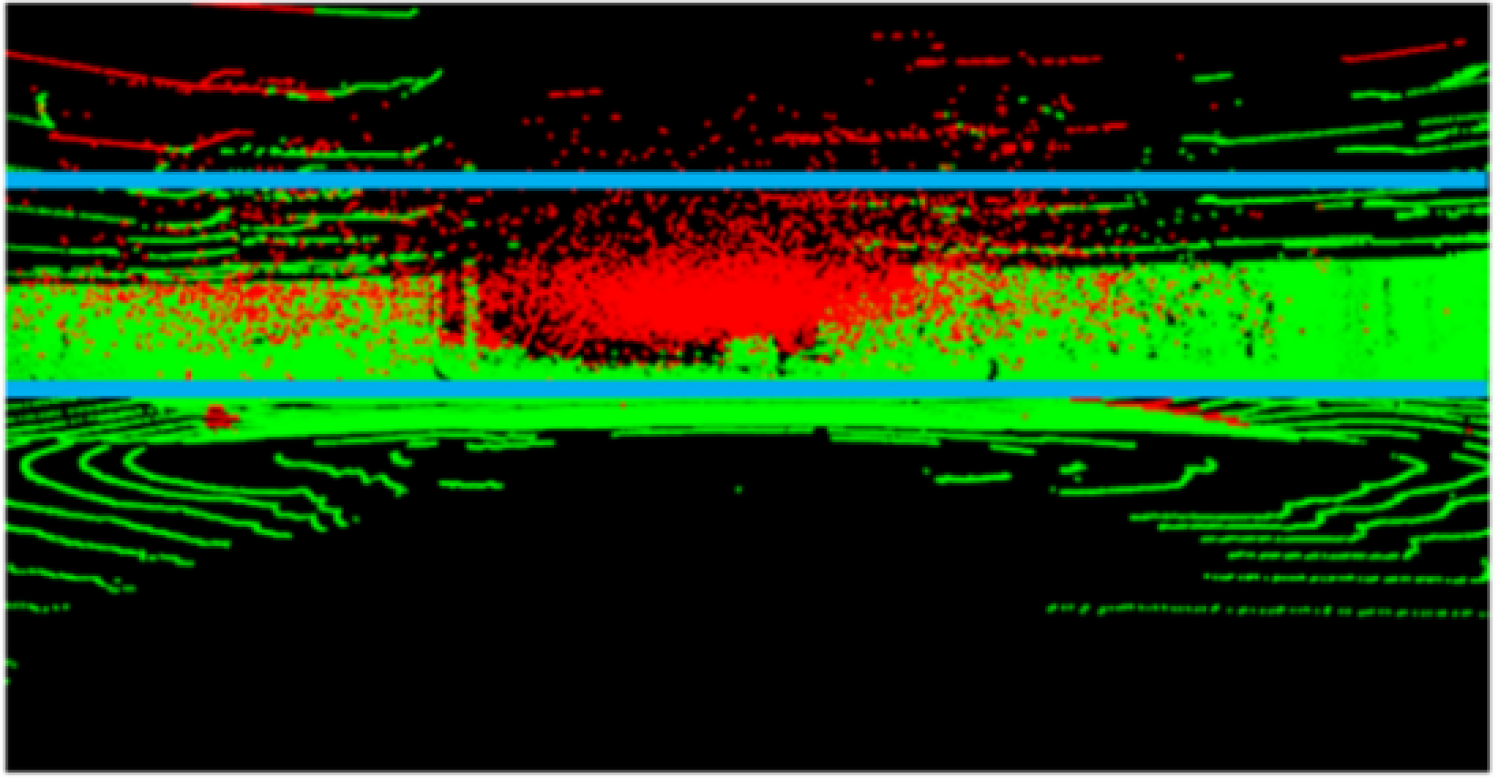
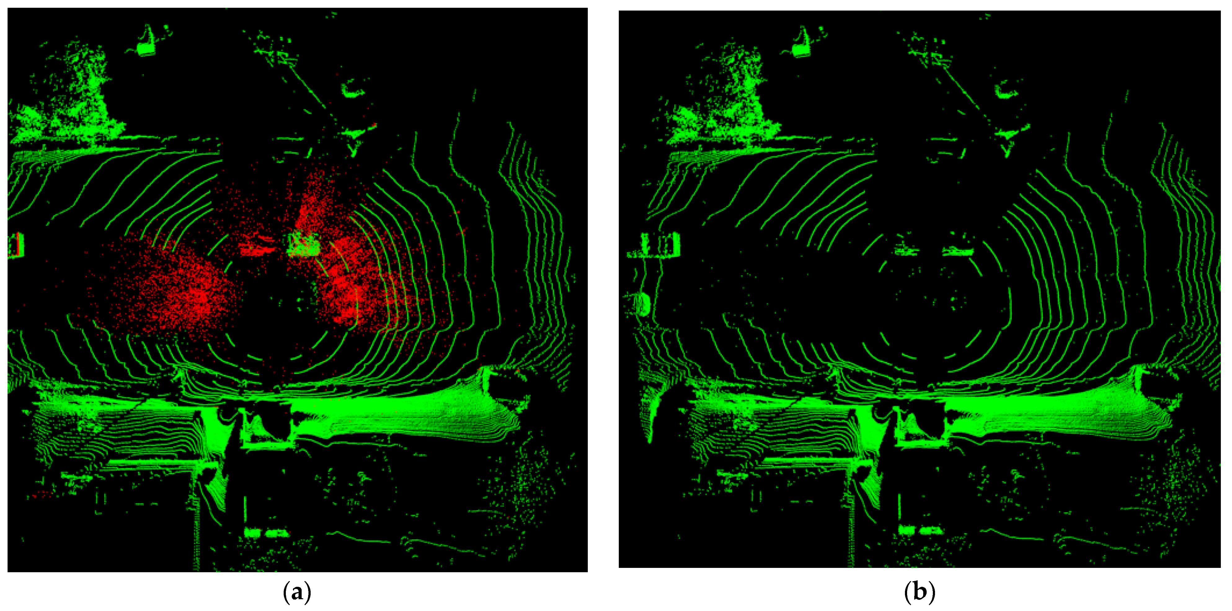
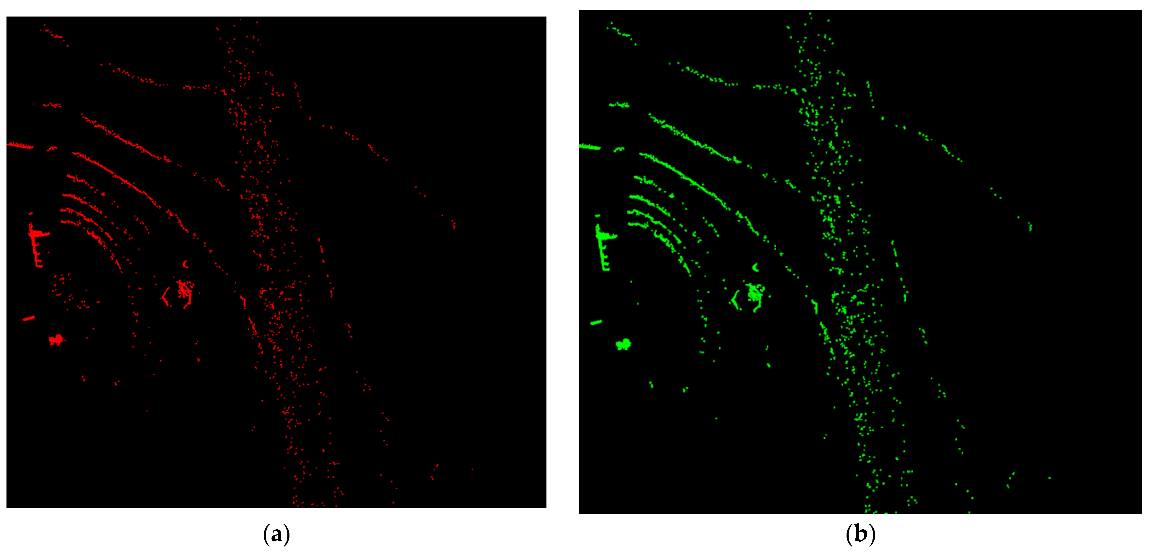
Figure 9 and Figure 10 demonstrate the filtering effect by the proposed method and WeatherNet, respectively. The figures show that the proposed method effectively removes most noise points while retaining most objects. In contrast, WeatherNet misses a significant amount of noise.

Table 5. WeatherNet’s noise removal and object retention results.

	Average Forecast Number	Average Total Number	Percentage (%)
Noise	11,365	13,130	86.56
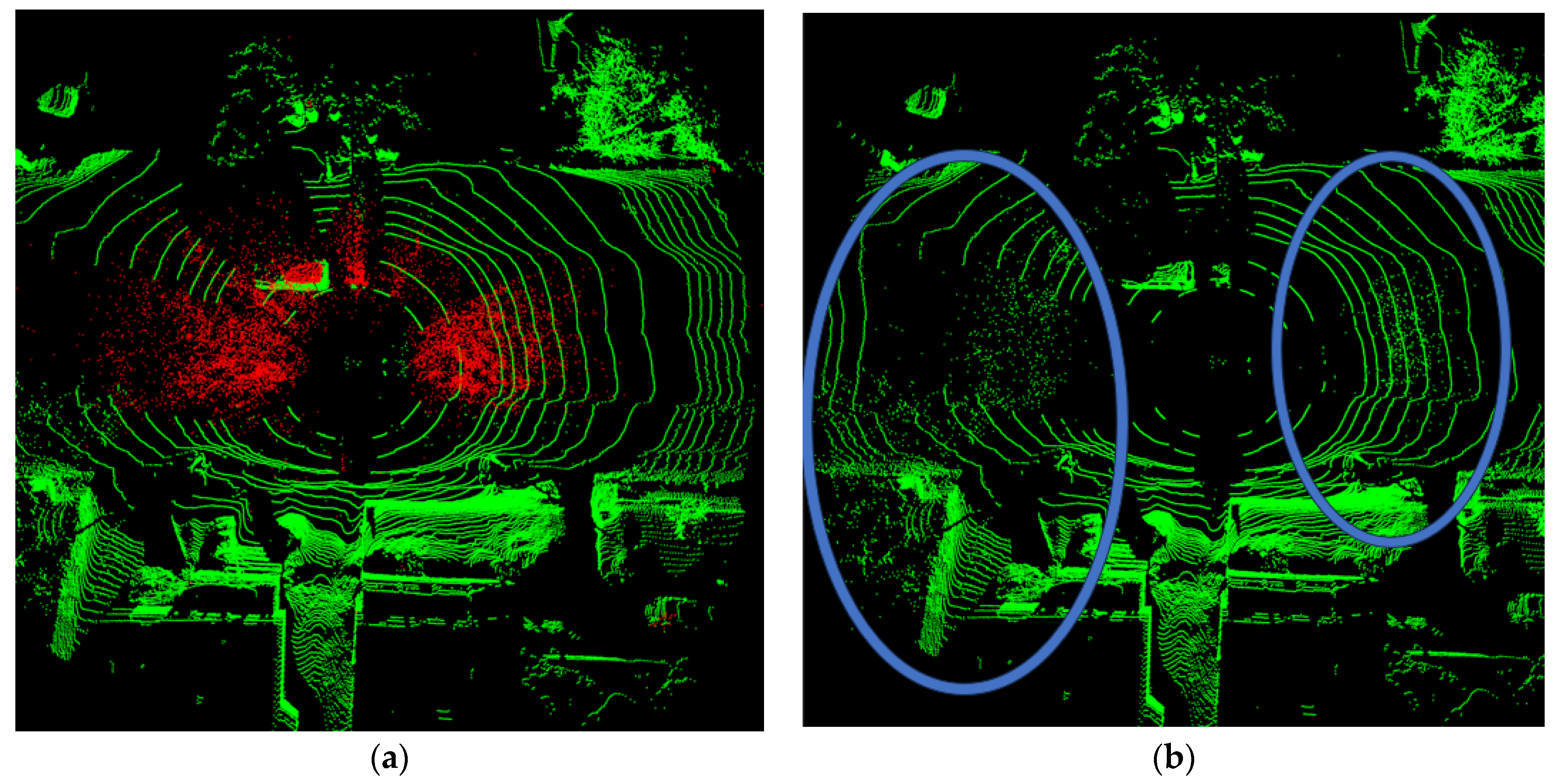
Object	112,883	114,870	98.27

and

Table 6. RLFN’s noise removal and object retention results.

	Average Forecast Number	Average Total Number	Percentage (%)
Noise (Removed)	12,330	13,130	93.91
Object (Preserved)	113,747	114,870	99.02

compare noise filtering and object retention between the two methods. It is evident that the proposed method retains object points effectively while removing more noise.

The proposed method retains 0.75% more object points while removing 7.53% more noise points than WeatherNet.

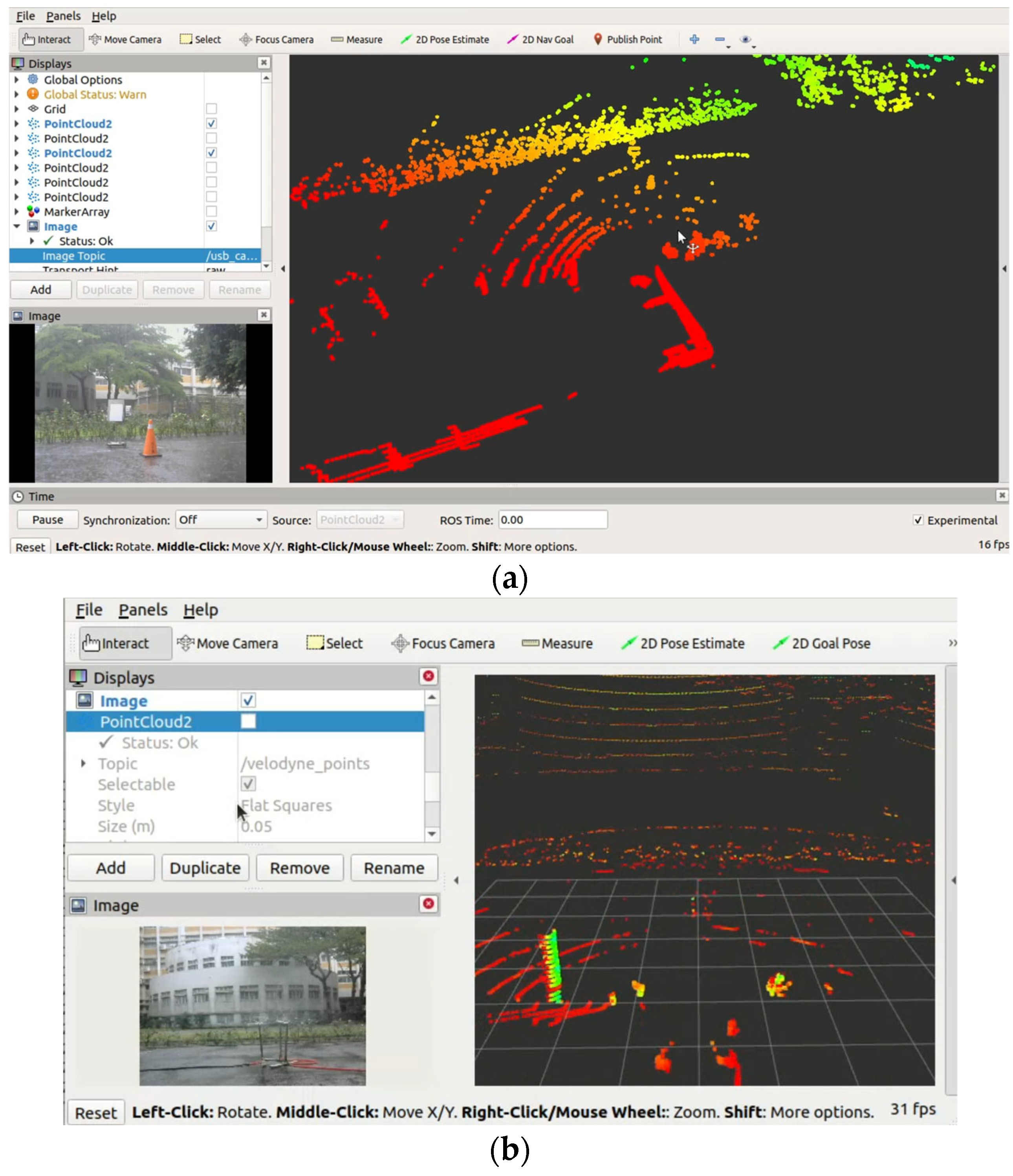
4.4. Real Environment Validation by a LiDAR System

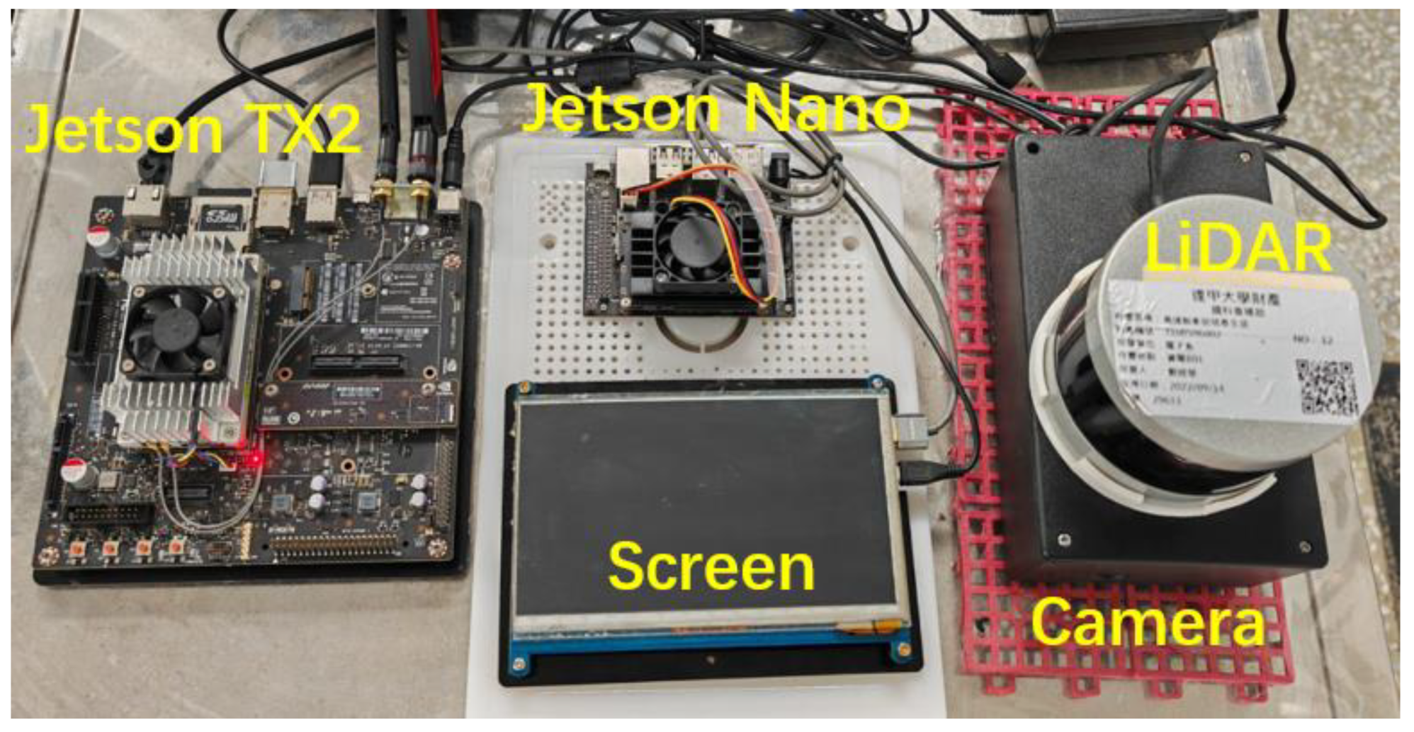
To verify the effectiveness of the proposed methodology in real-world environments, an actual LiDAR system was assembled. This hardware system mainly uses LiDAR data acquisition and camera image processing. An embedded platform from NVIDIA, Jetson Nano and Jetson TX2, is used to collect data from the sensor system. The signal processing system is based on the ROS2 platform under the Ubuntu environment, combining C++ and Python languages.

Figure 11 shows the architecture of the LiDAR hardware system, which comprises three main components: the Jetson Nano/Jetson TX2, LiDAR VLP-16, and a camera. The Jetson Nano/Jetson TX2 receives and processes data from LiDAR VLP-16 and the camera, generating output for further analysis and decision-making. The Jetson Nano/Jetson TX2’s graphics processor can be used by the system to process data in real time, allowing for the efficient integration of LiDAR and camera inputs. LiDAR is connected to the system through an Ethernet port, while the camera is connected through a USB interface. Both devices perform data acquisition simultaneously.

The LiDAR system consists of Jetson Nano/Jetson TX2, LiDAR VLP-16, and a camera, as shown in Figure 12, which combines the strengths of LiDAR and camera technologies to move through real-time contrasts of video and point clouds to achieve an accurate and comprehensive understanding of the environment.

The physical characteristics of the Velodyne VLP-16 LiDAR sensor used in our experiments include its 360° horizontal field of view, 30° vertical FOV, 10–20 Hz scanning frequency, 0.2° angular resolution, and 300,000 points/second acquisition rate.

The real justification in heavy rain and emulation situations are both used. We clarify that in our rain emulation, real water droplets were used via sprinklers, and no artificial noise generation model was applied. Thus, we did not simulate laser–rain interactions via a physical scattering model but rather validated the model using real rain-induced reflections. WADS similarly includes real snow-induced noise.

Combining Velodyne VLP-16 LiDAR with ROS2 provides a powerful and flexible platform for processing LiDAR data. The ROS2 node relationship is shown in Figure 13; two language nodes are used in ROS2, where the C++ node is responsible for accepting the raw data from VLP-16 and converting it into XYZ and other data for publishing, and then the Python node is used to receive and process the data. Then the processed point cloud data is published and then received by the visualization tool, Rviz2, for visualization.

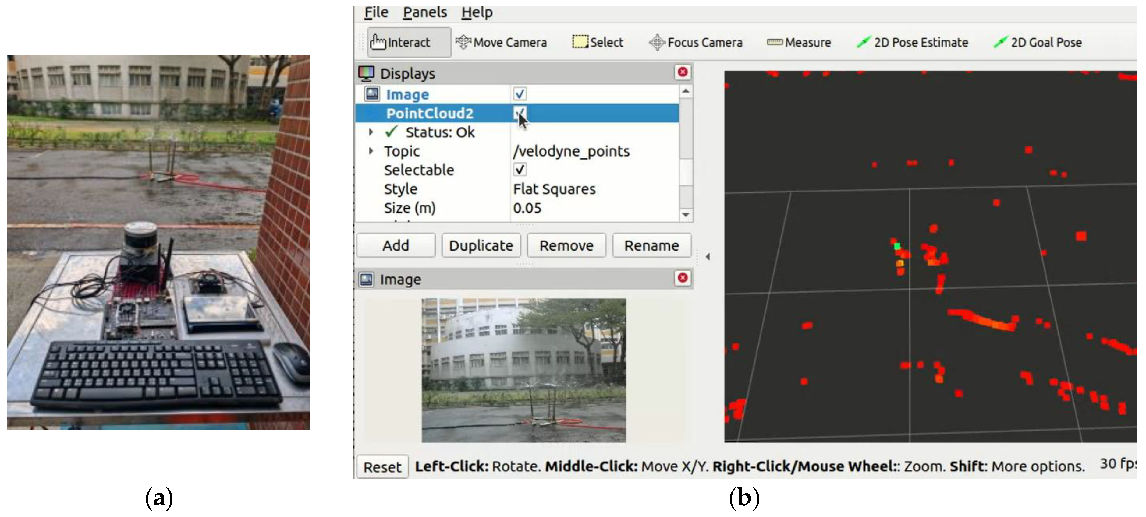
Due to the uncertainty of rainfall, this study uses an artificial method to simulate rainfall by placing three sprinklers in a centralized location to simulate a rainfall environment. Figure 14 shows the placement of the LiDAR system and water sprinklers. Figure 15 shows the data collected in rainy day scenarios. The validation demonstrated the effect of noise removal in a real environment. The results show that the proposed method satisfies filtration requirements. The proposed method has also been validated in a heavily rainy environment, proving that it can operate effectively in simple embedded systems, as shown in Figure 15 and Figure 16.

The processing speed is shown in Table 6 after testing in the LiDAR system—a PC with Intel CPU i5-12400F and NVIDIA GPU GTX 1650, running by Ubuntu 20.04.

There is a significant difference between the network speed and the overall speed. The time consumed at different process stages needs to be recorded to identify the bottleneck that leads to a larger sum of the two functionalities. The performance data is shown in

Table 7. LiDAR system running speed.

Hardware	Net FPS	Total FPS
Jetson Nano	10.9	5.4
Jetson TX2	11.2	7.3
PC	222.2	37

.

Table 8. Time consumption for different stages of data processing.

Hardware	Time (s)
	Input Format Conversion	Ground Removal	Point Reduction	Network Computing	Output Format Conversion	Total
Jetson Nano	0.0775	0.0015	0.0094	0.0921	0.0023	0.1828
Jetson TX2	0.0359	0.0011	0.0077	0.0889	0.0019	0.1355
PC	0.02	0.0003	0.0017	0.0045	0.0005	0.027

shows that converting to the cloud format takes longer time, partially due to the lower CPU performance. Jetson Nano and Jetson TX2 have CPU frequencies of only 1.5 GHz and 2.0 GHz, respectively, and their architecture is relatively simple, which slows down the overall speed.

4.5. Limitations

The proposed method provides a significant improvement for the regular operation of LiDAR in harsh weather environments, but it also has some limitations. Since deep learning algorithms rely heavily on a large number of labeled datasets for practical training, this poses a challenge in the current situation where labeled data is scarce and also affects the training results if the datasets themselves are not labeled accurately.

With the development of LiDAR, the number of laser beams is increasing, and LiDAR has developed from 16 to 64 or even 128 beams. Since our proposed method introduces the parameter of laser beam ID, the network needs to be retrained to adapt to different wires of LiDAR.

The proposed RLFN noise filtering technique has significant practical implications for enhancing the performance and safety of autonomous driving systems under adverse weather conditions. The following are some key aspects: (1) Enhanced safety in autonomous driving—By effectively filtering out noise caused by heavy rain, snow, and fog, the proposed method improves the reliability of LiDAR data. This leads to more accurate object detection and environment perception, reducing the risk of accidents and enhancing the overall safety of autonomous vehicles. (2) Real-time processing on embedded systems—The lightweight design of the proposed network allows it to run efficiently on simple embedded systems, such as the NVIDIA Jetson Nano and Jetson TX2. This capability is crucial for real-time applications in autonomous driving, where quick and accurate data processing is essential for making timely decisions. (3) Cost-effective deployment—The reduced hardware requirements of the proposed method enable its deployment on less expensive platforms. This makes advanced noise filtering technology accessible to a wider range of applications, including low-cost autonomous vehicles and other robotics systems. (4) Versatility across different environments—The adaptive pre-processing and robust network structures ensure that the method can handle various types of noise and adverse weather conditions. This versatility makes it suitable for deployment in diverse environments, from urban areas with dense traffic to rural regions with open spaces. (5) Integration with multi-sensor systems—The proposed method can be integrated with other sensor modalities, such as cameras and radar, to create a comprehensive perception system. This multi-sensor approach enhances the overall situational awareness of autonomous vehicles, leading to better decision-making and improved safety. (6) Scalability and future-proofing—The scalable nature of the proposed method allows it to be adapted to future advancements in LiDAR technology, such as higher-resolution sensors and increased laser beam counts. This ensures that the method remains relevant and effective as technology evolves. (7) Potential applications beyond autonomous driving—While the primary focus is on autonomous driving, the proposed noise filtering technique can also be applied to other fields that rely on LiDAR data. These include robotics, environmental monitoring, and infrastructure inspection, where accurate and reliable data is crucial for effective operation for future applications.

The proposed approach is currently entering an emerging niche: the robustness of LiDAR systems under adverse weather conditions. The proposed method demonstrates its potential to significantly enhance the performance and safety of autonomous systems in real-world scenarios. Future work is needed to validate the robustness and generalization of our model; we plan to conduct additional experiments on diverse datasets that encompass various adverse weather conditions and environments. These datasets will include the following: (1) foggy weather—evaluating the model’s performance in foggy conditions to assess its ability to filter out noise caused by low visibility; (2) snowy weather—testing the model on datasets with heavy snowfall to ensure it can effectively remove noise from snow particles; (3) urban and rural environments—assessing the model’s robustness in different environments, such as urban areas with dense traffic and rural areas with open spaces. By demonstrating the model’s effectiveness across diverse scenarios, we aim to establish its reliability and applicability in real-world autonomous driving systems. This will contribute to the development of safer and more reliable autonomous vehicles capable of operating under various adverse weather conditions.

While U-Net, GANs, and transformer-based architectures are valuable in many domains, they often require significant computational resources and are not tailored to operate on raw LiDAR point clouds in real time. In contrast, RLFN is designed to operate efficiently in sparse, high-dimensional data environments and demonstrates strong trade-offs between accuracy, speed, and hardware feasibility, making it particularly suitable for embedded deployment in autonomous driving systems.

5. Conclusions

The proposed deep learning network’s noise filtering technology can effectively reduce noise interference from adverse weather conditions in LiDAR applications. The rain removal technique was validated on WADS, demonstrating its effectiveness in reducing the number of rain (noise) points during data collection. The accuracy and F1 score of the proposed method were 96.28% and 96.31%, respectively, indicating that the method effectively removes noise points while retaining object points in a balanced manner. Through the evaluation of a LiDAR system, the proposed technique can be run in simple embedded systems and deployed in heavy rain experiments by real-time processing.

Furthermore, the hardware requirements are significantly decreased due to the relatively small number of parameters in the network, and the data size is reduced by the proposed pre-processing method. This allows for training and deployment on less powerful embedded systems. Additionally, the effective utilization of GPUs for computation results in better performance compared to traditional methods. This technique enhances LiDAR’s ability to sense the vehicle’s surroundings accurately and reliably, thereby improving the safety and reliability of the autonomous driving system under heavy rain.