Next Article in Journal
Switchable Filter with Four Operating Modes Implemented on a 50-Ohm Microstrip Line
Previous Article in Journal
Direct Interface Circuits for Resistive, Capacitive, and Inductive Sensors: A Review
Previous Article in Special Issue
A Self-Supervised Point Cloud Completion Method for Digital Twin Smart Factory Scenario Construction
 
 
Due to scheduled maintenance work on our database systems, there may be short service disruptions on this website between 10:00 and 11:00 CEST on June 14th.
Article

DataMatrix Code Recognition Method Based on Coarse Positioning of Images

Department of Electronic Science, Fujian Provincial Key Laboratory of Plasma and Magnetic Resonance Research, School of Electronic Science and Engineering, Xiamen University, Xiamen 361005, China
*
Authors to whom correspondence should be addressed.
Electronics 2025, 14(12), 2395; https://doi.org/10.3390/electronics14122395
Submission received: 21 February 2025 / Revised: 4 April 2025 / Accepted: 6 April 2025 / Published: 12 June 2025

Abstract

:
A DataMatrix (DM) code is an automatic identification barcode based on a combination of coding and image processing. Traditional DM code sampling methods are mostly based on simple segmentation and sampling of a DM code. However, the obtained DM code images often have problems such as wear, corrosion, geometric distortion, and strong background interference in practical scenarios. To improve decoding ability in complex environments, a DM code recognition method based on coarse positioning of images is proposed. The two-dimensional barcode is first converted into a one-dimensional waveform using a projection algorithm. Then, the spacing between segmentation lines is predicted and corrected using an exponential weighted moving average model for adaptive grid division. Finally, the local outlier factor algorithm and local weighted linear regression algorithm are applied to predict and binarize the gray level values, converting the DM code image into a data matrix. The experimental results show that this method effectively handles problems like blurring, wear, corrosion, distortion, and background interference. Compared to popular DM decoding libraries like libdmtx and zxing, it demonstrates better resolution, noise resistance, and distortion tolerance.

1. Introduction

A DM code is an automatic identification barcode based on the principles of combination coding and computer image processing technology, invented by the American International Data Matrix company in 1989 [1]. A DM code is divided into two types: ECC000-140 and ECC200. ECC000-140 uses various levels of convolutional error correction methods, while ECC200 uses the Reed–Solomon algorithm for error correction. This article focuses on the ECC200 type of DM code. A complete DM code consists of the following parts [2], as shown in Figure 1.
  • Data regions: A matrix arranged according to certain rules, containing encoded data information. Dark and light modules represent binary “1” and “0”, respectively, as shown in Figure 1b.
  • Finder pattern: The finder pattern is a perimeter to the data region and is one module wide. The two adjacent sides illustrated in Figure 1c form the L boundary, and the two opposite sides illustrated in Figure 1d are made up of alternating dark and light modules. The finder pattern is used to locate and define the size of data modules, helping to determine the physical size and distortion of the barcode.
  • Quiet zone: This is one data module wide, mainly used to separate the two-dimensional barcode from background information, as shown in Figure 1e.
  • Alignment pattern: When the barcode symbol consists of multiple data regions, the data regions need to be divided by alignment patterns, as depicted in Figure 1f.
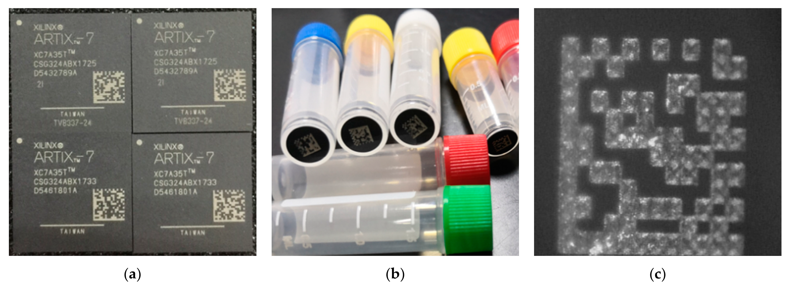
DM code has the smallest printable size among current two-dimensional barcodes [3] and can store 30 digits in an area of 25 mm. It also has excellent error correction capabilities, with a maximum of only 20% of barcode information required for accurate identification [4]. Due to its distinctive recognition capabilities [5], strong anti-pollution ability, small size, and large coding capacity, a DM code is widely used in Direct Part Marking [6,7,8,9], as shown in Figure 2. This type of barcode generation usually uses printing, photolithography, etching, impact, stamping, and other methods to encode on the surface of products or parts. However, due to the variety of barcode generation methods, the shape of code blocks may not be standard squares and the spacing between code blocks may be inconsistent. How to accurately locate and sample barcodes is an urgent research topic.
The decoding steps of a DM code can be roughly divided into DM code image input, DM code image preprocessing, DM code detection and positioning, DM code image correction and recognition, and DM code error correction and decoding. DM code image preprocessing mainly includes image graying, image enhancement, image denoising, and image binarization. Among them, the methods of image denoising mainly include Gaussian filtering [10], median filtering [11], and mean filtering [12]; the methods of image binarization mainly include OTSU [13], local threshold [14], maximum entropy threshold [15], Bernsen [16], and histogram bimodal [17]. DM code detection and positioning mainly include coarse positioning of a DM code and precise positioning of a DM code. Among them, the methods of coarse positioning of DM codes mainly include the method of locating candidate regions of DM codes based on corner point distribution [18], the positioning method based on mathematical morphology [19], the connected component labeling method [20,21], and the edge detection method based on the Sobel operator [22]. The methods for precise positioning of DM codes mainly include edge detection methods based on the Hough transform [23,24,25], edge detection methods based on the convex hull algorithm [26], and positioning methods based on the Radon transform [27]. The methods for correcting DM code images mainly include using a six-parameter affine transformation formula [28] and an eight-parameter affine transformation formula [29,30]. DM code image sampling methods mainly include binarization based on the proportion of black or white pixels in all pixels in each grid, binarization by counting the proportion of black and white pixels on the central cross-shaped symbol in the sampling grid, and binarization based on scanning the central pixel in the sampling grid. After converting the recognized DM code image into a data matrix, a codeword stream can be obtained. After error correction using the Reed–Solomon algorithm, information can be decoded.
At present, research on DM code decoding mainly focuses on DM code detection and positioning, and there is relatively little research on DM code image sampling, which is basically based on simple segmentation and sampling based on the coding of DM codes. However, due to the limitations of practical application scenarios, the obtained DM code images often have problems such as wear, corrosion, geometric distortion, and strong background interference. Traditional DM code image sampling methods can no longer meet the requirements. In fact, even state-of-the-art deep learning-based recognition systems have been shown to be vulnerable to slight input perturbations, where minimal noise added to the input can lead to completely incorrect recognition results, as demonstrated in recent studies on adversarial examples in AI systems [31]. To improve the decoding ability of DM codes in complex environments, this paper attempts to start from the aspect of DM code image sampling. By dividing adaptive sampling grids and binarizing based on grid grayscale change trends, the sampling grid division and data extraction steps in the DM code image recognition process are optimized to resist problems such as wear, corrosion, geometric distortion, and strong background interference in practical application scenarios and improve the decoding ability of DM codes.
The main contributions of this paper are as follows.
  • Based on the projection algorithm and the exponential weighted moving average model, an adaptive sampling grid division method is proposed to overcome the problem that the sampling grid cannot be divided when the finder pattern encounters pollution or is missing.
  • By combining the local outlier factor (LOF) algorithm and the local weighted linear regression algorithm, a binarization method based on grid grayscale change trends is proposed. It optimizes problems such as blurry DM code images, wear, corrosion, geometric distortion, and strong background interference in practical application scenarios. It reduces the quality requirements for DM code images and improves decoding capabilities in complex environments.
The rest of this paper is organized as follows. Section 2 briefly introduces the related work conducted in the field of DM code decoding. Section 3 introduces the adaptive sampling grid division method after the coarse positioning of DM code images. Section 4 introduces a binarization method based on grayscale change trends after sampling grid division. Section 5 describes the experiments and result analysis. Section 6 summarizes the paper.

2. Related Work

In the field of DM code image recognition, many researchers have proposed their own methods. These methods generally focus on the preprocessing, detection and positioning, and correction and recognition of DM code images. Many methods improve and optimize the algorithms for detecting, positioning, and correcting DM codes.
Ladislav Karrach et al. proposed an efficient algorithm for locating DM codes in images [7]. By using an improved local threshold segmentation technique and a connected component labeling method [32], image regions that may contain data matrix codes are identified; by analyzing the differences in adjacent projections around the finder pattern, the boundaries of the DM code are determined, thereby achieving the location of the DM code in the image.
Licheng Liao et al. proposed a novel laser-marked DM symbol reading method based on deep learning [33]. By training a convolutional neural network (CNN) model to learn the colors of two adjacent modules and label them depending on whether they have the same color or not, an edge image is generated based on the Kuhn–Munkres (KM) algorithm using the label matrix of DM code images. Finally, DM code images are reconstructed and decoded.
Tao Gao et al. proposed a DM code recognition technology based on corner detection and cluster analysis [20]. Firstly, noise and complex background interference are eliminated through image preprocessing; then, the initial positioning of two-dimensional barcode images is obtained through a method based on morphology. Finally, precise positioning is achieved based on corner detection and cluster analysis.
Dong Li et al. proposed an improved precise positioning method for DM codes [18], including four parts: fast positioning and priority sorting of DM code candidate regions based on corner point distribution, extraction of outer contours of DM code candidates, initial determination of the L side by using the improved Hough transform, and precise positioning of the L side by using iterative weighted least squares line fitting. Among them, the traditional Hough transform method needs to traverse every edge point in the image domain, and its computational efficiency is low; by improving the Hough transform based on trigonometric relationships and the characteristics of lines in polar coordinates, computational efficiency can be improved without reducing statistical points.
Wei Wang et al. aimed to combat the difficulty of locating DM codes under pollution and multiple perspectives, and proposed a precise positioning method for DM codes under pollution and multiple perspectives [34]. This method establishes a distribution model of internal edges of DM codes in the Hough domain under multiple perspectives and extracts features. The boundary combination corresponding to the maximum feature value is used as the final positioning result. The experiments show that this method has higher robustness for precise positioning of DM codes with scratches, wear, corrosion, geometric distortion, and other problems.
Wenting Cai et al. applied the concept of the convex hull in computational geometry to barcode positioning and proposed a DM code positioning method based on the convex hull algorithm [35]. The convex hull algorithm overcomes the disadvantage of traditional line detection algorithms based on the Hough transform which require a large amount of storage space due to global detection. The experimental results show that this algorithm can effectively locate distorted or tilted DM code areas.
Donghong Hu et al. extracted detection patterns according to the characteristics of detection boundaries in the Randon transform domain of two-dimensional barcode images [36] and verified through experiments that they can locate DM codes when the minimum module width of DM code images is only 2.7 pixels.
Xiao Lu et al. aimed to overcome problems such as noise and overexposure that often accompany industrial two-dimensional code recognition; they proposed an image enhancement algorithm based on gamma transform of top–bottom hat transforms to effectively reduce the impact of lighting. According to the characteristics of DM codes, they proposed a fast positioning algorithm for DM codes based on Shi–Tomasi corner point density by cleverly using internal block corner point information to achieve fast positioning [37].
It is not difficult to see from the above research work on DM codes that researchers mainly focus on image preprocessing and detection and positioning of DM codes. For positioned DM codes, researchers generally divide sampling grids based on finder patterns and take central pixels from sampling grids to convert recognized DM code images into data matrices. This paper improves the recognition method for positioned DM codes with the aim of recognizing low-quality DM code images and improving the decoding ability of DM codes in different environments.

3. Method of Adaptive Sampling Grid Partitioning

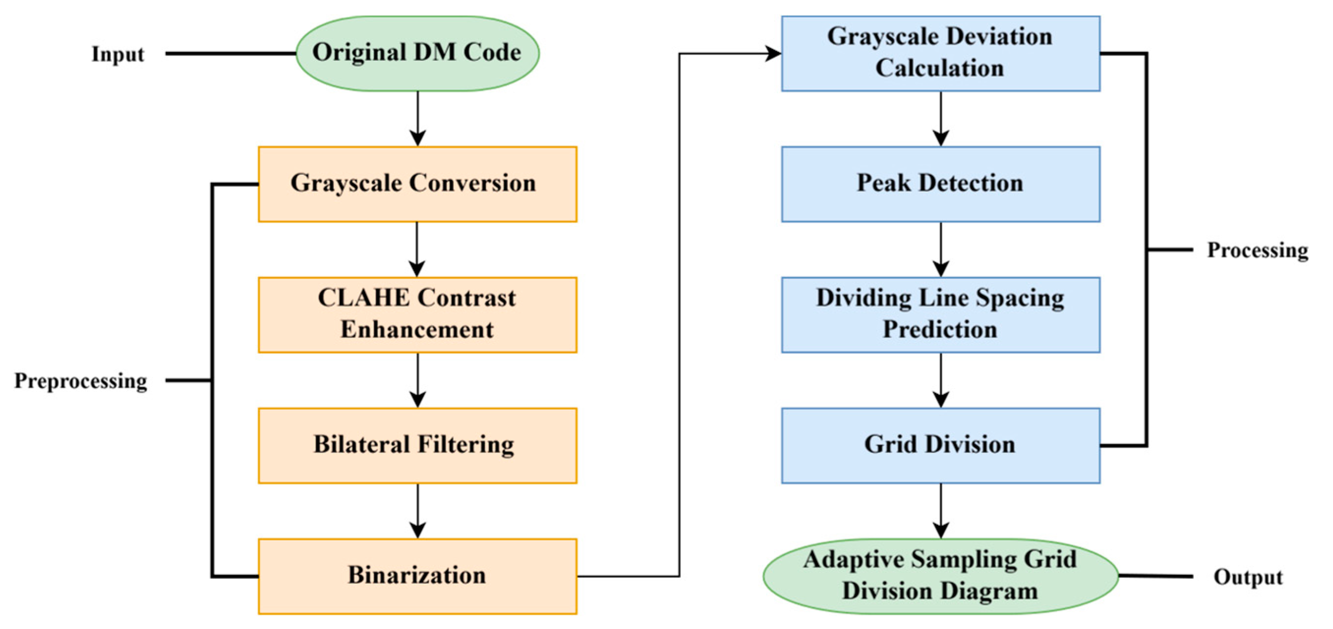
The division of the sampling grid is usually based on the finder pattern of DM codes [2], but when the finder pattern encounters pollution or is missing, it is no longer possible to divide the sampling grid by using this method. This section proposes an adaptive sampling grid division method, and the overall workflow is shown in Figure 3. By calculating the gray deviation value of the DM code image in one direction and accumulating it in the vertical direction, the two-dimensional barcode is converted into a one-dimensional waveform for analysis to obtain the sampling grid. The experimental results show that this algorithm can effectively divide the sampling grid of DM code images with problems such as wear, corrosion, geometric distortion, and strong background interference.

3.1. DM Code Image Preprocessing

After obtaining the coarsely positioned DM code image, the image is scaled to a pixel space of 256 × 256 by bilinear interpolation to ensure that the algorithm has similar performance on all images and can be better compared and analyzed.
Since this algorithm needs to calculate the gray value deviation between each pixel of the DM code image and its adjacent pixels and accumulate the gray value deviation, it has a certain sensitivity to image noise; but since this algorithm judges the overall waveform, it has good anti-blur performance. Therefore, filtering and binarization can be performed on the DM code image before dividing the adaptive sampling grid.
Bilateral filtering [38] is a nonlinear filtering method that can reduce noise while maintaining clear edges by combining information from the spatial domain and gray value domain. The OTSU13 method is based on the analysis of the image grayscale histogram and finds an optimal threshold to divide the image into two parts: background and foreground. This algorithm uses bilateral filtering and the OTSU method to carry out filtering and binarization operations on DM code images.

3.2. Waveform Extraction

The preprocessed image is converted into a gray value matrix, denoted as GreyMatrix, as shown in Equation (1):
G r e y M a t r i x = a 11 a 12 a 1 n a 21 a 22 a 2 n a n 1 a n 2 a n n 256 × 256 ,
where a i j represents the gray value of pixel p i , j , where i represents the row and j represents the column. Then, the cumulative gray deviation value of p i , j in the horizontal direction is shown in Equation (2):
f j = n = 1 256 a n j + 1 a n j ,     1 j 255 n = 1 256 a n j ,     j = 256 .
The cumulative gray deviation value of p i , j in the vertical direction is shown in Equation (3):
f i = n = 1 256 a i + 1 n a i n ,     1 i 255 n = 1 256 a i n ,     i = 256 .
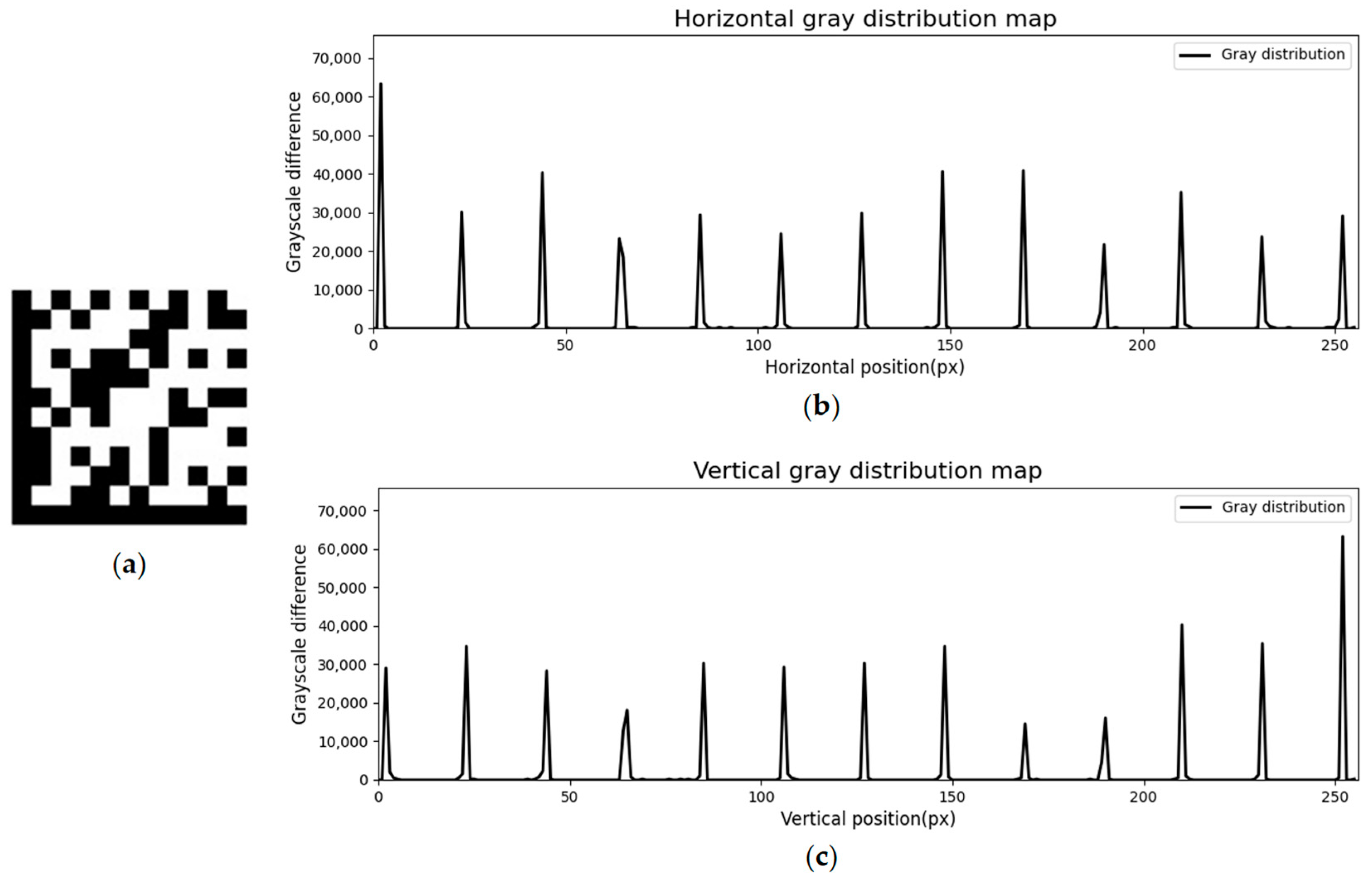
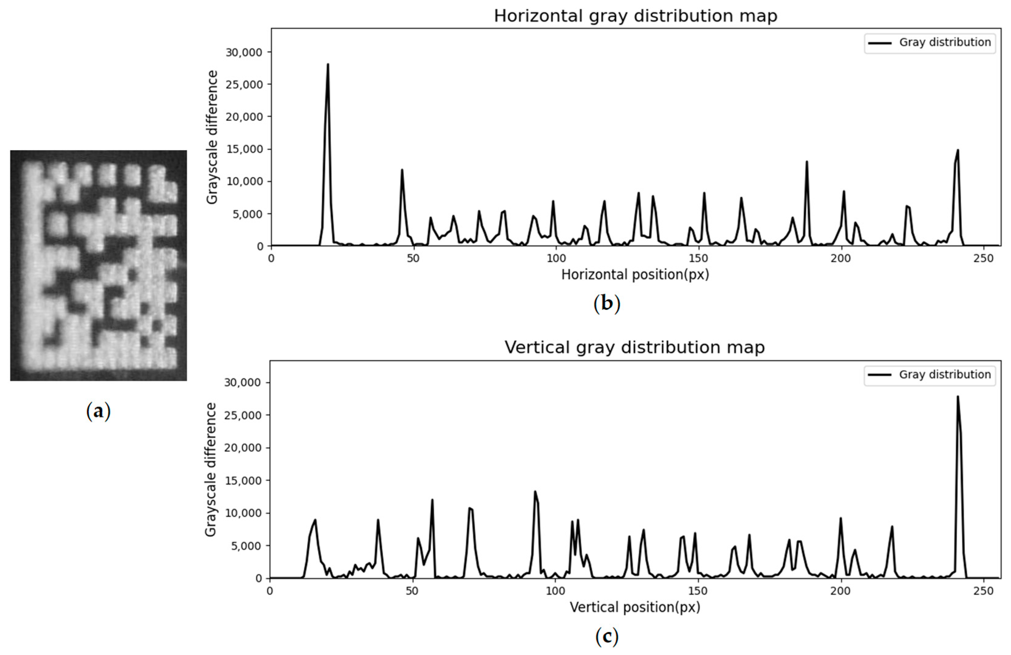
Figure 4b,c display the distribution of gray deviation values in the horizontal and vertical directions of Figure 4a, respectively. The two-dimensional barcode is transformed into a one-dimensional waveform for analysis.

3.3. Peak Detection

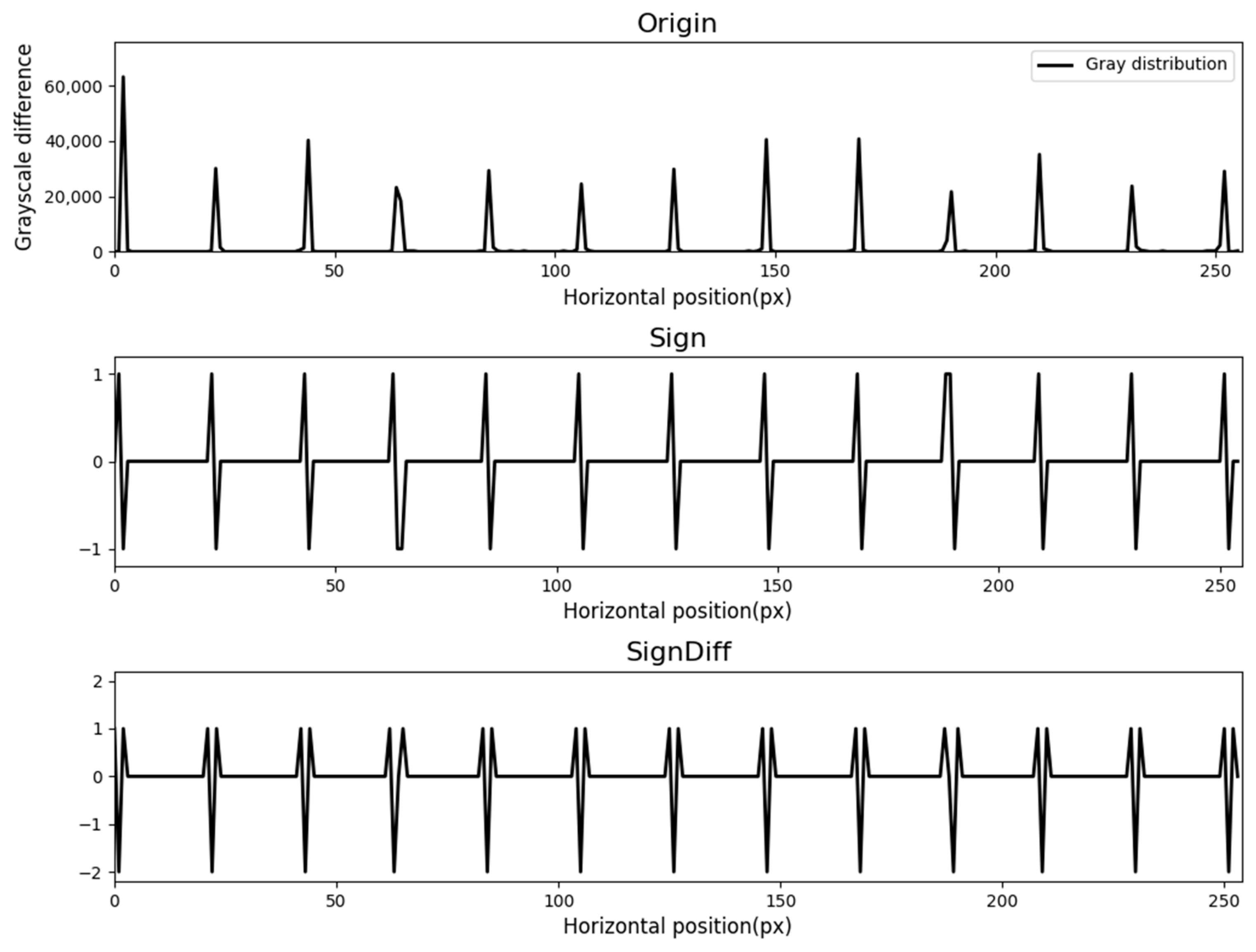
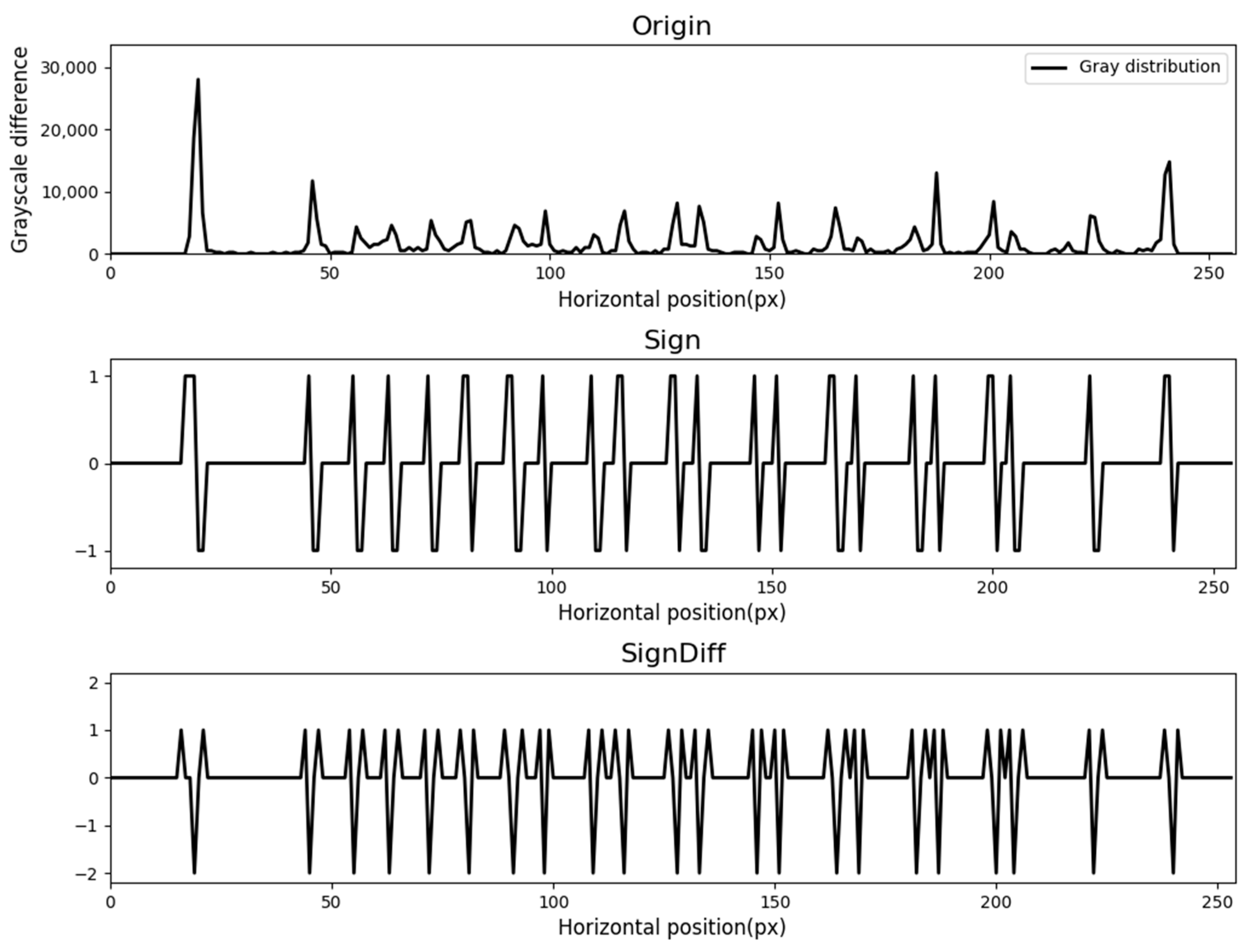
From the gray deviation value distribution map in Figure 4, it can be seen that at the junction of black and white grids, there is a peak value of gray deviation. Therefore, as long as the position of the peak is detected, the position of the dividing line can be found. It is necessary to calculate the first-order difference of the waveform to obtain the gradient direction map of the waveform. Among them, 1, 0, and −1, respectively, represent the rising, maintaining, and falling trends of the waveform. Then, one must take the difference in the gradient direction. When the results are 1 and 2, there are corresponding valleys; when the result is 0, the corresponding state remains the same; when the result is −2, there is a peak with a single extreme value; when the result is −1, there is a trapezoidal peak [39]. Figure 5 is a peak detection process diagram in the horizontal direction based on Figure 4b.
However, in real application scenarios, DM code images often have problems such as wear, corrosion, geometric distortion, and strong background interference. Figure 6a is a DM image obtained in an actual scene. There is a lot of interference in both horizontal and vertical directions, as shown in Figure 6b,c. Figure 7 is a peak detection process diagram in the horizontal direction based on Figure 6b. It can be seen that in actual application scenarios, it is necessary to screen the detected peaks to accurately find the peaks representing the position of the dividing line.

3.4. Dividing Line Recognition

Since there are peaks caused by wear, corrosion, geometric distortion, and background noise among the detected peaks, it is necessary to screen out the peaks representing the position of the dividing line from the detected peaks. This paper proposes a dividing line recognition method based on predicting the dividing line spacing. The dividing line spacing is predicted based on the detected adjacent peak spacing; the detected peaks are grouped based on the predicted dividing line spacing, and the position of the strongest peak in the group is defined as the dividing line position.
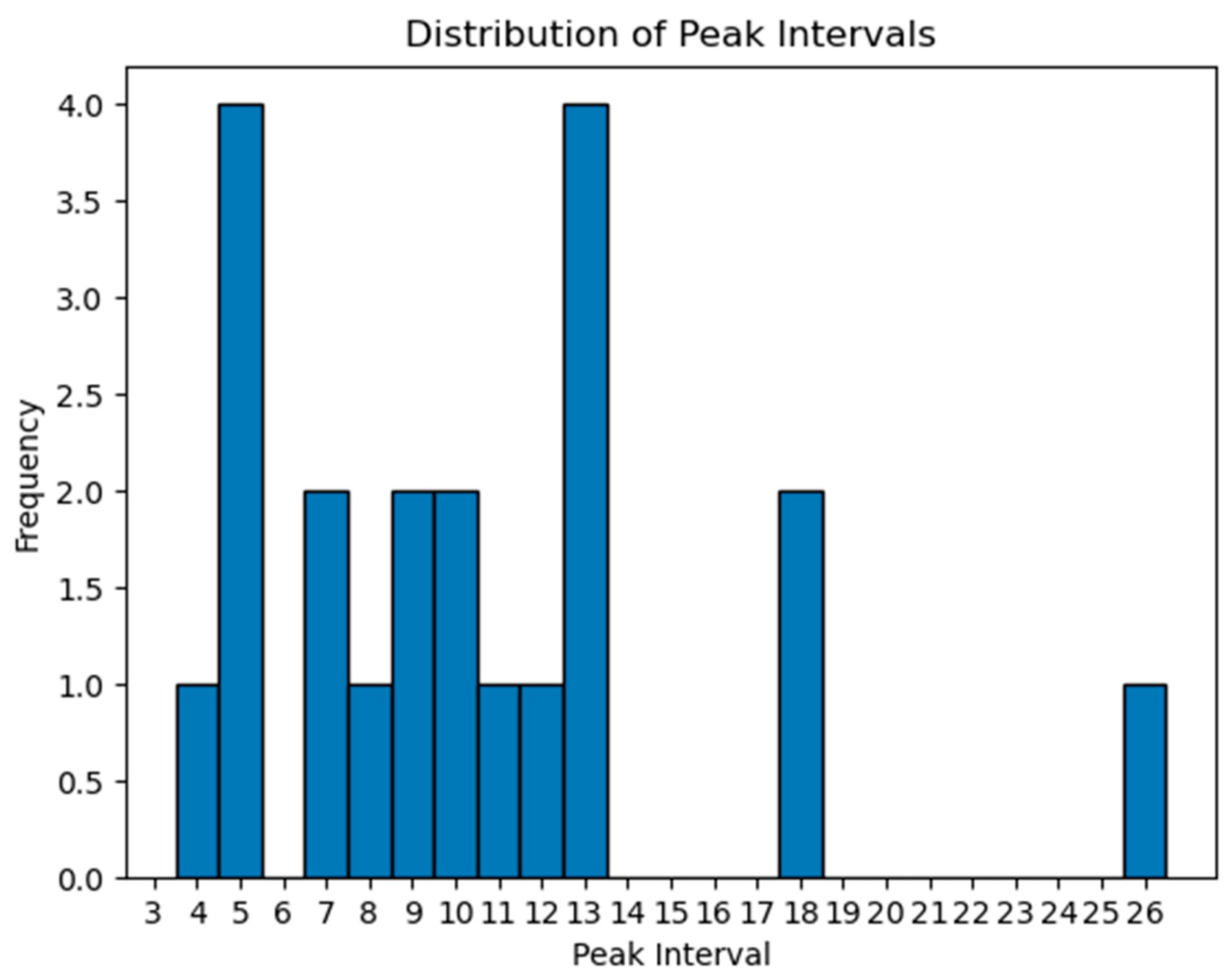
Taking Figure 6a as an example, the histogram of horizontal adjacent peak spacing is shown in Figure 8.
Since abnormal peaks caused by poor DM code image quality will reduce the adjacent peak spacing, an exponential weighted moving average algorithm is used to predict the dividing line spacing after sorting the adjacent peak spacing. The exponential weighted moving average algorithm [40] is a commonly used time series smoothing algorithm for smoothing data and trend analysis. It gives greater weight to recent observations and gradually decreases as the distance between observations and the current time point increases. Through this algorithm, different weights can be assigned to adjacent peak spacings after sorting, reducing the impact of abnormal peaks and predicting dividing line spacings. The calculation formula of the exponential weighted moving average algorithm is shown in Equation (4):
y t = x 0 ,     t = 0 α x t + 1 α y t 1 ,     t > 0 ,
where the position of the current point is t , the value of the current point is x t , the weighted average value at the current time is y t , the weighted average value at the previous time is y t 1 , x 0 represents the value of the first point, and α is the smoothing coefficient, typically between 0 and 1. A larger α gives more weight to the current point x t , making the estimate more responsive to recent changes. A smaller α gives more weight to the previous weighted average y t 1 , resulting in smoother estimates that are less responsive to recent fluctuations.
One must then traverse the detected peaks. If the adjacent peak spacing is less than half of the predicted dividing line spacing, it is considered a peak in the same group. After grouping the peaks, if there is only one peak in a group of peaks, one must directly define the position of that peak as the dividing line position. If there are multiple peaks in a group of peaks and only one maximum peak value, then this maximum peak value is the position where the dividing line position is defined; if multiple peaks have the same maximum value, then the position where the first peak is located is defined as the dividing line position. Finally, one must traverse the dividing line positions. If the adjacent dividing line spacing is greater than twice the predicted dividing line spacing, a dividing line needs to be inserted until the adjacent dividing line spacing is less than twice the predicted dividing line spacing.
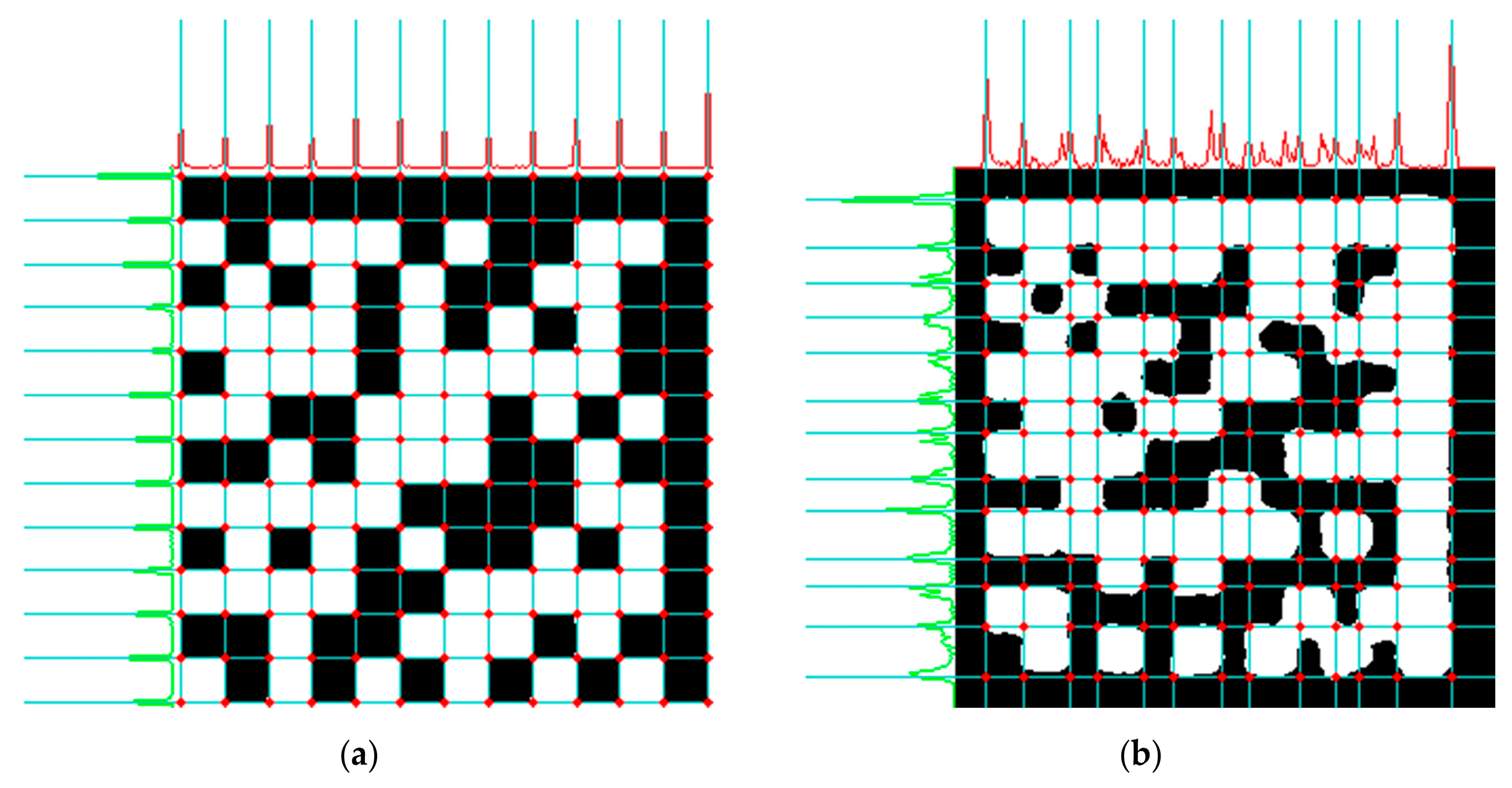
The adaptive sampling grid division effects of Figure 4a and Figure 6a are shown in Figure 9a,b.

4. Binarization Method Based on Grayscale Change Trend

After determining the sampling grid, the grid can be binarized by calculating the proportion of black and white pixels in the grid, calculating the proportion of black and white pixels on the cross-shaped symbol in the center of the grid, and scanning the center pixel of the grid. However, these methods have high requirements for the quality of DM code images. When the background noise or image distortion of DM code images is severe, large errors are likely to occur. This section proposes a binarization method based on the gray change trend. The gray value of unit pixels after iterative division of the grid is calculated to obtain the gray change trend from the periphery to the center of the grid. The LOF algorithm is used to detect outliers in data. After correcting the detected outliers, the local weighted linear regression algorithm is used to predict the gray value of the grid based on this gray change trend and binarize it to convert the DM code image into a data matrix.

4.1. Gray Change Trend

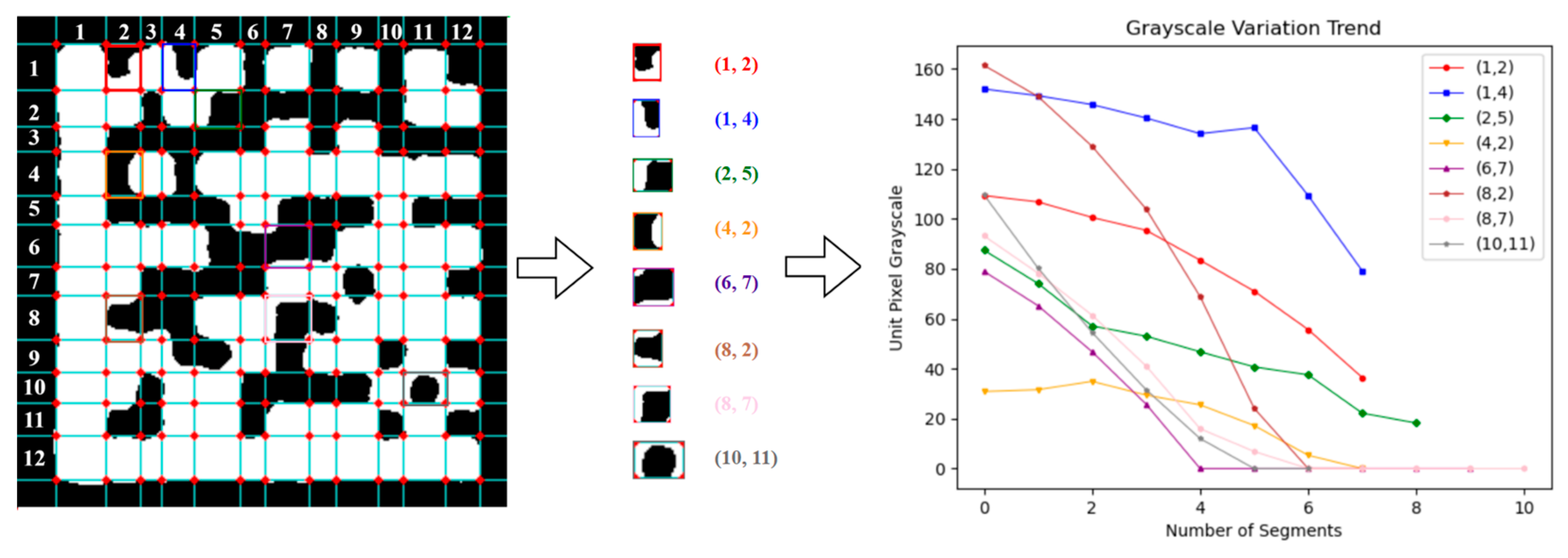
By constructing a mask image [41] and performing an AND operation with each pixel of the DM code image, the target image can be obtained and used to acquire the target grid. The length and width of the target grid are reduced by two pixels in turn for iterative division. The unit pixel gray value of each divided grid is calculated to obtain the gray change trend from the periphery to the center, as shown in Figure 10, where the numbers 1–12 on the first subgraph of Figure 10 represent the row and column indices for locating specific sub-regions, which are used to analyze grayscale variation trends. The pseudocode of this module is shown in Algorithm 1, and its computational complexity is shown in Table 1, where L is the initial size of the grid, x is the number of grids, p is the total number of pixels in the image, and t is the number of gray values per grid.
Algorithm 1. Iterative division of the grid
Input: A list of grids GPL that each contains the four corner coordinates of a grid after partitioning, a binarized black-and-white image BI.
Output: A list of the grayscale distribution trends GVLA for each grid in the grid list.
1: Initialize GVLA as an empty list
2: For each grid_points in GPL:
3:         Initialize an empty list
4:         Get grid_length and grid_width from grid_points
5:         While grid_length > 2 and grid_width > 2:
6:                 Create an empty mask of the same size as BI
7:                 Fill grid_points region in the mask with value 255
8:                 Compute gray_value = mean of pixels in BI inside the mask
9:                 Append gray_value to list
10:                If grid_length > 2 and grid_width > 2:
11:                        Decrease grid_length and grid_width by 2
12:                Else If grid_length ≤ 2 < grid_width:
13:                        Decrease grid_width by 2
14:                Else:
15:                        Decrease grid_length by 2
16:                Update grid_points by shifting corners inward
17:        End While
18:        Append list to GVLA
19: End For
20: Return GVLA

4.2. Outlier Detection and Correction

Outliers are considered to be points that are significantly different from other observations in the dataset or that do not conform to expected normal behavior [42,43]. Traditional outlier detection methods include the statistics-based Pauta criterion [44], the distance-based K-nearest neighbor algorithm [45], and the density-based LOF algorithm [46].
As for the Pauta criterion, it actually does not only require an assumption about the distribution of the data but also requires that the number of points used for outlier detection is large enough. When the number of points is less than or equal to 10, the Pauta criterion fails. To balance the efficiency of the algorithm, the number of divisions for a single grid cannot be too high, as depicted in Figure 9, so it does not meet the requirements of the Pauta criterion for data volume.
As for the distance-based K-nearest neighbor algorithm, it calculates the distance between each point in the dataset and its K-nearest point to detect outliers. However, different k values have a significant impact on the results of this algorithm. If the selected k value is too small, it will cause the outlier detection results of the algorithm to be easily affected by noise. Conversely, it will cause the outlier detection results to be easily affected by distant points. The results obtained by performing outlier detection based on this algorithm may have some flaws.
Density-based outlier detection methods use local density information to detect outliers. The basic idea is to treat points that appear in low-density areas as outliers and points that appear in high-density areas as normal points [47]. The LOF algorithm is the most representative density-based outlier detection method. The core method of the algorithm is to compare the local density deviation between the target point and neighboring points and determine whether the target point is an outlier by calculating the ratio of local density deviation [48]. Since the LOF algorithm incorporates neighboring points while calculating target points, and since the ratio of local density deviation of target points contains information about neighboring points, its accuracy is relatively high. Therefore, this paper uses the LOF algorithm to detect outliers. The relevant definitions and calculation methods of the LOF algorithm are as follows:
  • Distance between sample points. There are many ways to measure the distance between points, and the commonly used distance measurement method can be defined by the Minkowski distance [49]. For a dataset P, the distance between point p and point o is denoted as d p , o , and the Minkowski distance formula is shown in Equation (5):
    d p , o = i = 1 n p i o i q 1 q
    when the value of q in the Minkowski distance expression is 1, it is called the Manhattan distance, which is used to calculate the orthogonal-side distance between two points. When the value of q in the Minkowski distance expression is 2, it is called the Euclidean distance [50], which is used to calculate the straight-line distance between two points in Euclidean space. When the value of q in the Minkowski distance expression tends to infinity, it is called the Chebyshev distance, which is used to calculate the maximum absolute value of the difference between coordinate values. The Chebyshev distance focuses on the maximum deviation in a single dimension and is not sensitive to coordinated changes across multiple directions. The Manhattan distance captures the cumulative horizontal and vertical deviations by summing the differences in each dimension, making it unable to directly reflect the true magnitude of diagonal changes. The Euclidean distance can directly measure the linear distance between two points, providing an accurate measure regardless of whether the deviation occurs horizontally, vertically, or diagonally. This means that the Euclidean distance can capture variations in all directions in DM codes, not just in a certain direction. Therefore, this paper chooses the Euclidean distance as the measurement method for distance.
  • The k-distance. If there are at least k points o C x p in dataset P that do not include p , satisfying d p , o d p , o , at most k−1 points o C x p ; not including p and satisfying d p , o d p , o , then the k-distance d k p of point p refers to the distance between the k-farthest point from p in the dataset and p .
  • The k-distance neighborhood. For dataset P, the k-distance neighborhood of point p is denoted as N k p , and the definition of N k p is shown in Equation (6):
    N k p = o P d p , o d k p .
    In fact, the k-distance neighborhood of point p is a set of points that satisfy special properties. The points in the set satisfy that their distance to point p is less than or equal to the k-distance of point p .
  • Reachability distance. For dataset P, the reachability distance from point p to point o is denoted as r k p , o , and the definition of r k p , o is shown in Equation (7):
    r k p , o = m a x d k p , d p , o .
    The reachability distance from point p to any point is at least equal to the k-distance of point p . If a point belongs to the k-distance neighborhood of point p , then the reachability distance from point p to this point is equal to the k-distance of point p ; if a point does not belong to the k-distance neighborhood of point p , then the reachability distance from point p to this point is equal to the actual distance between the two points.
  • Local reachability density. For dataset P, the local reachability density of point p is denoted as l r d k p , and the definition of l r d k p is shown in Equation (8):
    l r d k p = 1 / o N k p r k p , o N k p ,
    where N k p represents the number of points contained in the k-distance neighborhood of point p . In fact, the local reachability density of point p represents the reciprocal of the average value of the reachability distance from all points in the k-distance neighborhood of point p to point p . When the distance between point p and other points in its k-distance neighborhood is larger, the local reachability density of point p is smaller, indicating that the distribution of point p and its surrounding points is sparser. Conversely, the larger the local reachability density of point p , the denser the distribution of point p and its surrounding points. It should be noted that there is an implicit premise in the definition of local reachability density, i.e., all points in the k-distance neighborhood of point p cannot be duplicate points. This is because if such duplicate points exist, the reachability distance calculated in local reachability density will be zero, causing local reachability density to become infinite.
  • Local outlier factor. For dataset P, the LOF of point p is denoted as L O F k p , and the definition of L O F k p is shown in Equation (9):
    L O F k p = o N k p l r d k o N k p l r d k p ,
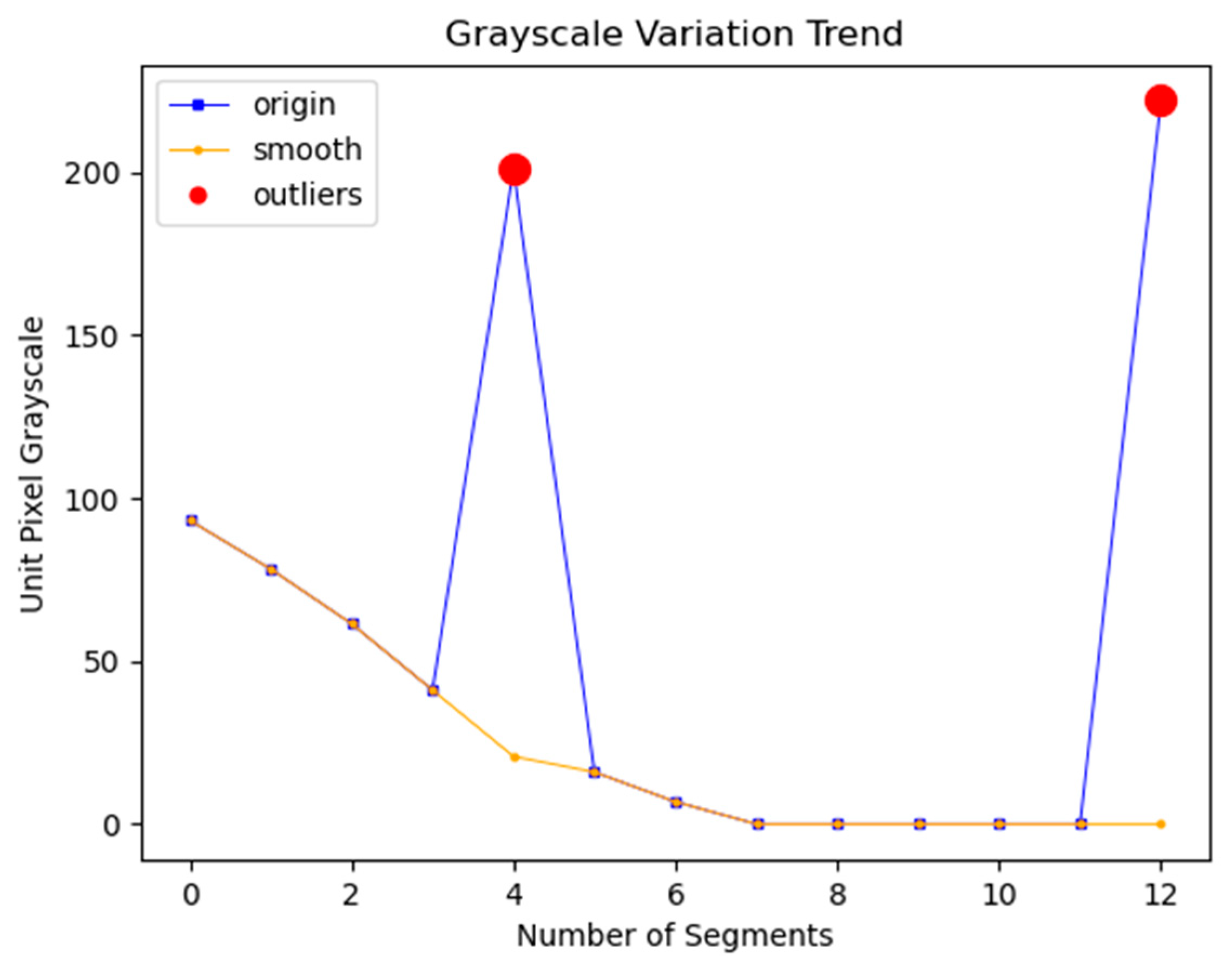
    where the LOF of point p represents the average of the ratio of the local reachability density of the neighborhood points N k p of point p to the local reachability density of point p . If the LOF is less than 1, it means that the local reachability density of point p is higher than that of its neighborhood points, so point p belongs to a dense point. If the LOF is equal to 1, it means that the local reachability density of point p is similar to that of its neighborhood points, so point p and its neighborhood points may belong to the same cluster. If the LOF is greater than 1, it means that the local reachability density of point p is lower than that of its neighborhood points, so point p belongs to an outlier. Based on the LOF algorithm, outliers in the grayscale change trend can be detected. The process of correcting outliers based on the grayscale change trend is as follows: Suppose point r n is an outlier, then the previous point of the outlier is r n 1 , and the next point of the outlier is r n + 1 . The correction value r n of outlier r n is calculated by Equation (10):
    r n = 2 r n + 1 r n + 2 ,     0 < n 2 2 r n 1 r n 2 ,     n > 2 .
    The effect of adding outliers to the grayscale change trend of the grid in the eighth row and seventh column in the first subgraph of Figure 10 and correcting them after outlier detection is shown in Figure 11.

4.3. Locally Weighted Linear Regression

Locally weighted regression is a non-parametric regression method [51]. In traditional linear regression methods, it is often necessary to assume the distribution family of the data source and select an appropriate model for parameter estimation. However, in practical applications, the distribution of the data is unknown and cannot fully satisfy a single specified distribution as a whole. Due to the complexity of the overall data distribution, local statistics can be used to simplify it. Locally weighted regression can fit a complex global model with a simple local model assumption [52]. The basic idea of locally weighted regression is to assign different weights to training samples based on the distance between point x to be predicted and the training samples, so that training samples closer to point x have larger weights, thereby learning local information about the data differently. In local regression methods, the most commonly used local model is still linear. Local ridge regression adds a regularization term based on local linear regression, making the model more robust to noise, but it does not help improve reconstruction accuracy [53]. Therefore, this paper proposes to use a locally weighted linear regression algorithm to predict the gray value of the grid based on this gray change trend and binarize it to convert the DM code image into a data matrix.
For dataset S = x i , y i , x i R , y i R , i = 1,2 , , N , the general form of the locally weighted model can be represented by Equation (11) as a weighted minimization problem [51]:
m i n i = 1 N L f x i , β , y i K h d x i , x ,
where x i and y i are the number of segments in the training set and their corresponding unit pixel gray values. x is the test sample to be predicted, and β is the local model parameter to be solved by the minimization problem. f x , β is the locally weighted prediction result of x , d x i , x is the distance between data point x and test point x i , and the Euclidean distance is used in this paper. L · is the loss function and K h · is the weighting or kernel function.
In regression problems, squared loss functions or absolute value loss functions are commonly used. In practical problems, for ease of solution, squared loss functions are generally chosen. That is, Equation (11) can be specifically represented by Equation (12):
m i n i = 1 N f x i , β y i 2 K h d x i , x .
In this paper, for the discrete dataset S, the Wang–Ryzin kernel function is used to calculate the weights. The kernel function K h d x i , x is denoted as ω i x , and the expression of the Wang–Ryzin kernel function [54] is shown in Equation (13):
ω i x = 1 h ,   x = x i 1 h 2 h x i x ,   x x i ,
where h represents the bandwidth, which controls the speed of weight decay. Choosing an appropriate bandwidth is crucial for the performance of the kernel function. In this paper, the optimal bandwidth parameter is selected through leave-one-out cross-validation. The calculation formula of the leave-one-out cross-validation function [55] is shown in Equation (14):
C V h = 1 n i = 1 N y i g ^ i x i 2 ,
where g ^ i x i is the estimated value of g x i obtained based on the leave-one-out method.
Considering that the local model in this paper is a linear model, f x , β can be represented by Equation (15):
f x , β = β T x .
Substituting Equations (15) and (13) into Equation (12), the weighted minimization problem is represented by Equation (16) [56]:
m i n i = 1 N ω i x β T x y i 2 .
Equation (16) is rearranged into matrix form as shown in Equation (17):
m i n X β Y T W X β Y ,
where X represents the matrix of input training data and Y is the estimated output vector. W is the diagonal matrix of weights, specifically shown in Equation (18) [57]:
W = ω 1 x 0 0 0 ω 2 x 0 0 0 ω N x .
Taking the partial derivative of the objective function in Equation (17) with respect to parameter β and setting the partial derivative to zero, the solution to the corresponding weighted least squares problem is as follows:
X β Y T W X β Y β = 2 X T W X β 2 X T W Y = 0 ,
β = X T W X 1 X T W Y .
Therefore, for test sample x, its locally weighted linear regression prediction result is as follows:
y ^ = Y T W X X T W X 1 x
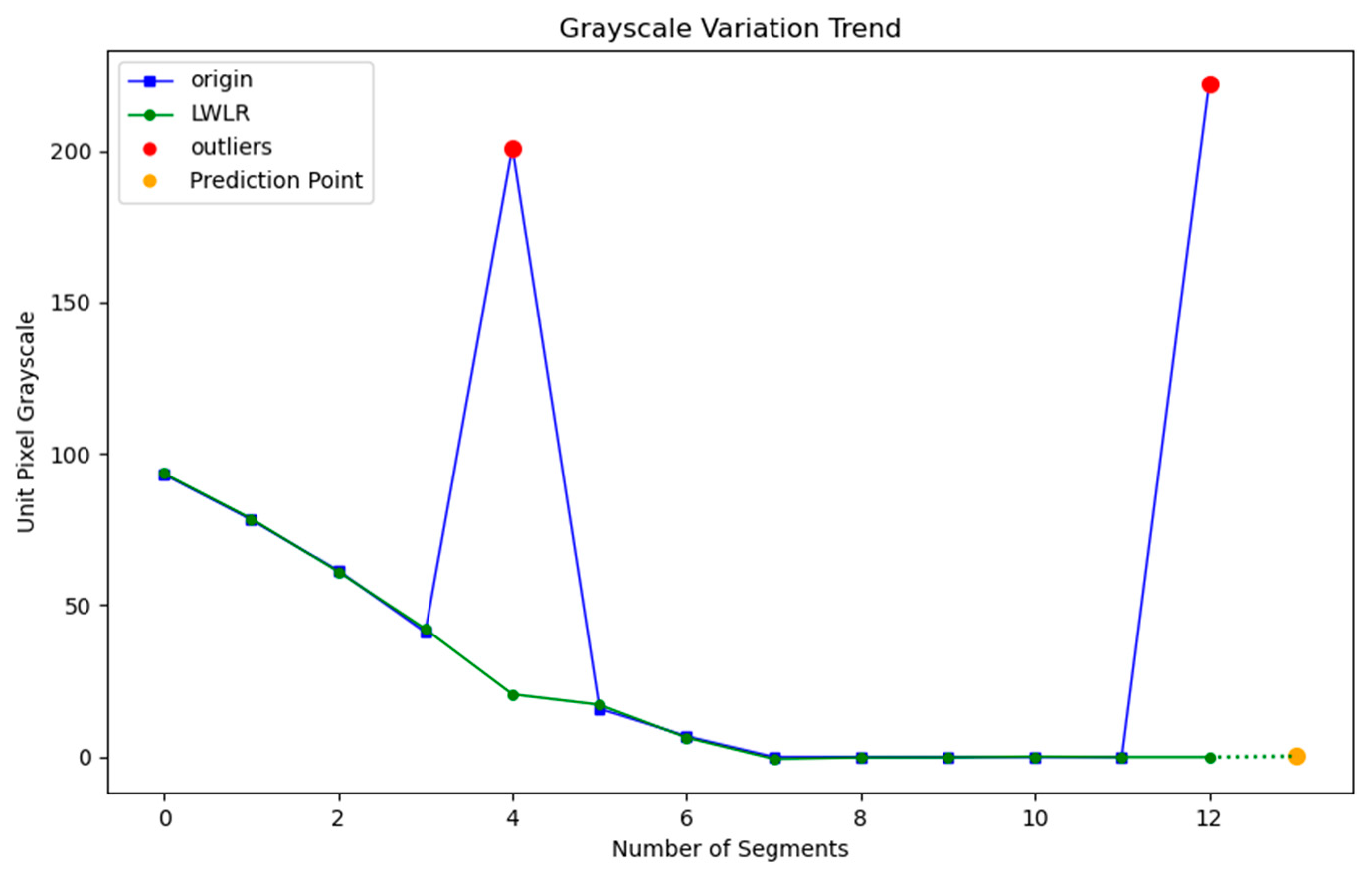
Taking Figure 11 as an example, after detecting and correcting outliers based on the gray change trend, the predicted gray values using the locally weighted linear regression algorithm are shown in Figure 12.
After obtaining the predicted gray values, we set the threshold to T = 128 and binarize the grid to convert the DM code image into a data matrix, as depicted in Figure 13. The pseudocode of predicting gray values and converting the DM code into a data matrix is shown in Algorithm 2, and its computational complexity is shown in Table 2, where m is the number of grayscale trend lists and n is the length of each grayscale trend list.
Algorithm 2. Grayscale prediction and output of data matrix
Input: A list of the grayscale distribution trends GVLA from Algorithm 1.
Output: A decoded data matrix DM.
1: Initialize an empty list
2: For each gray_trend_list in GVLA:
3:           Create an array x of indices from 0 to len(gray_trend_list) − 1
4:           Convert gray_trend_list to a numpy array y
5:           Apply Local Outlier Factor (LOF) to detect outliers in y
6:           Identify outlier_indices where LOF = −1
7:           For each outlier_idx in outlier_indices:
8:                      If outlier_idx is at start or end, apply smoothing based on neighbors
9:           End For
10:          Fit Kernel Regression model on smoothed y with x
11:          Calculate predicted gray value for next point
12:          If predicted gray value > 128:
13:                     Set predicted value to 255 (black)
14:          Else:
15:                      Set predicted value to 0 (white)
16:          Append predicted value to list

17: End For# Post-processing after obtaining the predicted gray values
18: Reshape list into a 2D array
19: Modify the first row to have alternating 0 and 255 values
20: Modify the last column to have alternating 255 and 0 values
21: Set the first column and the last row to 0
22: Return DM

5. Experiments and Result Analysis

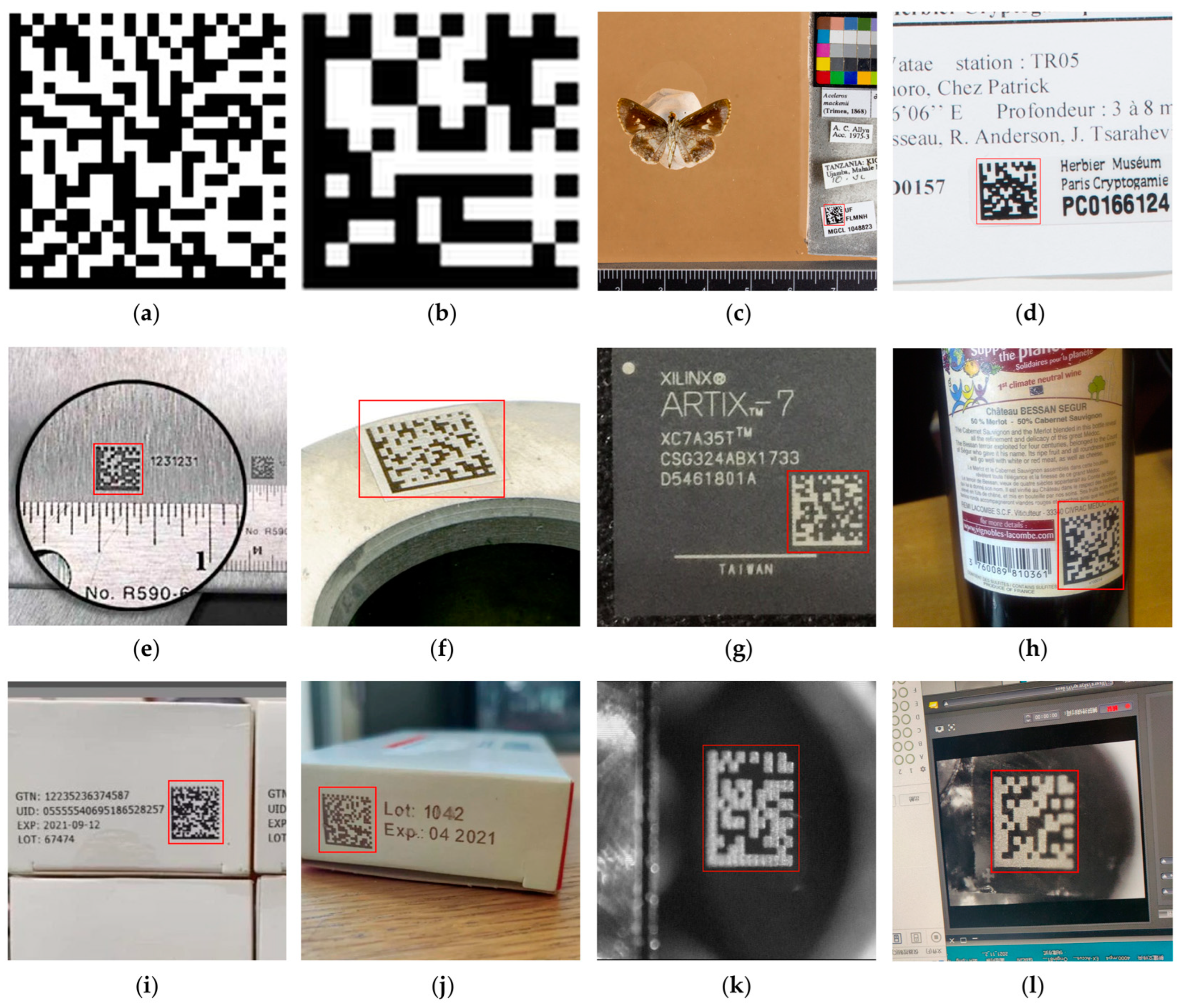
To verify the performance of the above algorithm, we conducted experiments on the problems of DM code image blur, wear, corrosion, geometric distortion, and strong background interference in practical application scenarios and present 12 representative experimental results in this paper. After that, we prepared two types of datasets, including 20 standard 12 × 12 DM code images, and 10 DM code labels on butterfly specimens, to compare with other DM code decoding algorithms with respect to resolution, anti-noise, anti-distortion, execution time, and memory consumption.
Figure 14a–l are twelve original test images. Figure 14a,b are standard 24 × 24 and 12 × 12 DM code images; Figure 14c is a close-up image of a butterfly specimen label with a DM code, where the size of the DM code is small. Figure 14d is an image of a DM code label with printing issues, leading to image distortion, which affects its readability; Figure 14e,f are images of a mechanical tool and a component with DM codes etched onto the metallic surface. Due to the small size of Figure 14e and the shooting inclination of Figure 14f, the resolution is low, affecting its legibility. Figure 14g is a DM code image etched on a chip. The chip is tiny and the DM code image is even smaller, resulting in low resolution and blur of the DM code image. Figure 14h is a DM code label on a bottle, where the distortion of the DM code and the poor lighting add to the difficulty of decoding. Figure 14i,j are the DM code labels on medicine boxes, where stains and glue marks on the surface of the boxes affect decoding. Figure 14k,l are barcode labels on microbial mass spectrometer target plates; due to the poor lighting and tilted shooting angle, there is strong background interference and image distortion.
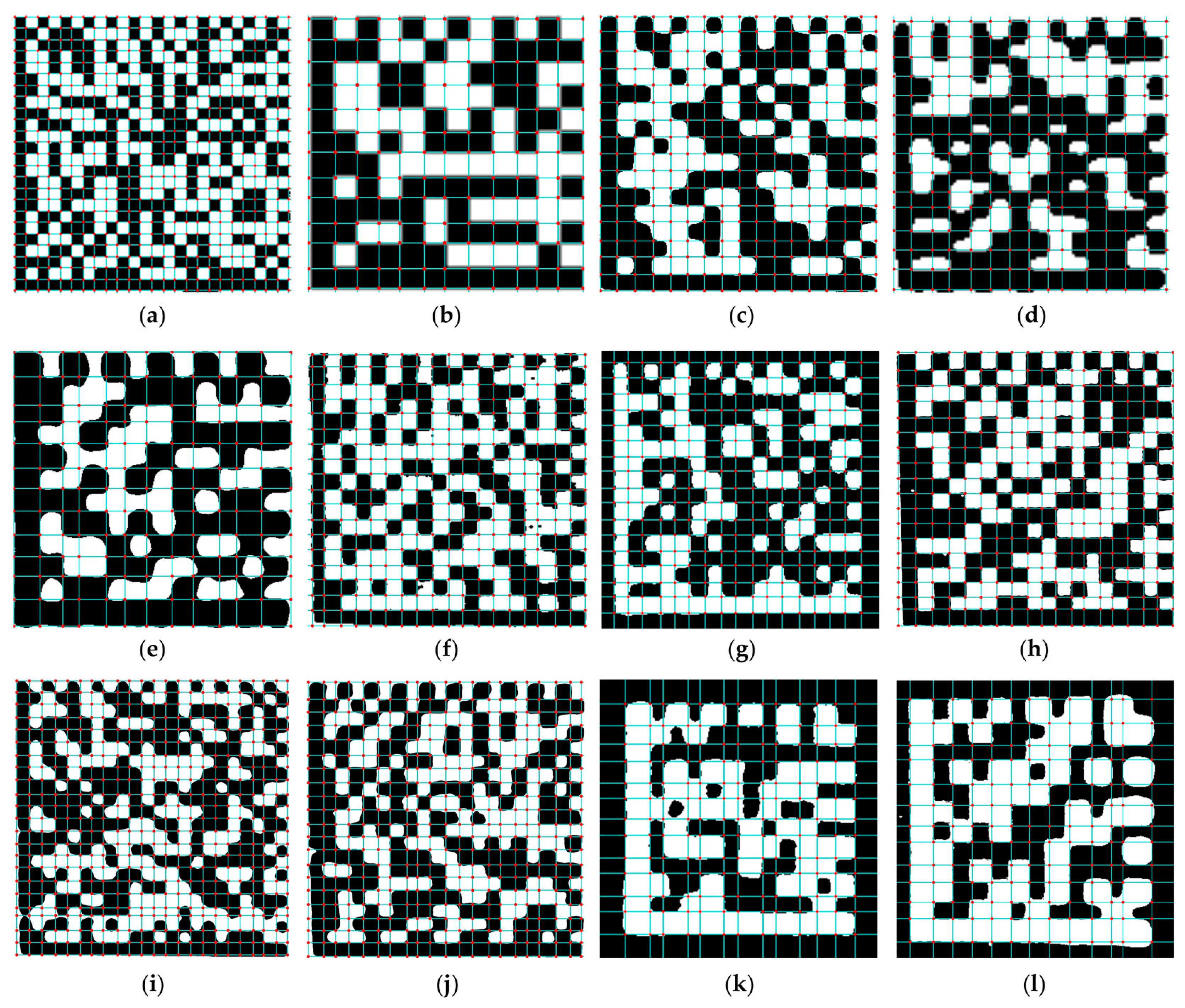
Figure 15a–l are the experimental results of DM code image sampling grid division. The results show that the proposed adaptive sampling grid division method is effective and accurate. Figure 15c,e,g,i show that the adaptive sampling grid division method has high accuracy for small-size and low-resolution DM code images; Figure 15f,h,j–l show that even under distortion conditions or harsh lighting, the proposed method can accurately divide the sampling grid and has good robustness against interference from complex backgrounds. Figure 15d highlights this method’s effectiveness in handling image deformation caused by printing issues.
Based on Figure 15a–l, experiments were conducted on binarization based on the grid grayscale change trend. To facilitate observation of the experimental results, the data matrix generated by DM code images was visualized, and the experimental results were obtained successively, as shown in Figure 16a–l. Among them, dark modules and light modules represent binary “1” and “0”.
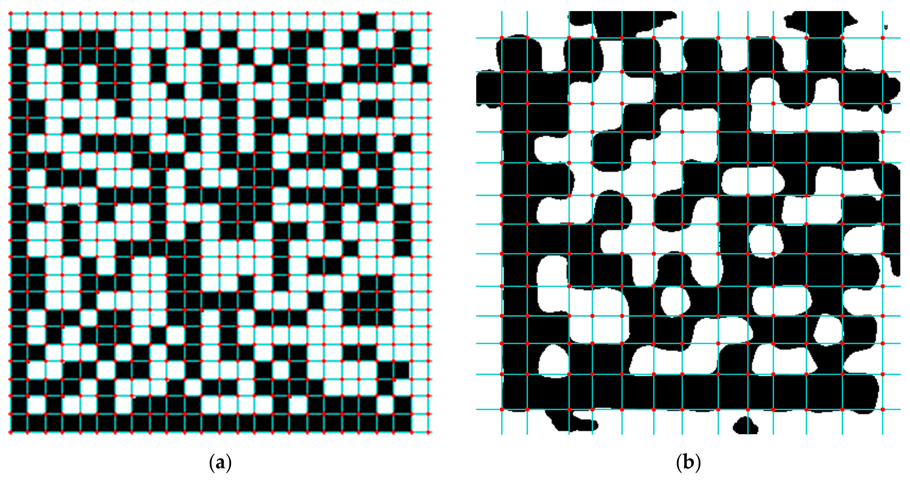
When using popular DM code decoding open-source libraries libdmtx [58] and zxing [59], taking Figure 14a,e as examples, where Figure 14e requires cropping before processing, since libdmtx and zxing both define the size of data modules based on finder patterns, if they are damaged, this will lead to failure of DM code decoding. However, through the adaptive sampling grid division method proposed in this paper, as long as there is one module left on the rows and columns used by finder patterns to define data module size, the sampling grid can be accurately divided, as illustrated in Figure 17a,b, and after rebuilding finder patterns, DM code information can be parsed through libdmtx and zxing.
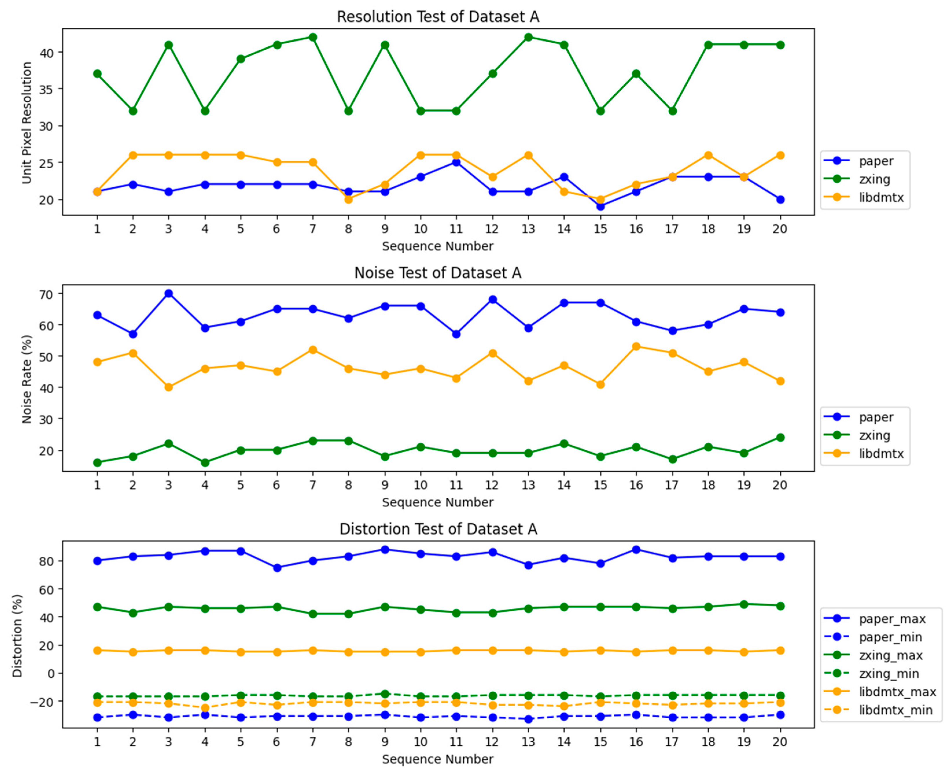
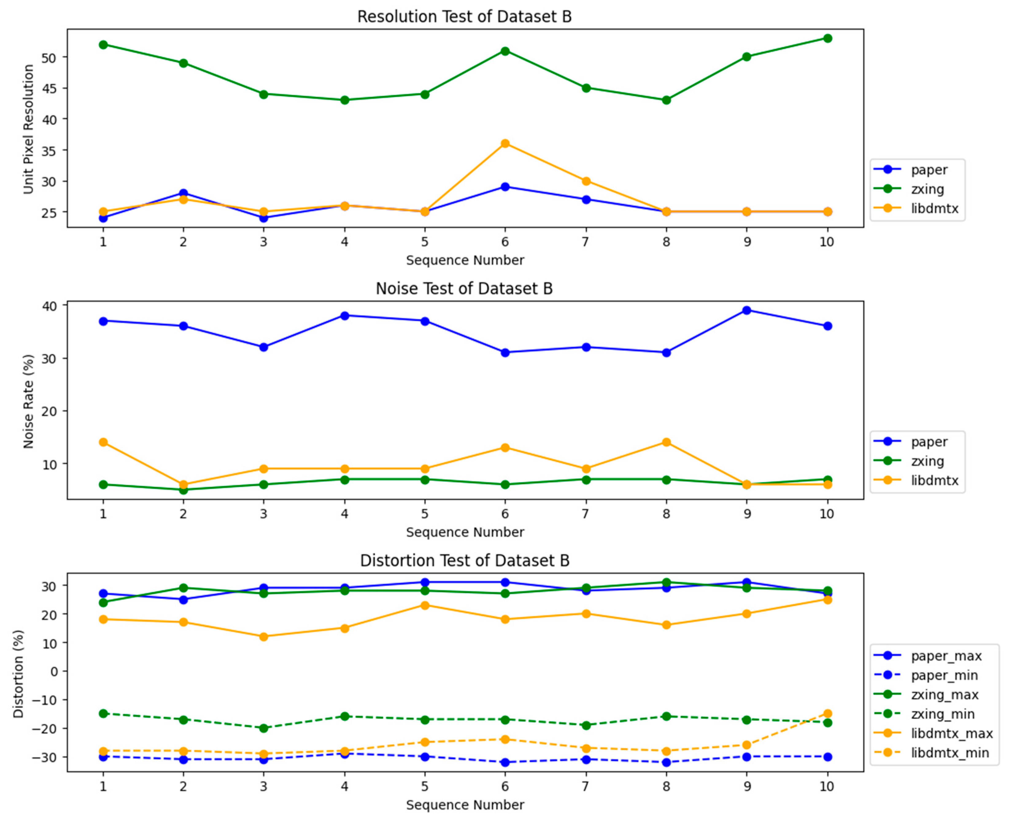
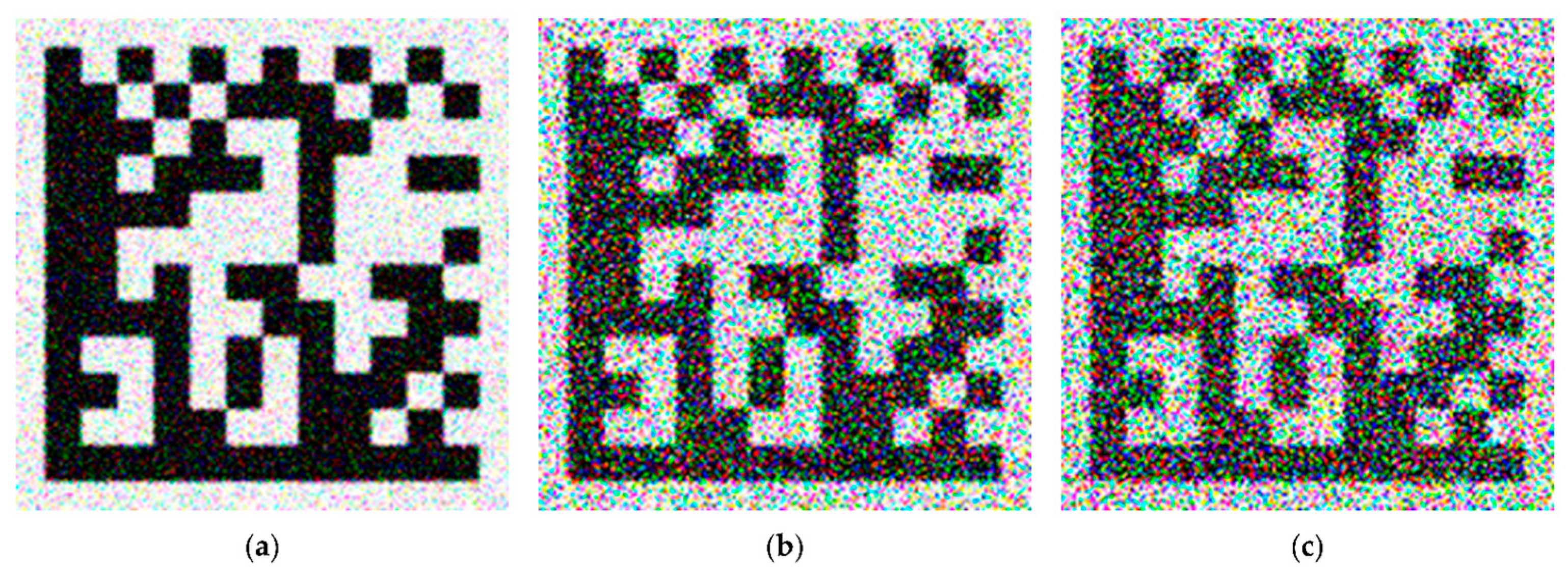
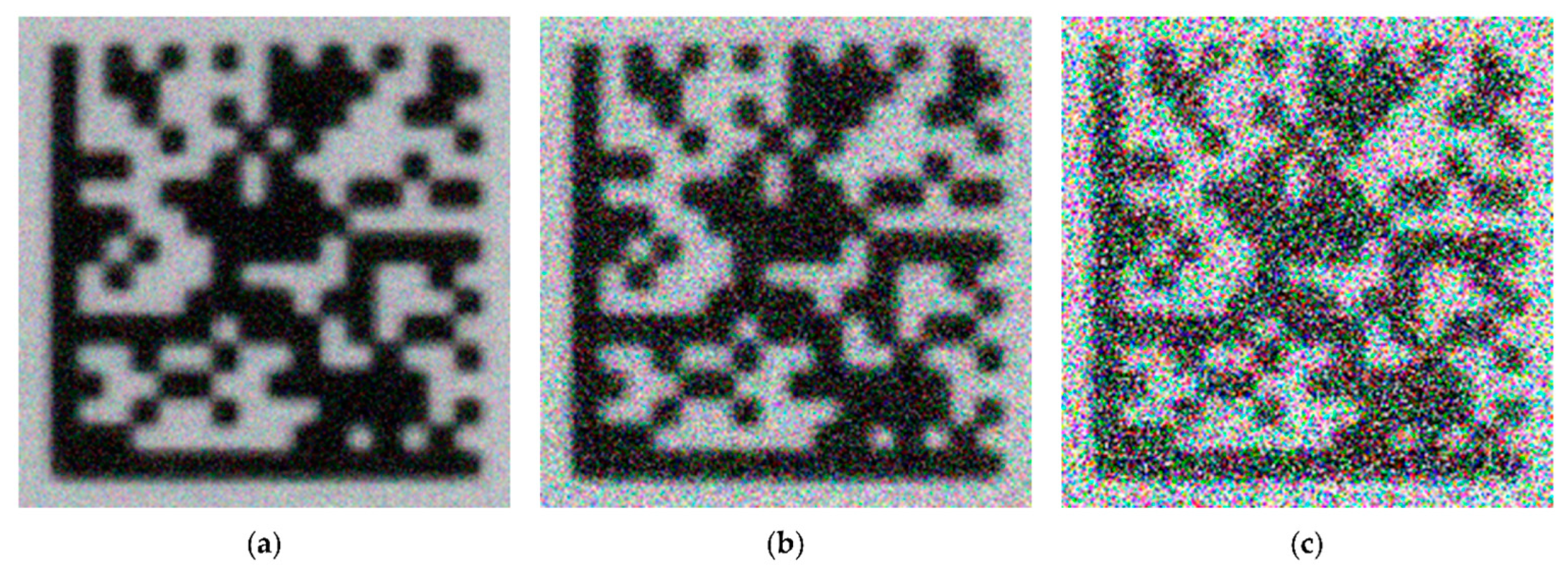
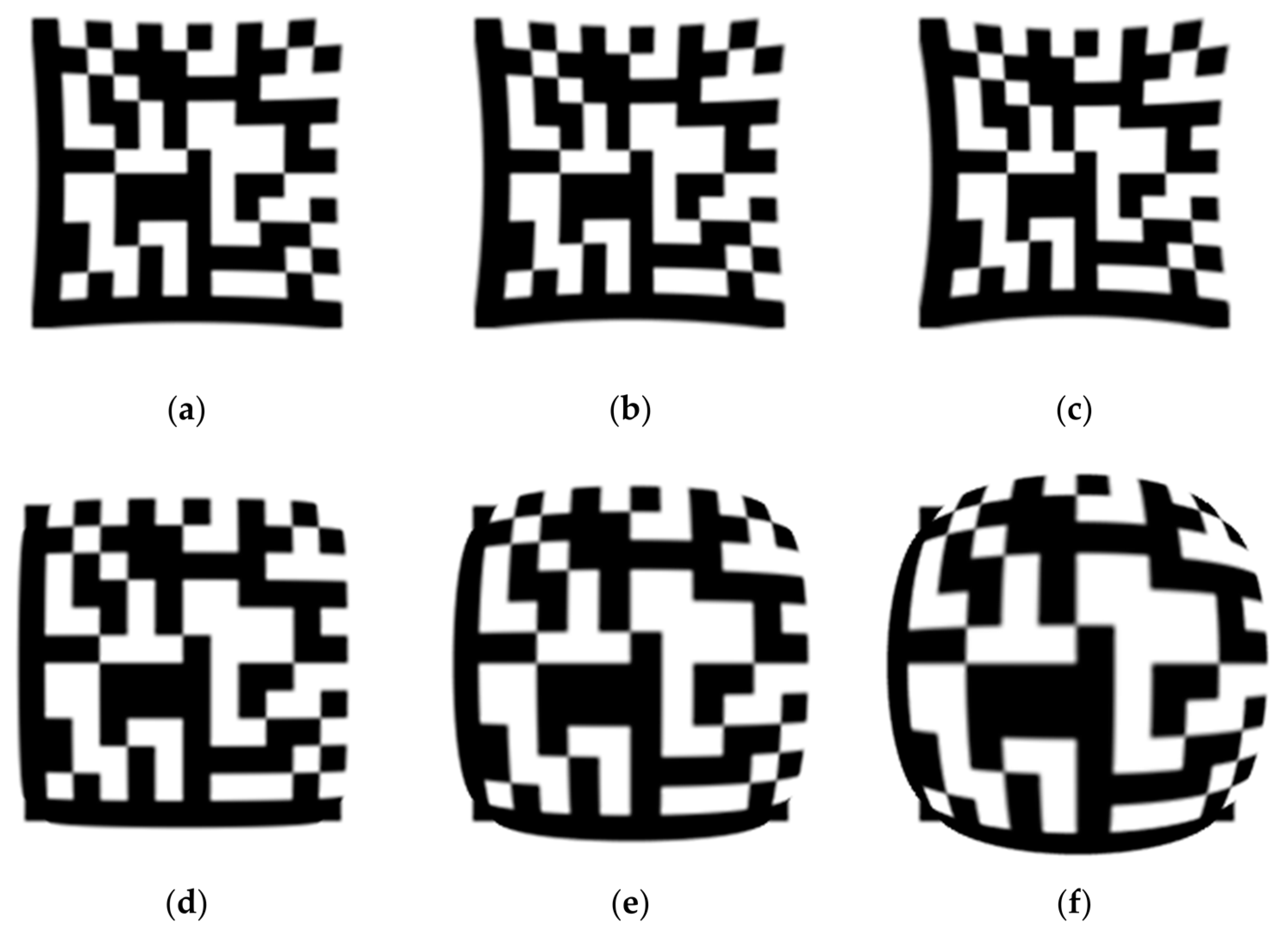
This paper takes two types of datasets, including 20 standard 12 × 12 DM code images as Dataset A and 10 DM code labels on butterfly specimens as Dataset B. To facilitate better recognition of the DM codes, the images of butterfly specimens need to be cropped before processing. Compared with popular DM code decoding open-source libraries libdmtx and zxing, this algorithm was evaluated in terms of resolution, anti-noise, and anti-distortion, with the experimental results presented in Figure 18 and Figure 19. In addition, this paper also compares the execution time and memory consumption of the proposed algorithm with libdmtx and zxing using DM code images from Datasets A and B without added noise or distortion, with the results shown in Table 3. Among them, the experimental conditions for testing resolution are as follows: converting all of the DM code images in both Datasets A and B into data matrices and constructing all of them into DM code images of different pixel sizes to measure the minimum size that can be recognized. The experimental conditions for testing anti-noise are as follows: cropping the DM code images in Dataset A, and then converting all of the DM code images in both Datasets A and B into data matrices and constructing them into DM code images of size 200 × 200 pixels. A specified proportion of Gaussian noise was randomly added. Taking continuous failure to recognize noise 50 times as the judgment standard, the maximum proportion of Gaussian noise that can be recognized was measured. The DM code images after adding different proportions of Gaussian noise to Datasets A and B are depicted in Figure 20 and Figure 21, respectively. The experimental conditions for testing anti-distortion are as follows: converting all of the DM code images in both Datasets A and B into data matrices and constructing them into DM code images of size 200 × 200 pixels. A specified proportion of spherical distortion was added. Taking continuous failure to recognize distortion 50 times as the judgment standard, the maximum proportion of spherical distortion that can be recognized was measured. The DM code images after adding different proportions of spherical distortion to Datasets A and B are presented in Figure 22 and Figure 23, respectively.
The experimental results show that this algorithm can accurately convert the DM code into a data matrix when facing problems such as DM code image blur, wear, corrosion, geometric distortion, and strong background interference in practical application scenarios, improving decoding ability in complex environments. Compared with popular DM code decoding open-source libraries libdmtx and zxing, it also has good performance in terms of resolution, anti-noise, and anti-distortion. However, it should be noted that the proposed algorithm, due to its complex processing steps including adaptive grid division, outlier detection and correction, and locally weighted linear regression, requires more computational resources than traditional decoding libraries. Experimental comparison shows that the average execution time of this algorithm is 14.971 s and average memory consumption is 329.454 KB, whereas libdmtx and zxing exhibit significantly faster decoding speeds and lower memory usage (0.004 s and 60.364 KB for libdmtx, and 0.356 s and 6.909 KB for zxing). This indicates that while the proposed method offers superior robustness under challenging conditions, it is more suitable for scenarios where decoding accuracy is prioritized over speed and resource consumption.

6. Conclusions

This paper proposes a DM code recognition algorithm based on the coarse positioning of images. The algorithm uses a projection algorithm and an exponential weighted moving average model to convert two-dimensional barcodes into one-dimensional waveforms for analysis and corrects abnormal segmentation lines to achieve adaptive division of sampling grids. After dividing the sampling grid, combined with the LOF algorithm and local weighted linear regression algorithm, according to the grayscale change trend of the sampling grid, the grayscale value of the grid is predicted and binarization is performed to achieve conversion from a DM code image to a data matrix.
Compared with traditional algorithms, this algorithm can effectively divide the sampling grid of DM codes whose finder patterns are polluted or missing and has been optimized for problems such as DM code image blur, wear, corrosion, geometric distortion, and strong background interference in practical application scenarios. It reduces the quality requirements for DM code images and improves the robustness of DM code recognition in complex environments.
Although this algorithm has higher robustness in DM code recognition in complex environments, for DM code images with clean backgrounds, less pollution, and high image quality, this algorithm is slightly cumbersome and has low computational efficiency. Therefore, the best application object of this algorithm is DM code images with a high-pollution background or low image quality, as it can be used as an alternative plan after traditional algorithm recognition fails. Future work on this algorithm aims to focus on improving its efficiency, such as by incorporating machine learning-based optimization techniques to reduce processing time and memory consumption. Furthermore, improving its computational efficiency, expanding its application to real-time systems, and exploring its integration with automation processes in industries like logistics, manufacturing, and healthcare could bring significant benefits in environments where image quality is often compromised.
The next step will involve testing the algorithm with a broader range of real-world data and investigating the possibility of applying the method to other types of two-dimensional barcodes, paving the way for further optimization and real-world deployment.

Author Contributions

Conceptualization, L.H., G.Z. and Z.C. (Zhiwei Chen); methodology, L.H. and G.Z.; software, L.H. and G.Z.; validation, L.H. and G.Z.; formal analysis, L.H., G.Z. and Z.C. (Zhiwei Chen); investigation, L.H. and G.Z.; resources, Z.C. (Zhiwei Chen) and Z.C. (Zhong Chen); data curation, G.Z.; writing—original draft preparation, L.H.; writing—review and editing, G.Z. and Z.C. (Zhiwei Chen); visualization, L.H. and G.Z.; supervision, Z.C. (Zhiwei Chen) and Z.C. (Zhong Chen) All authors have read and agreed to the published version of the manuscript.

Funding

This research received no external funding.

Data Availability Statement

The archived version of the code and the data presented in this article are publicly available in the GitHub repository at https://github.com/LingyHu/DataMatrix (accessed on 21 February 2025).

Conflicts of Interest

The authors declare no conflicts of interest.

References

  1. Martínez-Moreno, J.; Marcén, P.G.; Torcal, R.M. Data matrix (DM) codes: A technological process for the management of the archaeological record. J. Cult. Heritage 2011, 12, 134–139. [Google Scholar] [CrossRef]
  2. ISO/IEC. Information Technology—Automatic Identification and Data Capture Techniques—Data Matrix Bar Code Symbology Specification; International Organization for Standardization: Geneva, Switzerland, 2006. [Google Scholar]
  3. Dai, Y.; Liu, L.; Song, W.; Du, C.; Zhao, X. The realization of identification method for DataMatrix code. In Proceedings of the 2017 International Conference on Progress in Informatics and Computing (PIC), Nanjing, China, 15–17 December 2017; pp. 410–414. [Google Scholar] [CrossRef]
  4. Dita, I.-C.; Otesteanu, M.; Quint, F. Scanning of industrial data matrix codes in non orthogonal view angle cases. In Proceedings of the 6th Euro American Conference on Telematics and Information Systems, Valencia, Spain, 23–25 May 2012; Association for Computing Machinery: Valencia, Spain, 2012; pp. 363–366. [Google Scholar] [CrossRef]
  5. Kulshreshtha, R.; Kamboj, A.; Singh, S. Decoding robustness performance comparison for QR and data matrix code. In Proceedings of the Second International Conference on Computational Science, Engineering and Information Technology, Coimbatore, India, 26–28 October 2012; Association for Computing Machinery: Coimbatore UNK, India, 2012; pp. 722–731. [Google Scholar] [CrossRef]
  6. Moss, C.; Chakrabarti, S.; Scott, D.W. Parts quality management: Direct part marking of data matrix symbol for mission assurance. In Proceedings of the 2013 IEEE Aerospace Conference, Big Sky, MT, USA, 2–9 March 2013; pp. 1–12. [Google Scholar] [CrossRef]
  7. Karrach, L.; Pivarčiová, E. Recognition of Data Matrix codes in images and their applications in Production Processes. Manag. Syst. Prod. Eng. 2020, 28, 154–161. [Google Scholar] [CrossRef]
  8. Li, J.; Su, G.; Liu, L. Research on DPM technology standardization status quo and development suggestion. Stand. Sci. 2009, 32–35. [Google Scholar]
  9. Czerwińska, K.; Pacana, A. Analysis of the implementation of the identification system for directly marked parts-Data Matrix code. Prod. Eng. Arch. 2019, 23, 22–26. [Google Scholar] [CrossRef]
  10. Iwabuchi, S.; Kakazu, Y.; Koh, J.-Y.; Harata, N.C. Evaluation of the effectiveness of Gaussian filtering in distinguishing punctate synaptic signals from background noise during image analysis. J. Neurosci. Methods 2014, 223, 92–113. [Google Scholar] [CrossRef]
  11. Green, O. Efficient Scalable Median Filtering Using Histogram-Based Operations. IEEE Trans. Image Process. 2018, 27, 2217–2228. [Google Scholar] [CrossRef]
  12. Xiao, H.; Guo, B.; Zhang, H.; Li, C. A Parallel Algorithm of Image Mean Filtering Based on OpenCL. IEEE Access 2021, 9, 65001–65016. [Google Scholar] [CrossRef]
  13. Otsu, N. A threshold selection method from gray-level histograms. IEEE Trans. Syst. Man Cybern. 1979, 9, 62–66. [Google Scholar] [CrossRef]
  14. Yang, Y.; Zhang, Z. A novel local threshold binarization method for QR image. In Proceedings of the International Conference on Automatic Control and Artificial Intelligence (ACAI 2012), Xiamen, China, 3–5 March 2012; pp. 224–227. [Google Scholar] [CrossRef]
  15. Wang, Q. Segmentation of maximum entropy threshold based on gradient boundary control. J. Comput. Appl. 2011, 31, 1030–1032+1120. [Google Scholar] [CrossRef]
  16. Qiang, F. Application of Bernsen method in the field of character segmentation. Heilongjiang Sci. Technol. Inf. 2014, 144–145. [Google Scholar] [CrossRef]
  17. Kim, T.-S.; Park, K.-A.; Lee, M.-S.; Park, J.-J.; Hong, S.; Kim, K.-L.; Chang, E. Application of Bimodal Histogram Method to Oil Spill Detection from a Satellite Synthetic Aperture Radar Image. Korean J. Remote. Sens. 2013, 29, 645–655. [Google Scholar] [CrossRef]
  18. Li, D.; Guo, H.; Tian, J.; Tian, Y. An improved method of locating L-edges in DataMatrix codes. J. Shenzhen Univ. (Sci. Eng.) 2018, 35, 151–157. [Google Scholar] [CrossRef]
  19. Chen, W.; Zhang, X. Improved edge detecting algorithm of mathematical morphology. In Proceedings of the in 2010 International Conference on Machine Vision and Human-Machine Interface, Kaifeng, China, 24–25 April 2010; IEEE: Piscataway, NJ, USA, 2010; pp. 199–202. [Google Scholar] [CrossRef]
  20. Lingling, L.; Yaoquan, Y.; Tao, G. The detection and realization of Data Matrix code by accurate locating. Int. J. Adv. Pervasive Ubiquitous Comput. 2014, 6, 35–42. [Google Scholar] [CrossRef]
  21. Michael, D. Multithreaded two-pass connected components labelling and particle analysis in ImageJ. R. Soc. Open Sci. 2021, 8, 201784. [Google Scholar] [CrossRef]
  22. Karrach, L.; Pivarčiová, E.; Nikitin, Y.R. Comparing the impact of different cameras and image resolution to recognize the data matrix codes. J. Electr. Eng. 2018, 69, 286–292. [Google Scholar] [CrossRef]
  23. Chen, W.; Chen, B. Extraction technology of 2-D barcode under complicated background. J. Xi’an Univ. Posts Telecommun. 2014, 19, 48–51. [Google Scholar]
  24. Zhu, C.; Ge, D.-Y.; Yao, X.-F.; Xiang, W.-J.; Li, J.; Li, Y.-X. Zebra-crossing detection based on cascaded Hough transform principle and vanishing point characteristics. Open Comput. Sci. 2023, 13, 20220260. [Google Scholar] [CrossRef]
  25. Wu, Q.; He, Y.; Luo, Y. Research on QR code image processing on the LED screen. In Proceedings of the International Conference on Optics and Image Processing (ICOIP 2021), Guilin, China, 4–6 June 2021; Volume 11915. [Google Scholar] [CrossRef]
  26. Wang, L.; Chen, Z.; Chen, S.; Chen, X. An improved algorithm of simple polygon convex hull. Comput. Eng. 2007, 33, 200–201. [Google Scholar]
  27. Solomon, C.; Breckon, T. Fundamentals of Digital Image Processing: A Practical Approach with Examples in Matlab. Available online: https://onlinelibrary.wiley.com/doi/book/10.1002/9780470689776 (accessed on 21 February 2025).
  28. Min, Q.; Zhang, X.; Li, D.; Fan, Y. The review of algorithms to correct barrel distortion image. Adv. Mater. Res. 2012, 628, 403–409. [Google Scholar] [CrossRef]
  29. Yuan, J.; Suen, C.Y. An optimal algorithm for detecting straight lines in chain codes. In Proceedings of the 11th IAPR International Conference on Pattern Recognition. Vol. III. Conference C: Image, Speech and Signal Analysis, The Hague, The Netherlands, 30 August–3 September 1992; pp. 692–695. [Google Scholar] [CrossRef]
  30. Greene, N.; Heckbert, P.S. Creating Raster Omnimax Images from Multiple Perspective Views Using the Elliptical Weighted Average Filter. IEEE Comput. Graph. Appl. 1986, 6, 21–27. [Google Scholar] [CrossRef]
  31. Kwon, H. AudioGuard: Speech Recognition System Robust against Optimized Audio Adversarial Examples. Multimedia Tools Appl. 2024, 83, 57943–57962. [Google Scholar] [CrossRef]
  32. Rosenfeld, A.; Pfaltz, J.L. Sequential Operations in Digital Picture Processing. J. ACM 1966, 13, 471–494. [Google Scholar] [CrossRef]
  33. Liao, L.; Li, J.; Lu, C. Data Extraction Method for Industrial Data Matrix Codes Based on Local Adjacent Modules Structure. Appl. Sci. 2022, 12, 2291. [Google Scholar] [CrossRef]
  34. Wang, W.; He, W.; Lei, L.; Li, W.; Guo, G. Accurate location of polluted DataMatrix code from multiple views. J. Comput.-Aided Des. Comput. Graph. 2013, 25, 1345–1353. [Google Scholar] [CrossRef]
  35. Liu, Z.; Zheng, H.; Cai, W. Research on Two-Dimensional Bar Code Positioning Approach Based on Convex Hull Algorithm. In Proceedings of the International Conference on Digital Image Processing, Bangkok, Thailand, 7–9 March 2009; pp. 177–180. [Google Scholar] [CrossRef]
  36. Hu, D.; Tan, H.; Chen, X. The application of Radon transform in 2D barcode image recognition. Wuhan Univ. J. (Nat. Sci. Ed.) 2005, 51, 584–588. [Google Scholar] [CrossRef]
  37. Lu, X.; Bao, X.; Shen, Y. Data Matrix code positioning and recognition in complex background of PCB board. J. Hubei Minzu Univ. (Nat. Sci. Ed.) 2019, 37, 296–299+303. [Google Scholar]
  38. Lv, H.; Shan, P.; Shi, H.; Zhao, L. An adaptive bilateral filtering method based on improved convolution kernel used for infrared image enhancement. Signal, Image Video Process. 2022, 16, 2231–2237. [Google Scholar] [CrossRef]
  39. Xiang, A.; Qin, J.; Cai, H. A new method for automatic identification of peaks in noisy signals based on normalized difference. Meteorol. Hydrol. Mar. Instrum. 2016, 33, 75–78. [Google Scholar] [CrossRef]
  40. Mei, K.; Liu, X.; Mu, C.; Qin, X. Fast defogging algorithm based on adaptive exponentially weighted moving average filtering. Chin. J. Lasers 2020, 47, 250–259. [Google Scholar] [CrossRef]
  41. Li, L.; Yin, Y.; Wu, J.; Dong, W.; Shi, G. Mask-fused human face image quality assessment method. J. Image Graph. 2022, 27, 3476–3490. [Google Scholar] [CrossRef]
  42. Hodge, V.J.; Austin, J. A survey of outlier detection methodologies. Artif. Intell. Rev. 2004, 22, 85–126. [Google Scholar] [CrossRef]
  43. Sadik, S.; Gruenwald, L. Online outlier detection for data streams. In Proceedings of the 15th Symposium on International Database Engineering & Applications, Lisbon, Portugal, 21–27 September 2011; Association for Computing Machinery: Lisbon, Portugal, 2011; pp. 88–96. [Google Scholar] [CrossRef]
  44. Cao, C.; Tian, Y.; Zhang, Y.; Liu, X. Application of statistical methods in outlier detection for time series data. J. Hefei Univ. Technol. (Nat. Sci.) 2018, 41, 1284–1288. [Google Scholar] [CrossRef]
  45. Ramaswamy, S.; Rastogi, R.; Shim, K. Efficient algorithms for mining outliers from large data sets. ACM Sigmod Rec. 2000, 29, 427–438. [Google Scholar] [CrossRef]
  46. Breunig, M.M.; Kriegel, H.-P.; Ng, R.T.; Sander, J. LOF: Identifying density-based local outliers. Sigmod Rec. 2000, 29, 93–104. [Google Scholar] [CrossRef]
  47. Zhuo, L.; Zhao, H.; Zhan, S. Overview of anomaly detection methods and applications. Appl. Res. Comput. 2020, 37, 9–15. [Google Scholar]
  48. Zhang, L.-C.; Jiang, H.-M.; Zhang, J.-X.; Xie, K. Phase demodulation of fiber vibration sensing by modified ellipse fitting algorithm based on local outlier factor optimization. Acta Phys. Sin. 2022, 71, 194206. [Google Scholar] [CrossRef]
  49. Zhi, X.; Xu, Z. Minkowski distance based soft subspace clustering with feature weight self-adjustment mechanism. Appl. Res. Comput. 2016, 33, 2688–2692. [Google Scholar] [CrossRef]
  50. Ji, W.; Ni, W. A dynamic control method of population size based on euclidean distance. J. Electron. Inf. Technol. 2022, 44, 2195–2206. [Google Scholar] [CrossRef]
  51. Atkeson, C.G.; Moore, A.W.; Schaal, S. Locally Weighted Learning. Artif. Intell. Rev. 1997, 11, 11–73. [Google Scholar] [CrossRef]
  52. Alqasrawi, Y.; Azzeh, M.; Elsheikh, Y. Locally weighted regression with different kernel smoothers for software effort estimation. Sci. Comput. Program. 2022, 214, 102744. [Google Scholar] [CrossRef]
  53. Zhang, W.; Yang, P.; Dai, D.; Nehorai, A. Reflectance estimation using local regression methods. In Proceedings of the Advances in Neural Networks–ISNN 2012, Shenyang, China, 11–14 July 2012; pp. 116–122. [Google Scholar] [CrossRef]
  54. Wang, M.; van Ryzin, J. A class of smooth estimators for discrete distributions. Biometrika 1981, 68, 301–309. [Google Scholar] [CrossRef]
  55. Racine, J.S. Nonparametric econometrics: A primer. Found. Trends Econom. 2008, 3, 1–88. [Google Scholar] [CrossRef]
  56. Jamei, M.; Hasanipanah, M.; Karbasi, M.; Ahmadianfar, I.; Taherifar, S. Prediction of flyrock induced by mine blasting using a novel kernel-based extreme learning machine. J. Rock Mech. Geotech. Eng. 2021, 13, 1438–1451. [Google Scholar] [CrossRef]
  57. Kisi, O.; Ozkan, C. A new approach for modeling sediment-discharge relationship: Local weighted linear regression. Water Resour. Manag. 2017, 31, 1–23. [Google Scholar] [CrossRef]
  58. msva, 2005, libdmtx. 2022. Available online: https://github.com/dmtx/libdmtx (accessed on 21 February 2025).
  59. srowen, 2007, zxing. 2023. Available online: https://github.com/zxing/zxing (accessed on 21 February 2025).
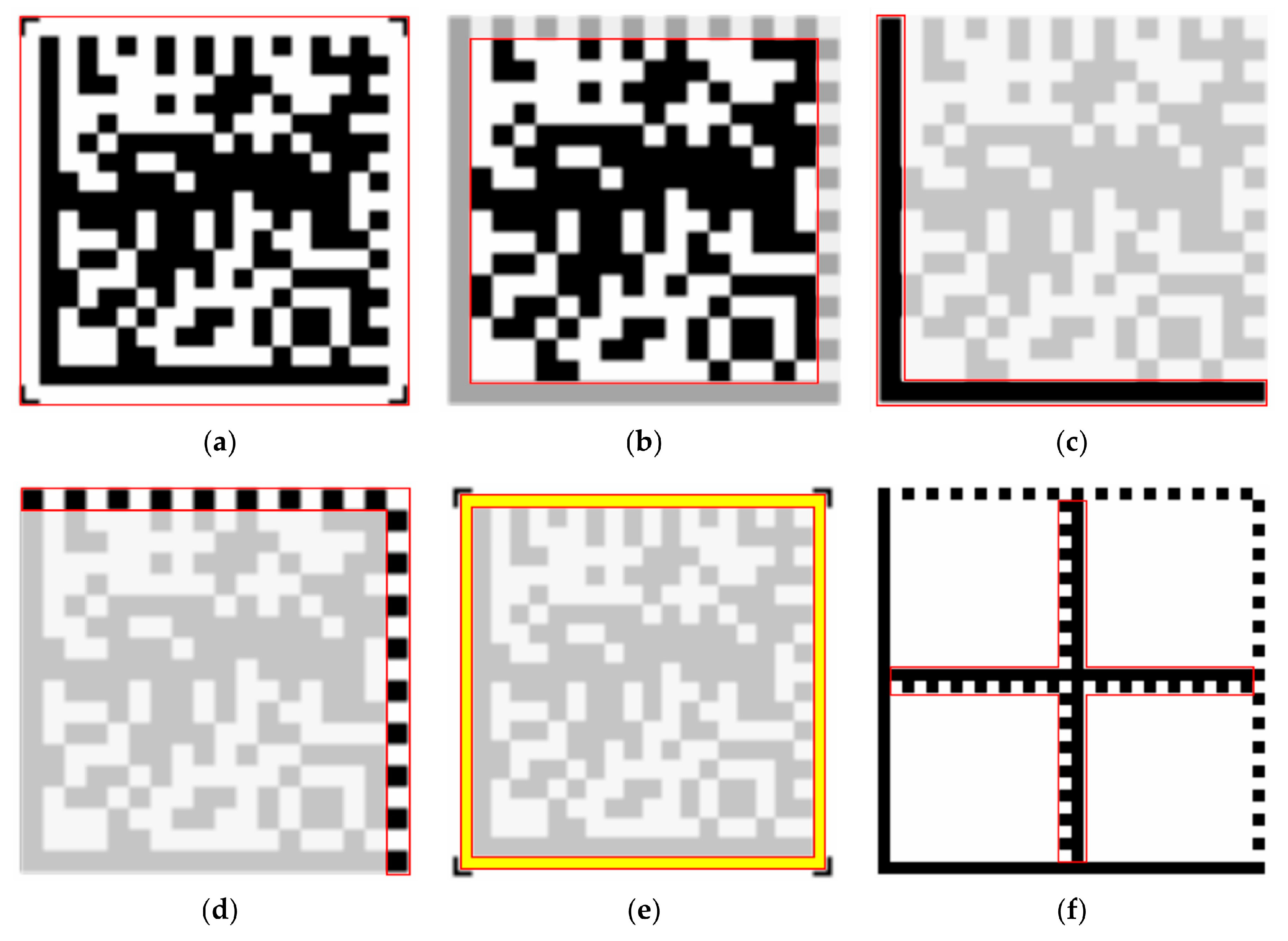
Figure 1. DM code structure in red lines: (a) complete DM code; (b) data regions; (c) finder pattern; (d) finder pattern; (e) quiet zone; (f) alignment pattern.
Electronics 14 02395 g001
Figure 2. Application scenarios: (a) chip; (b) test tube; (c) microbial mass spectrometer target plate.
Electronics 14 02395 g002
Figure 3. The workflow of the adaptive sampling grid division method.
Electronics 14 02395 g003
Figure 4. Grayscale distribution diagram: (a) standard DM code; (b) horizontal grayscale distribution diagram; (c) vertical grayscale distribution diagram.
Electronics 14 02395 g004
Figure 5. Process diagram of horizontal peak detection in Figure 4b.
Electronics 14 02395 g005
Figure 6. Grayscale distribution diagram: (a) DM code in actual scenario; (b) horizontal grayscale distribution diagram; (c) vertical grayscale distribution diagram.
Electronics 14 02395 g006
Figure 7. Process diagram of horizontal peak detection in Figure 6b.
Electronics 14 02395 g007
Figure 8. Histogram of horizontal adjacent peak spacing in Figure 6a.
Electronics 14 02395 g008
Figure 9. Adaptive sampling grid division diagram: (a) adaptive sampling grid division diagram of Figure 4a; (b) adaptive sampling grid division diagram of Figure 6a.
Electronics 14 02395 g009
Figure 10. Grayscale change trend of partial grid.
Electronics 14 02395 g010
Figure 11. A diagram of the grayscale change trend of the 7th grid in the 8th row of the 1st subgraph of Figure 10 after adding abnormal points and repairing them through abnormal point detection.
Electronics 14 02395 g011
Figure 12. Grayscale value predicted by locally weighted linear regression in Figure 11.
Electronics 14 02395 g012
Figure 13. Converting DM code image into data matrix.
Electronics 14 02395 g013
Figure 14. Test images: (a) standard 24 × 24 DM code image; (b) standard 12 × 12 DM code image; (c) DM code label on butterfly specimen; (d) DM code label on plant specimen; (e) DM code etched on caliper; (f) DM code etched on machine part; (g) DM code etched on chip; (h) DM code on bottle; (i) DM code labels on medicine box; (j) DM code labels on medicine box; (k) DM code on microbial mass spectrometer target plate; (l) DM code on microbial mass spectrometer target plate.
Electronics 14 02395 g014
Figure 15. Experimental results of sampling grid division: (a) standard DM code image; (b) standard DM code image; (c) indicates high accuracy; (d) indicates effectiveness; (e) indicates high accuracy; (f) indicates good robustness; (g) indicates high accuracy; (h) indicates good robustness; (i) indicates high accuracy; (j) indicates good robustness; (k) indicates good robustness; (l) indicates good robustness.
Electronics 14 02395 g015
Figure 16. DM code reconstruction diagram of Figure 15: (a) standard 24 × 24 DM code image; (b) standard 12 × 12 DM code image; (c) DM code label on butterfly specimen; (d) DM code label on plant specimen; (e) DM code etched on caliper; (f) DM code etched on machine part; (g) DM code etched on chip; (h) DM code on bottle; (i) DM code labels on medicine box; (j) DM code labels on medicine box; (k) DM code on microbial mass spectrometer target plate; (l) DM code on microbial mass spectrometer target plate.
Electronics 14 02395 g016
Figure 17. Sampling grid division diagram when finder pattern is damaged: (a) standard 24 × 24 DM code image; (b) DM code etched on caliper.
Electronics 14 02395 g017
Figure 18. Line charts of experimental results of Dataset A.
Electronics 14 02395 g018
Figure 19. Line charts of experimental results of Dataset B.
Electronics 14 02395 g019
Figure 20. Samples of DM code images of Dataset A with varying levels of Gaussian noise added: (a) 19%; (b) 51%; (c) 68%.
Electronics 14 02395 g020
Figure 21. Samples of DM code images of Dataset B with varying levels of Gaussian noise added: (a) 6%; (b) 14%; (c) 37%.
Electronics 14 02395 g021
Figure 22. Samples of DM code images of Dataset A with varying levels of spherical distortion added: (a) −15%; (b) −22%; (c) −30%; (d) 15%; (e) 47%; (f) 88%.
Electronics 14 02395 g022
Figure 23. Samples of DM code images of Dataset A with varying levels of spherical distortion added: (a) −17%; (b) −25%; (c) −30%; (d) 23%; (e) 28%; (f) 31%.
Electronics 14 02395 g023
Table 1. The computational complexity of Algorithm 1.
Time ComplexitySpace Complexity
O(x × L × logL × p)O(x × t + p)
Table 2. The computational complexity of Algorithm 2.
Time ComplexitySpace Complexity
O(m × (nlogn + n2))O(m × n)
Table 3. Comparison with libdmtx and zxing of execution time and memory consumption.
DatasetAlgorithmAverage Execution Time(s)Average Memory Consumption (KB)
Alibdmtx0.00235.600
zxing0.4355.000
this paper5.133244.800
Blibdmtx0.00460.364
zxing0.3566.909
this paper14.971329.454
Disclaimer/Publisher’s Note: The statements, opinions and data contained in all publications are solely those of the individual author(s) and contributor(s) and not of MDPI and/or the editor(s). MDPI and/or the editor(s) disclaim responsibility for any injury to people or property resulting from any ideas, methods, instructions or products referred to in the content.