Multi-Objective Trajectory Planning for Robotic Arms Based on MOPO Algorithm

Abstract

This research describes a multi-objective trajectory planning method for robotic arms based on time, energy, and impact. The quintic Non-Uniform Rational B-Spline (NURBS) curve was employed to interpolate the trajectory in joint space. The quintic NURBS interpolation curve can make the trajectory become constrained within the kinematic limits of velocity, acceleration, and jerk while also satisfying the continuity of jerk. Then, based on the Parrot Optimization (PO) algorithm, through improvements to reduce algorithmic randomness and the introduction of appropriate multi-objective strategies, the algorithm was extended to the Multi-Objective Parrot Optimization (MOPO) algorithm, which better balances global search and local convergence, thereby more effectively solving multi-objective optimization problems and reducing the impact on optimization results. Subsequently, by integrating interpolation curves, the multi-objective optimization of joint trajectories could be performed under robotic kinematic constraints based on time–energy-jerk criteria. The obtained Pareto optimal front can provide decision-makers in industrial robotic arm applications with flexible options among non-dominated solutions.

1. Introduction

Trajectory planning is fundamental to robotic applications, as it ensures the successful execution of assigned tasks and governs the efficiency and accuracy of task completion. The rapid development of robotic arm technology in recent years has led to progressively stricter demands in their operational environments. Consequently, the performance demands on robotic arms have also grown, and the performance requirements for robotic arms vary under different working conditions. Trajectory optimization for robotic arms has always been the goal pursued by researchers.

Trajectory planning investigates the time-dependent relationship of a robot’s pose during motion, aiming to describe the state of joint parameters at specific time points. Currently, there exist numerous trajectory planning methods for robotic arm joint space, which can generally be described through two distinct phases: The first phase involves joint trajectory interpolation, where joint paths are processed through interpolation techniques. Common interpolation methods include polynomial interpolation, B-spline curves, NURBS, and so on. The second phase focuses on trajectory optimization. Following on from the interpolation process, optimization algorithms are employed to refine time nodes, ensuring trajectory smoothness and enhancing the robotic arm’s operational efficiency. Through these two phases of processing, precise and efficient robotic arm trajectory planning can be achieved.

The joint trajectory interpolation of robotic arms involves constructing joint trajectories using different interpolation curves based on specific task requirements and the posing of information at the start and end points. Regarding this, scholars worldwide have conducted extensive discussions. For instance, Wang et al. [1] established a 3-5-3 polynomial interpolation function as the foundation for trajectory planning and achieved the time-optimal optimization of robotic arm joint trajectories by incorporating an improved cuckoo search algorithm. Dinçer et al. [2] integrated cubic polynomials with Bézier curves using quadratic Bernstein basis functions to develop a new hybrid polynomial. The experimental results demonstrated that this composite polynomial could achieve smoother motion trajectories while significantly reducing mechanical vibrations. Boryga [3] proposed a smooth trajectory generation approach based on high-degree polynomial functions. The research formulated acceleration polynomials and determined exact analytical relationships for time and coefficients while satisfying constraints. Liu et al. [4] employed cubic B-splines for trajectory interpolation and the integrated particle swarm optimization algorithm to optimize motion time. The experimental results demonstrated that this approach provides an optimal trajectory solution for robotic arm joint space applications. Li et al. [5] proposed a smooth trajectory planning method that decomposes the path into two orthogonal coordinate axes and subsequently employs quintic B-spline curves to generate motion profiles. This approach achieves continuous and stable joint trajectories while significantly reducing end-effector residual vibrations. Lan et al. [6] employed seventh-degree B-spline curves to generate smooth joint motion profiles, ensuring continuity in collaborative robot joint curves. Fang et al. [7] proposed an S-curve-based trajectory planning method that constructs joint trajectories using piecewise S-functions. This approach achieves more efficient and computationally simpler trajectory planning compared to conventional polynomial methods while allowing adjustable trade-offs between efficiency and smoothness through limit value modulation. Wang [8] developed an innovative NURBS-based contour control strategy for robotic systems. This method utilizes contour errors as a key performance indicator and proposes a tangent-approximation contour error estimation technique, significantly enhancing precision in contour tracking applications.

Trajectory optimization can be classified into single-objective and multi-objective methods. The former concentrates on optimizing one particular performance criterion while neglecting other factors, whereas the latter simultaneously handles multiple competing objectives. Multi-objective optimization typically involves obtaining Pareto optimal solutions, from which the most suitable compromise solution is chosen based on practical application requirements and constraints. Han et al. [9] proposed an enhanced Particle Swarm Optimization (PSO) algorithm that effectively addresses the local optima entrapment problem inherent in conventional approaches. The improved algorithm achieves superior optimization outcomes through better equilibrium between exploration and exploitation capabilities. Du et al. [10] proposed a novel locally chaotic particle swarm optimization algorithm that effectively resolves the premature convergence issue inherent in conventional algorithms. Zhang et al. [11] employed hybrid inverse kinematics to compute critical sequence points for joint trajectories, subsequently proposing an adaptive cuckoo search algorithm with enhanced convergence properties. This methodology successfully generated smooth, time-optimal trajectories while satisfying dynamic constraints. Zhang et al. [12] partitioned the joint space of the robotic arm and subsequently proposed an enhanced sparrow search algorithm. The algorithm enhanced both convergence speed and search capability through the integration of chaotic mapping and adaptive step-size adjustment, ultimately generating smooth operational trajectories. Xu et al. [13] obtained a trajectory with smooth angular velocity and no acceleration jump by combining the multi-population search strategy of the Harris Hawks algorithm with the quintic polynomial interpolation trajectory. Li et al. [14] proposed a stability-constrained trajectory planning method that incorporates an enhanced version of Non-Dominated Sorting Genetic Algorithm-II (NSGA-II) to simultaneously optimize both execution time and energy consumption for robotic arm trajectories, thereby improving motion stability. Shi et al. [15] applied multi-objective optimization to address trajectory planning. They considered both kinematic and dynamic constraints. The researchers developed a normalized weighted objective function. This function helped select optimal solutions from the Pareto front. This method successfully generated high-order continuous optimal trajectories. Yang et al. [16] integrated multiple improvement strategies into the Whale Optimization Algorithm (WOA). The resulting Multi-Strategy Whale Optimization Algorithm (MSWOA) showed substantially better search performance. This algorithm proves particularly effective for global optimization challenges. Liu et al. [17] developed an improved multiverse algorithm by enhancing the wormhole probability curve, adaptively adjusting parameters, and incorporating population mutation fusion. The proposed algorithm improves convergence speed and global search capability, thereby enhancing the comprehensive performance of robotic arms. Liu et al. [18] proposed an improved multi-objective grasshopper optimization algorithm that effectively addresses multi-objective optimization in orthogonal robots, significantly mitigating operational unevenness issues. Xu et al. [19] developed a multi-objective trajectory planning approach for spraying robots. This method combines the “7-5-7” hybrid interpolation technique with the hybrid multi-objective NSGA-II algorithm. Tests show that optimized paths achieve faster operation, less energy use, and have minimized mechanical impact.

In summary, numerous scholars have conducted in-depth research on interpolation and optimization methods for robotic trajectory planning. These studies mainly use interpolation methods such as polynomials, B-splines, and NURBS to construct joint trajectories and then employ optimization algorithms to perform trade-off optimization among multiple objectives, including time, energy consumption, and jerk. However, due to the inherent randomness of optimization algorithms, they often face issues during optimization, such as an insufficient global search capability leading to local optima and inadequate local convergence. How to better balance the relationship between global search and local convergence to reduce any impact on the optimization results remains a key research direction in the field of robotic trajectory planning.

This research proposes a multi-objective trajectory planning method for robotic arms based on the MOPO algorithm to address three key performance metrics during operation: time, energy, and impact. This method utilizes quintic NURBS to construct joint trajectories for the robotic arm, ensuring the continuity and smoothness of the motion paths. Subsequently, the joint trajectories are optimized using an improved MOPO algorithm, which incorporates enhanced parrot optimization techniques and introduces multi-objective strategies. Finally, experimental results verify the performance advantages of the algorithm and demonstrate the effectiveness of the proposed method for solving multi-objective robotic trajectory planning problems.

The preceding sections are arranged as follows: Section 2 presents the trajectory planning problem and selects quintic NURBS curves to construct joint trajectories. Section 3 elaborates on the enhanced parrot optimization algorithm and presents the developed MOPO algorithm through the incorporation of multi-objective strategies. Section 4 presents the analytical results of algorithmic performance comparisons along with comparative evaluations of the optimization outcomes obtained through multi-objective trajectory planning for the robotic arm. Finally, Section 5 outlines the main conclusions.

2. Trajectory Planning

2.1. Construction of Joint Trajectory Based on Quintic NURBS

The interpolation methods currently applied to robotic arm joint trajectories primarily include polynomial interpolation, B-spline curves, and NURBS. Specifically, polynomial interpolation offers computational simplicity and guarantees trajectory continuity but may generate significant oscillations between interpolation points, resulting in trajectory instability. Furthermore, when dealing with complex trajectory shapes, polynomial interpolation often fails to achieve satisfactory fitting performance and maintain stability, thus limiting its simplicity to simple, continuous trajectories only. B-spline curves are composed of multiple control points and basis functions, which can more flexibly describe complex trajectories and effectively avoid oscillations and sudden velocity changes in robotic arm trajectories. However, B-spline curves typically do not pass through all control points and are only influenced by them, making them unsuitable for tasks requiring precise passage through specified points. In contrast, NURBS improves upon B-spline curves by introducing weight adjustments that provide more flexible curve shape modifications, enabling the curve to pass through specific points without affecting the overall control point arrangement. This NURBS interpolation guarantees that the curve passes through all trajectory points, thereby providing a more precise description of robotic arm joint trajectories and making it better suited to high-performance robotic arm trajectory planning tasks. Furthermore, to ensure smooth robotic arm motion while considering computational complexity, this research adopts quintic NURBS for interpolating the robotic arm’s joint trajectories.

The quintic NURBS was first derived to construct the joint trajectory curve. For robotic arms, the joint velocity, acceleration, and jerk, respectively, at the time node $u\in [u_i,u_{i+1}]$ can be expressed as follows:

$$P^r\left(u\right)=\sum _{j=i-k+r}^i{d}_j^r{N}_{j,k-r}(u)$$

(1)

$$d_j^i=\left\{\begin{array}{c}{d}_j\\ (k+1-l){\displaystyle \frac{d_j^{l-1}-d_{j-1}^{l-1}}{u_{j+k+1-l}-u_j}}\end{array}\right.$$

(2)

where r = 1, 2, 3.

In Equation (1), $d_j^r$ represents the control vertex; $P(u)$ is the joint position at time $u$; and $N_{j,k-r}(u)$ is the normalized k-r th degree B-spline basis function for the j th segment, which can be recursively computed via the De Boor–Cox formula:

$$\left\{\begin{array}{c}{N}_{i,0}(u)=\left\{\begin{array}{cc}0,& u_i\le u<u_{i+1}\\ 1,& \mathit{else}\end{array}\right.\\ N_{j,k-r}(u)={\displaystyle \frac{(u-u_j)N_{j,k-r-1}(u)}{u_{j+k-r}-u_j}}+{\displaystyle \frac{(u_{j+k-r+1}-u)N_{j+1,k-r+1}(u)}{u_{j+k-r+1}-u_{j+1}}}\end{array}\right.$$

(3)

The knot vector $u=[u_0,u_1,\dots ,u_{n+2k}]$ is then normalized to satisfy the following requirements:

$$u_0=u_1=\dots {=u}_k=0$$

(4)

$$u_{n+k}=u_{n+k+1}=\dots {=u}_{n+2k}=1$$

(5)

$$u_i=u_{i-1}+{\displaystyle \frac{\left|∆t_{i-1-k}\right|}{{\sum }_{j=0}^{n-1}\left|∆t_j\right|}} i=k+1,\dots ,n+k-1$$

(6)

After determining the time nodes, the corresponding constraint equation for the time-position sequence can be obtained:

$$\mathrm{P}\left(u_{i+k}\right)=\sum _{j=i}^{i+k}{d}_j{N}_{j,k}\left(u_{i+k}\right)=P_i$$

(7)

where i = 1, 2, …, n, $d_j$ represents the control vertex vector, j = 0, 1, …, n + k − 1.

Given the time-position sequence $S=(p_i,t_i)$ and the total motion duration $t_{\mathit{sum}}={\sum }_{i=0}^n{t}_i$, the following relation was derived from Equation (6):

$$u_i=u_{i-1}+{\displaystyle \frac{\left|∆t_{i-6}\right|}{{\sum }_{j=0}^{n-1}\left|∆t_j\right|}}\hspace{1em}i=6,\dots ,n+4$$

(8)

From the analysis of the equation, it is evident that the number of control points was n + k. To fully determine the B-spline curve, an additional k − 1 equation was required. Given the known initial/final velocities and accelerations of the joint motion, and to ensure the smoothness of motion, the initial/final velocities and accelerations for all joints could be set to zero. This introduced four additional boundary conditions as follows:

$$\left\{\begin{array}{c}{w}_0=P^{\prime }\left(u_5\right)=0, w_f=P^{\prime }\left(u_{n+5}\right)=0\\ a_0=P^{″}\left(u_5\right)=0, a_f=P^{″}\left(u_{n+5}\right)=0\end{array}\right.$$

(9)

In summary, the inverse calculation equations for determining the control points can be expressed as follows:

$$\left\{\begin{array}{c}{A}_{n}d=P\\ d=[d_0,d_1,\dots ,d_n,d_{n+1},\dots ,d_{n+4}]\\ P=[P_0,P_1,\dots ,P_n,w_0,w_f,a_0,a_f]\end{array}\right.$$

(10)

where $A_n\in R^{(n\times 5)\times (n\times 5)}$ is the coefficient matrix.

The control vertex vector can be obtained from Equation (10) as follows:

$$d=A_n^{-1}P$$

(11)

By utilizing the control point vector d and time nodes, u, the continuous joint trajectory sequence can be computed. Subsequently, the velocity, acceleration, and jerk profiles of the joint motion can be derived from Equation (1).

2.2. Establishment of Objective Function and Kinematic Constraints

In the optimization of robotic arms joint trajectories, it is essential to first identify the optimization objectives and formulate corresponding objective functions. Furthermore, due to the inherent kinematic constraints of robotic arms, constraint conditions must be defined to construct a multi-objective trajectory planning mathematical model. The objective function is initially defined as follows:

$$\left\{\begin{array}{c}{S}_1=T={\displaystyle \sum _{i=0}^{n-1}}(t_{i+1}-t_i)\\ S_2={\displaystyle \sum _{\mathit{m}=1}^{\mathit{M}}}\sqrt{{\displaystyle \frac{1}{T}}{\int }_0^T{a}_i^2\mathit{dt}}\\ S_3={\displaystyle \sum _{\mathit{m}=1}^{\mathit{M}}}\sqrt{{\displaystyle \frac{1}{T}}{\int }_0^T{j}_i^2\mathit{dt}}\end{array}\right.$$

(12)

where $S_1$ represents the total execution time, which reflects the duration required for the robotic arm to complete the task. A shorter execution time typically indicates higher operational efficiency. $S_2$ denotes the mean joint acceleration, directly correlated with energy consumption, where higher acceleration generally leads to increased energy expenditure. $S_3$ corresponds to the mean joint jerk, characterizing the rate of change in joint angular acceleration, which is directly associated with mechanical shock during robotic arm motion.

Additionally, the robotic arm is subject to inherent kinematic constraints, which primarily include the following:

$$\left\{\begin{array}{c}{g}_1\left(t\right)=\left|{\mathit{q}}_i(t)\right|-{\mathit{Q}}_{\mathit{jmax}} \le 0\\ g_2\left(t\right)=\left|{\mathit{v}}_i(t)\right|-{\mathit{V}}_{\mathit{jmax}} \le 0\\ g_3\left(t\right)=\left|a_i(t)\right|-A_{\mathit{jmax}} \le 0\end{array}\right.$$

(13)

where ${\mathit{Q}}_{\mathit{jmax}}$ represents the joint angle limits, and ${\mathit{q}}_i(t)$ denotes the joint angles; ${\mathit{V}}_{\mathit{jmax}}$ indicates the joint velocity limits, while ${\mathit{v}}_i(t)$ stands for the joint velocities; and $A_{\mathit{jmax}}$ specifies the joint acceleration limits, with $a_i(t)$ representing the joint accelerations.

For the multi-objective trajectory planning problem of robotic arms, the optimization variables are the time intervals $∆t_i=t_{i+1}-t_i$ between consecutive positional waypoints. During the optimization process, interpolation curves are employed to generate joint trajectories based on the optimized time variables at each iteration, thereby enabling the computation of each objective function value specified in Equation (12). Concurrently, the algorithm checks whether the interpolated joint angles, velocities, and accelerations exceed the kinematic constraints of the robotic arm, i.e., whether the constraint conditions in Equation (13) are satisfied. When constraint violations occur, the corresponding solution is penalized by assigning an extremely large value to all associated objective functions, thereby discarding this infeasible solution in subsequent iterations and ensuring compliance with the robotic arm’s kinematic constraints.

3. Multi-Objective Parrot Optimization Algorithm

3.1. Parrot Optimization Algorithm

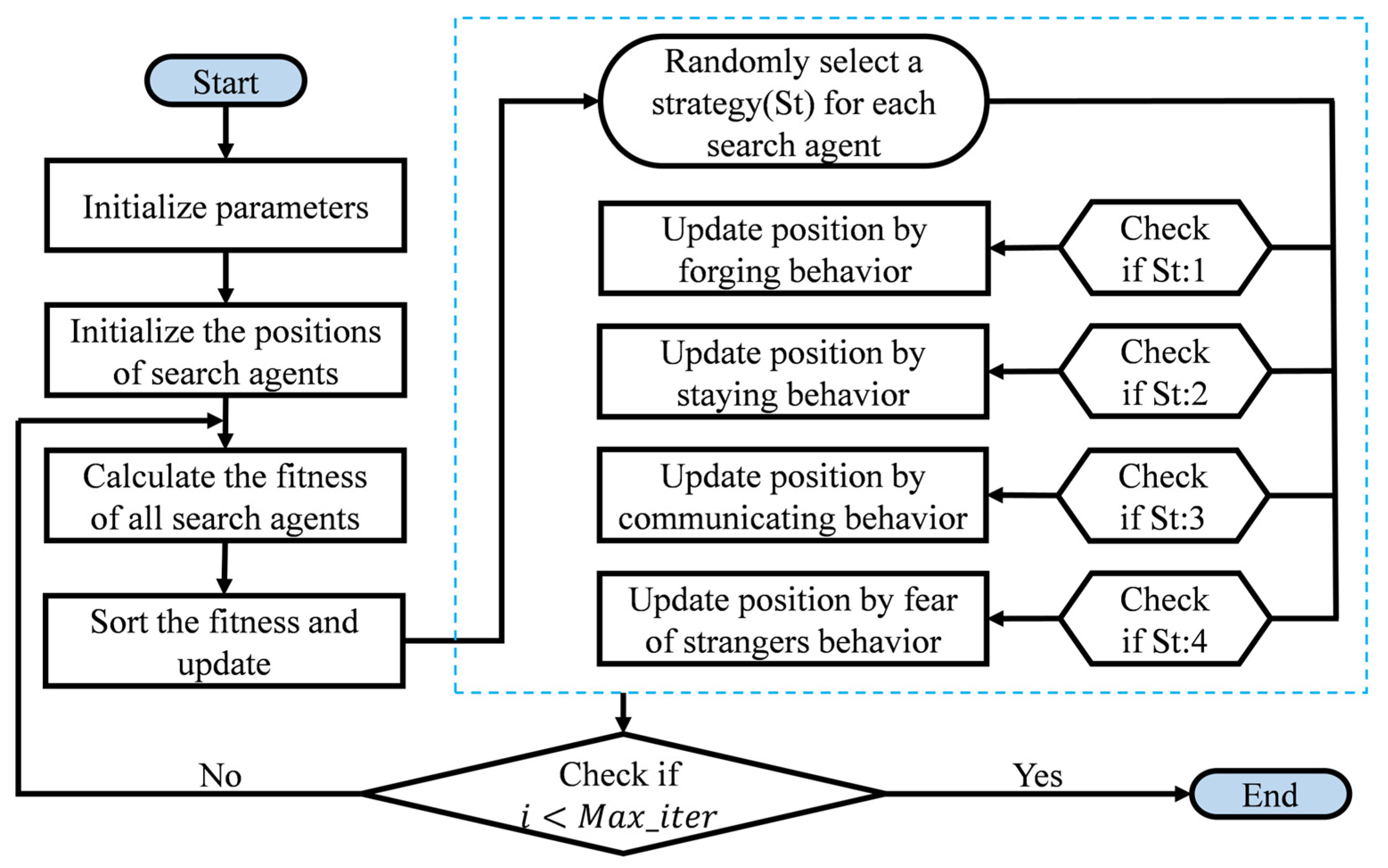
PO is an efficient metaheuristic algorithm inspired by four key behaviors observed in parrot populations: foraging, staying, communicating, and stranger avoidance [20]. These behaviors are mathematically encapsulated through four corresponding computational models in the algorithm:

$${\mathit{X}}_i^{t+1}=({\mathit{X}}_i^t-{\mathit{X}}_{\mathit{best}})\cdot \mathit{Levy}(\mathit{dim})+\mathit{rand}(0,1)\cdot (1-{\displaystyle \frac{t}{{\mathit{Max}}_{\mathit{iter}}}}{)}^{{\displaystyle \frac{2t}{{\mathit{Max}}_{\mathit{iter}}}}}\cdot {\mathit{X}}_{\mathit{mean}}^t$$

(14)

$${\mathit{X}}_i^{t+1}={\mathit{X}}_i^t+{\mathit{X}}_{\mathit{best}}\cdot \mathit{Levy}\left(\mathit{dim}\right)+\mathit{rand}\left(0,1\right)\cdot \mathit{ones}\left(1,\mathit{dim}\right)$$

(15)

$${\mathit{X}}_i^{t+1}=\left\{\begin{array}{c}0.2\cdot rand\left(0,1\right)\cdot \left(1-{\displaystyle \frac{t}{{\mathit{Max}}_{\mathit{iter}}}}\right)\cdot \left({\mathit{X}}_i^t-{\mathit{X}}_{\mathit{mean}}^t\right), P \le 0.5\\ 0.2\cdot rand(0,1)\cdot \mathit{e}\mathit{x}p\left(-{\displaystyle \frac{t}{\mathit{rand}\left(0,1\right)\cdot {\mathit{Max}}_{\mathit{iter}}}}\right), P > 0.5\end{array}\right.$$

(16)

$$\begin{gathered} {\mathit{X}}_i^{t+1}={\mathit{X}}_i^t+\mathit{rand}\left(0,1\right)\cdot \cos \left(0.5\pi \cdot {\displaystyle \frac{t}{{\mathit{Max}}_{\mathit{iter}}}}\right)\cdot \left({\mathit{X}}_{\mathit{best}}-{\mathit{X}}_i^t\right) \\ -\cos \left(\mathit{rand}\left(0,1\right)\cdot \pi \right)\cdot {\left({\displaystyle \frac{t}{{\mathit{Max}}_{\mathit{iter}}}}\right)}^{{\displaystyle \frac{2}{{\mathit{Max}}_{\mathit{iter}}}}}\cdot \left({\mathit{X}}_i^t-{\mathit{X}}_{\mathit{best}}\right) \end{gathered}$$

(17)

Unlike traditional metaheuristic algorithms, during each iteration, every individual in the PO population randomly exhibits one of these four behaviors—that is, each individual randomly selects one strategy to update its search process rather than following a fixed update pattern. This approach offers a more biologically faithful representation of behavioral stochasticity observed in parrots while substantially improving population diversity. The randomized architecture of PO distinguishes it from conventional algorithms, effectively mitigating local optima entrapment risks while preserving solution quality.

In the PO algorithm, an initial population of random solutions is first generated. These candidate solutions are then iteratively updated using the current best solution and predefined update rules to search for the global optimum. During optimization, each individual continuously adjusts its position dynamically until specified termination criteria are met. Figure 1 shows the complete flowchart of the PO algorithm.

3.2. Multi-Objective Parrot Optimization Algorithm

In the PO algorithm, the random selection of an update strategy during each iteration introduces a high degree of randomness. This may lead to insufficient exploration depth or susceptibility to local optima. To address these issues, this research introduces several modifications to the original algorithm.

In the original algorithm, the selection of one of the four strategies during each iteration is determined by a random number, resulting in a high degree of randomness. To address this, this research introduces the parameter $i/{\mathit{Max}}_{\mathit{iter}}$, representing the ratio of the current iteration count to the total iteration count. During each iteration, the ratio $i/{\mathit{Max}}_{\mathit{iter}}$ is compared with a constant, a, to assess the progress of the algorithm and adjust the probabilities of selecting each strategy. Among the four update strategy formulations in the PO algorithm, Equations (14) and (16) correspond to the algorithm’s exploration (breadth search), while Equations (15) and (17) are responsible for exploitation (depth search). Therefore, in the improved algorithm, by judging the iterative process of the algorithm and adjusting the probability of selecting each strategy dynamically, it is ensured that there is a greater probability of selecting the breadth search strategy formula in the early stages of the algorithm, so as to effectively prevent premature convergence to local optima. Conversely, in the later stages, the probability of selecting exploitation strategies is increased to enhance the depth-searching capability, thereby improving the accuracy of convergence towards the optimal solution.

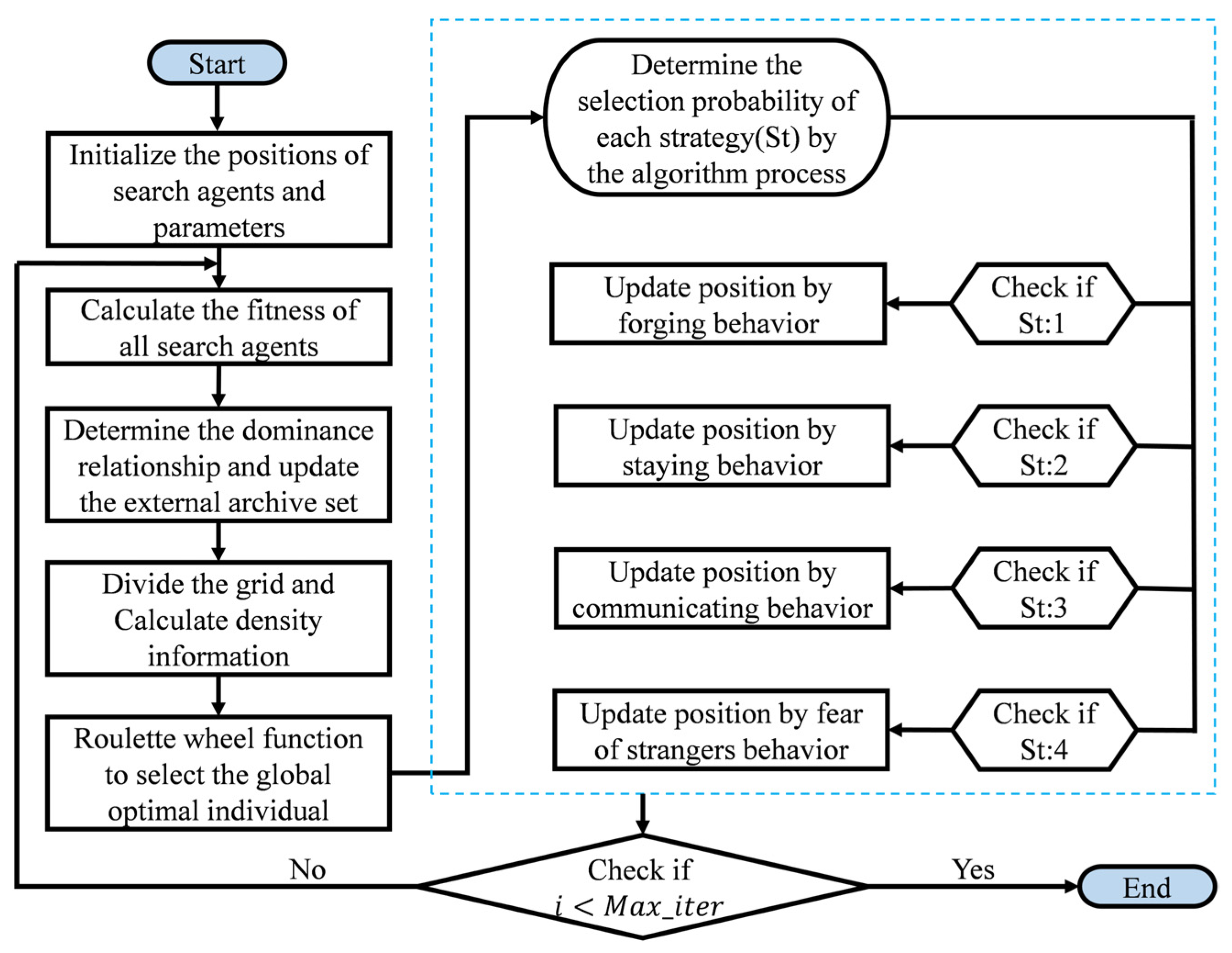
Currently, solving multi-objective optimization problems using similar optimization algorithms generally follows two approaches: One is to deal with multiple objective function problems through weighted summation, gray correlation analysis, the analytic hierarchy process, and other methods, transform multi-objective problems into a single-objective optimization problem, and then apply single-objective optimization algorithm for optimization. The second is to establish mathematical functions that can evaluate and select the most favorable solutions for individuals and the overall population during the iterative process. A multi-objective optimization algorithm is then employed to iteratively generate an optimal Pare-to solution set, from which the most suitable solutions are selected according to task requirements. Multi-objective optimization refers to solving two or more mixed objective functions under certain constraints. In multi-objective trajectory optimization problems, it is often challenging to determine appropriate weights for the various objective functions, and these objectives may sometimes come into conflict with one another. As a result, traditional single-objective optimization methods are often inadequate for solving such problems. This research adopts the second approach. On the basis of improving the PO algorithm, strategies such as dominance relationships, external archive sets, grid partitioning, and roulette wheel selection are introduced to adapt the algorithm for multi-objective optimization. The resulting MOPO algorithm is designed to comprehensively solve problems involving multiple objective functions.

First, the dominance relationship is defined as follows: A solution p is said to dominate solution q if and only if both of the following conditions are satisfied: (1) for all objective functions, p is not worse than q, i.e., $f_k\left(p\right)\le f_k\left(\mathit{q}\right)$, (k = 1, 2, …, r); (2) there exists at least one objective function where p is strictly better than q, i.e., $\exists l\in \left\{1,2,\dots ,r\right\}$ such that $f_l\left(p\right)<f_l\left(\mathit{q}\right)$. In addition, in single-objective optimization, where only one objective function exists, selecting the global best individual is straightforward by comparing the value of the objective function. However, in multi-objective optimization, where multiple objective functions are typically involved, the direct comparison of individual objective function values is not applicable. In the MOPO proposed in this research, the global best individual is selected as follows: First, an external archive set $\psi$ is defined to store non-dominated individuals discovered during the search process. During each iteration, grids are generated and divided based on all individuals in the external archive. The grid boundaries are determined by the maximum and minimum values. The number of individuals in each grid is then used as a fitness value for roulette wheel selection. The fitness values are inverted, so smaller fitness values have a higher probability of being selected. This approach ensures diversity among the solutions. Once a grid is selected, a random individual within that grid is chosen as the global best individual for updating the algorithm in the current iteration.

The main difference between MOPO and the original single-objective algorithm during iteration lies in the following processes: initializing the state information of n particles in the population and setting the maximum size of the external archive set to N; dividing the entire population into a dominant set W and a non-dominant set Q based on fitness dominance relationships, and placing the particles in Q into the external archive set Ψ; during updates, the dominant set, W, is first updated, calculating the fitness of the new dominant set W, and then processing the dominance relationships with the non-dominant set Q to update W and Q. A new solution can only be incorporated into the external archive set if it is non-dominated with respect to all existing solutions within the archive. Furthermore, any archived solution that becomes dominated by newly introduced solutions during this process will be systematically removed. The population is iteratively updated, and when the termination condition is met, the population optimization is completed, resulting in the Pareto solution set, which represents a set of optimal solutions.

At this point, the MOPO algorithm is obtained. The flowchart of the algorithm is illustrated in Figure 2.

The pseudocode of the MOPO algorithm (Algorithm 1) is presented below, where Pop represents the population, Obj_fun denotes the function for calculating objective function values, Const_fun indicates the function for evaluating constraint conditions, Dominate_fun represents the function for determining dominance relationships, Grid_fun and Roulette_fun represent the functions used to divide the grid and the function of selecting the global best solution, respectively; finally, St_fun represents the function of selecting the update strategy.

Algorithm 1 MOPO Algorithm

1:  Initialize the MOPO parameters 2:  Initialize the Pop’ positions randomly 3:  Obj_fun(Pop) and Const_fun(Pop) 4:  Initialize individual best solution Pbest 5:  Archive ← Dominate_fun(Pop) $$\begin{gathered} 6: \mathbf{For} i=1: {\mathit{Max}}_{\mathit{iter}} \mathbf{do} \\ 7: \mathbf{For} j=1: N \mathbf{do} \\ 8: G_{\mathit{best}} \leftarrow \mathrm{Grid}\_\mathrm{fun}(\mathrm{Archive}) \mathrm{and} \mathrm{Roulette}\_\mathrm{fun}(\mathrm{Archive}) \\ 9: \mathrm{St}\_\mathrm{fun}(i) \\ 10: \mathbf{If} \mathrm{St}==1 \mathbf{Then} \\ 11: \mathrm{Update} \mathrm{Pop}’ \mathrm{positions} \mathrm{by} \mathrm{Equation} (14) \\ 12: \mathbf{Elseif} \mathrm{St}==2 \mathbf{Then} \\ 13: \mathrm{Update} \mathrm{Pop}’ \mathrm{positions} \mathrm{by} \mathrm{Equation} (15) \\ 14: \mathbf{Elseif} \mathrm{St}==3 \mathbf{Then} \\ 15: \mathrm{Update} \mathrm{Pop}’ \mathrm{positions} \mathrm{by} \mathrm{Equation} (16) \\ 16: \mathbf{Elseif} \mathrm{St}==4 \mathbf{Then} \\ 17: \mathrm{Update} \mathrm{Pop}’ \mathrm{positions} \mathrm{by} \mathrm{Equation} (17) \\ 18: \mathbf{End} \\ 19: \mathrm{Obj}\_\mathrm{fun}(\mathrm{Pop}) \mathrm{and} \mathrm{Const}\_\mathrm{fun}(\mathrm{Pop}) \\ 20: \mathrm{Update} P_{\mathit{best}} \leftarrow \mathrm{Dominate}\_\mathrm{fun}(P_{\mathit{best}},\mathrm{Pop}) \end{gathered}$$ 21:        Update Archive ← Dominate_fun (Archive, Pop) 22:      End 23:  End

4. Simulation Verification and Analysis

After completing the derivation of the MOPO algorithm, two experimental subsections are designed for comparative verification to ensure the proposed method can be effectively applied to multi-objective trajectory planning for robotic arms. First, the obtained MOPO algorithm is validated using standard multi-objective test functions, with comparative analysis conducted to examine its effectiveness in solving multi-objective optimization problems and its performance advantages. Subsequently, by integrating interpolation curves, the multi-objective optimization of joint trajectories is performed under robotic kinematic constraints based on time–energy–jerk criteria, verifying the effectiveness of the proposed method for solving robotic multi-objective trajectory planning problems.

4.1. Testing Environment

The simulation was conducted on a system equipped with a 12th Gen Intel^® Core™ i7-12700 20-core processor and 16 GB of RAM (Lenovo, Tianjin, China). Computational experiments were conducted on a Windows 11 operating system using MATLAB R2020a as the simulation platform.

4.2. Performance Verification of MOPO Algorithm

In multi-objective optimization problems, evaluation metrics can generally be categorized into convergence metrics and diversity metrics based on the different emphases of an assessment, which measure the convergence and distribution characteristics of the obtained solution sets, respectively. Among them, the Generational Distance (GD) [21] is one of the most classical convergence metrics, the value of which represents the distance between the non-dominated solution set obtained by the algorithm and the ideal reference Pareto front. A smaller GD value indicates the better convergence of the solution set, meaning that the algorithm exhibits stronger convergence capability, thereby yielding solutions closer to the true Pareto front. This metric reflects the algorithm’s local convergence ability and is defined as follows:

$$\mathit{GD}={\displaystyle \frac{\sqrt{{\sum }_{i=1}^n{d}_i^2}}{n}}$$

(18)

where n represents the number of non-dominated solutions obtained by the algorithm, and d_i denotes the Euclidean distance between the solution x_i and Pareto front.

Among diversity metrics, the Spacing (SP) [22] metric serves as a representative indicator. Its value is derived from the standard deviation of the minimum distances between each solution and its nearest neighboring solution in the obtained non-dominated set. A smaller SP value indicates the more uniform spatial distribution of solutions within the solution set, demonstrating the algorithm’s stronger exploration capability, yielding a better diversity for non-dominated solutions. This metric quantitatively evaluates the distribution characteristics of the solution set, thereby reflecting the algorithm’s global search performance, formally defined as follows:

$$\mathit{SP}=\sqrt{{\displaystyle \frac{1}{n-1}}{\sum }_{i=1}^n{(d-{\mathit{do}}_i)}^2}$$

(19)

where do_i represents the Euclidean distance between solution x_i and its nearest neighboring solution in the obtained non-dominated set, and d denotes the arithmetic mean of all do_i values.

When evaluating the algorithm’s performance using the aforementioned metrics, the true Pareto front of the optimization problem must be precisely defined. The ZDT test functions serve as classical benchmark problems in multi-objective optimization, featuring well-defined Pareto fronts and distinct optimization characteristics that enable an accurate and objective performance assessment. Among them, the Pareto front of the ZDT1 function is continuous and convex; the Pareto front of the ZDT2 function is continuous and concave; and the Pareto front of the ZDT3 function is discrete and non-continuous. These three functions cover optimization problems with different characteristics, such as convexity, concavity, and discreteness, which can more comprehensively evaluate algorithm performance and ensure the completeness of the algorithm’s evaluation. Therefore, the standard test functions ZDT1, ZDT2, and ZDT3 were selected to validate the effectiveness of the MOPO algorithm in solving multi-objective optimization problems, with the representative multi-objective optimization algorithms NSGA-II and MOPSO being chosen as control groups for comparative performance analysis to verify the performance advantages of the proposed MOPO algorithm.

To ensure the fairness and objectivity of the experiments, uniform parameter configurations were set for all algorithms: a population size of 200, an external archive size of 200, and a maximum iteration count of 200. The optimization results of each algorithm on the standard test functions ZDT1, ZDT2, and ZDT3, represented by the obtained Pareto solution sets, are shown in Figure 3, Figure 4, and Figure 5, respectively.

To ensure the reliability of the experimental results, all three algorithms were independently executed 50 times for each standard test function. The average values of both GD and SP evaluation metrics were then calculated, with the detailed results presented in

Table 1. Values of evaluation metrics for each algorithm.

Algorithm	ZDT1		ZDT2		ZDT3
	GD	SP	GD	SP	GD	SP
NSGA-II	2.51 × 10−4	4.93 × 10−3	2.92 × 10−4	3.76 × 10−3	1.08 × 10−3	6.13 × 10−3
MOPSO	2.06 × 10−4	3.74 × 10−3	2.63 × 10−4	4.59 × 10−3	3.59 × 10−4	4.21 × 10−3
MOPO	1.83 × 10−4	1.98 × 10−3	2.14 × 10−4	2.61 × 10−3	2.89 × 10−4	3.17 × 10−3

.

A comprehensive analysis of Figure 3, Figure 4 and Figure 5 shows that to solve these three standard test functions, while both NSGA-II and MOPSO algorithms can converge to the true Pareto front, their solution sets exhibit uneven and discontinuous distributions with some missing solutions. This indicates that these algorithms are prone to the problem of falling to a local optimum due to an insufficient global search ability in the optimization process. In contrast, the Pareto-optimal solution set obtained by the MOPO algorithm demonstrates a more accurate and uniform continuous coverage of the true Pareto front of the test functions, indicating a superior balance between global exploration and local exploitation. Further analysis of the data in Table 1 shows that the MOPO algorithm achieves lower average values for both GD and SP metrics compared to the other two algorithms, indicating better convergence and diversity for the optimal solution set. This more precisely and intuitively reflects its stronger global search capability and local convergence performance, further demonstrating the effectiveness and performance advantages of the proposed MOPO algorithm in solving multi-objective optimization problems.

4.3. Validation of Multi-Objective Trajectory Planning for Robotic Arms

This section adopts the UR5 6-DOF serial robotic arm as a case study. The planned task-space trajectory is transformed into joint-space motion paths through inverse kinematics, yielding the corresponding joint trajectory curves. The characteristic sampling of these joint-space paths generates the discrete path sequence, as presented in

Table 2. Data for trajectory sampling sequence points.

Point	Position (rad)
	Joint 1	Joint 2	Joint 3	Joint 4	Joint 5	Joint 6
0	0.0000	0.2470	0.0073	0.0000	−1.5635	0.0000
1	−0.0770	−0.0623	0.2215	−0.0747	−1.4678	−0.0122
2	−0.1138	−0.2894	0.3234	−0.1127	−1.3429	−0.0040
3	−0.1534	−0.7257	0.4178	−0.1756	−1.0051	0.0548
4	−0.1798	−0.9242	0.3740	−0.2505	−0.7706	0.1346
5	−0.2396	−1.0976	0.1023	−0.6632	−0.3815	0.5643
6	−0.2346	−1.0191	−0.0176	−0.7210	−0.3470	0.6288
7	−0.1410	−0.7545	−0.1176	−0.3147	−0.4540	0.2478

.

Based on the path sampling point sequence derived from Table 2, the joint-space waypoints for the robotic arm are determined. Under specified constraints, the MOPO algorithm is applied to conduct the multi-objective optimization of time–energy–jerk for the robotic arm, thereby verifying the effectiveness of the proposed algorithm in solving multi-objective trajectory planning problems in robotics. The algorithmic parameter configuration is detailed in

Table 3. Parameter settings.

Parameter	N	Maxiter	Ψ	dim	ub	lb	β	γ
Value	200	200	100	7	2	0.1	2	2

.

Among these parameters, N denotes the population size; Max_iter represents the number of iterations; and Ψ indicates the size of the external archive set. Reference to the empirical parameter settings of other multi-objective optimization algorithms in existing studies and preliminary algorithm validation experiments demonstrate that a population size set at around 200 can effectively balance population diversity and computational complexity. The algorithm typically converges to the Pareto front after 100 iterations, and considering optimization efficiency, setting it to 200 iterations is therefore sufficient. The size of the external archive set affects the distribution density of the final Pareto optimal solution set obtained and is generally set to 100 to ensure uniform distribution along the Pareto front. Additionally, dim represents the number of optimization variables, which in this trajectory optimization problem is determined by the number of trajectory sampling points. ub and lb represent the upper and lower bounds of the search space for the optimization variables, respectively, which are appropriately sized for the temporal optimization variables considered in this research. β and γ are parameters in the update formula, maintained consistently with the original algorithm.

The motion constraints for each joint of the UR5 robotic arm are specified in

Table 4. Kinematic constraints of each joint.

Joint	Angle/(rad)	Velocity/(rad·s−1)	Acceleration/(rad·s−2)
Joint 1	6.28	3.14	1.22
Joint 2	6.28	3.14	1.22
Joint 3	6.28	3.14	1.22
Joint 4	6.28	3.14	1.22
Joint 5	6.28	3.14	1.57
Joint 6	6.28	3.14	1.57

, corresponding, respectively, to ${\mathit{Q}}_{\mathit{jmax}}$, ${\mathit{V}}_{\mathit{jmax}}$, and $A_{\mathit{jmax}}$ in constraint conditions in Equation (13).

Using Equation (12) as the objective function, the MOPO algorithm was applied to optimize the robotic arm’s trajectory. Quintic NURBS curves were employed to construct the joint trajectories, with the time intervals $∆t_i=t_{i+1}-t_i$ serving as optimization variables. The algorithm identified solutions under the specified objectives, yielding the Pareto solution set distribution shown in Figure 6.

Subsequently, based on the distribution characteristics of the Pareto solution set, three representative solutions were selected to exemplify optimal solutions at distinct regions of the Pareto front, as illustrated in Figure 7.

In Figure 7, the objective function values corresponding to points A, B, and C are used to discuss the impacts of selecting different solutions from the Pareto front on the multiple predefined objectives of the robotic arm. As shown in the figure, the Pareto front can be regarded approximately as a curved line. When the selected solution approaches point A, objective function 1 (time) decreases while objectives 2 (energy) and 3 (impact) increase. This indicates that shorter execution times lead to higher energy consumption and greater mechanical shock in the robotic arm, as higher velocities are required to achieve the reduced duration. Conversely, when the selected solution approaches point C, objective function 1 (time) increases while objectives 2 (energy) and 3 (impact) decrease. This means that relatively longer operation times result in significantly reduced energy consumption and mechanical shock. In practical applications, appropriate solutions should be selected from the Pareto front according to specific operational conditions and different task requirements for the robotic arm.

To verify the effectiveness and optimization performance of the proposed algorithm for solving the multi-objective trajectory planning problem of robotic arms, Solution B is taken as an example to present the optimization results and comparisons. In the pre-optimization phase, uniform time sampling was applied to interpolate between adjacent joint trajectory nodes. Based on the given path nodes and constraints, the robotic arm’s joint motion curves—including position, angular velocity, angular acceleration, and jerk profiles—were generated using quintic NURBS interpolation, as shown in Figure 8.

As shown in Figure 8, the joint angle curves in subplot (a) demonstrate excellent fitting accuracy to the original joint trajectory sequence, ensuring precise trajectory planning. Subplots (b) and (c) reveal that all joint velocities and accelerations achieved zero values at both start and end points, guaranteeing smooth motion transitions. Furthermore, the overall trends of velocity, acceleration, and jerk curves exhibit continuous and smooth characteristics without abrupt discontinuities, confirming that the quintic NURBS-based interpolation method effectively maintains trajectory smoothness.

However, the unoptimized time intervals between trajectory sequence points result in significant fluctuations in the motion curves of each joint. These fluctuations may affect the motion stability of the robotic arm. Therefore, further optimization is required to adjust the distribution of path time parameters, thereby reducing trajectory oscillations and improving both the smoothness and execution stability of the trajectory.

For Solution B, the optimal time vector $∆t=[1.3179;0.6446;0.9745;0.6904;1.3919;0.9025;1.3961]$ was applied to interpolate the robotic arm’s joint trajectories using the optimized time node sequence. The resulting performance curves for each joint after optimization are shown in Figure 9. The values of the three objective functions (time, energy, and impact) before and after optimization are presented in

Table 5. Objective function values before and after optimization.

Phase	Optimization Metrics
	S1/(rad)	S2/(rad·s−2)	S3/(rad·s−3)
Before optimization	8	0.2172	0.5605
After optimization	7.318	0.1476	0.3651

.

As can be seen from Figure 9, the joint angle curves maintain good continuity and smoothness while conforming to the target planned path. Firstly, the velocity, acceleration, and jerk curves of all joints showed no abrupt changes, ensuring smoothness throughout the motion process. Furthermore, both velocity and acceleration were zero at the start and stop moments, satisfying the kinematic constraints of trajectory planning and avoiding sudden impacts or instability factors. A further comparison with the pre-optimized joint curves in Figure 8 demonstrates that the smoothness of the joint trajectories was significantly improved. The variations in velocity, acceleration, and jerk became more uniform, with substantially reduced fluctuations, resulting in the smoother and more stable motion of the robotic arm.

Further analysis of the data in Table 5 indicates that taking Solution B as an example, the optimized results show the following improvements compared to the pre-optimized state: the time performance metric was improved by 8.52%, the energy performance metric was improved by 32.04%, and the impact performance metric was improved by 34.86%. While all joint motion curves satisfied the kinematic constraints of the robotic arm, the three predefined objectives were optimized simultaneously, further verifying the effectiveness of the method and providing a novel multi-objective trajectory planning approach for robotic arm applications.

5. Conclusions

This research presents a multi-objective trajectory planning method for robotic arms based on the MOPO algorithm, which was specifically designed to address challenges in robotic operational efficiency and performance.

• Based on the PO algorithm, through improvements to reduce algorithmic randomness and the introduction of appropriate multi-objective strategies, this algorithm was extended to the MOPO algorithm, thereby more effectively solving multi-objective optimization problems. Through comparative experiments, it was proved that this algorithm is effective in solving multi-objective optimization problems and has a stronger global search ability and local convergence ability.
• By constructing quintic NURBS curves for joint space trajectory planning, the continuity and smoothness of the robotic arm’s joint trajectories were ensured. Subsequently, the MOPO algorithm was integrated with the quintic NURBS interpolation method to perform multi-objective joint trajectory planning for the robotic arm based on time–energy–impact optimization. The final optimized results demonstrated the effectiveness of the proposed method in solving multi-objective trajectory planning problems for robotic arms. On the basis of ensuring continuous and smooth joint trajectories, this approach improved the operational efficiency of the robotic arm and optimized its overall performance.
• Limitations and Future Work: The proposed method generally possesses universal applicability for the multi-objective trajectory planning of robotic arms. However, due to space constraints, this research only included one set of joint trajectories to verify this algorithm’s effectiveness in solving the multi-objective trajectory planning problem for robotic arms. Future work could further validate its optimization performance through more extensive experiments and more complex trajectories.