Track-Before-Detect Algorithm Based on Particle Filter with Sub-Band Adaptive Weighting

Abstract

In the realm of underwater acoustic signal processing, challenges such as random missing measurements due to low signal-to-noise ratios, merging–splitting contacts in the measurement space, and prolonged trajectory losses due to target interference pose significant difficulties for passive sonar tracking. Conventional tracking methods often struggle with tracking losses or association errors in these scenarios. However, particle filter (PF)-based track-before-detect (TBD) methods have demonstrated significant advantages in avoiding association challenges. The PF-TBD method calculates the posterior density distribution using the energy accumulation of multiple pings along the particle trajectories, thereby circumventing the association problem between measurements. Consequently, this method is less sensitive to missing measurements but relies on trajectory continuity. When a weak target crosses paths with a strong one, it can be submerged by strong interference for an extended period, leading to discontinuities in the tracking results. To address these issues, this study proposes a TBD algorithm based on particle states and band features. The algorithm employs frequency-band adaptive matching for each tracking target to enhance the continuity of the target trajectories. This joint processing improves tracking outcomes for weak targets, particularly in crossing scenarios processed by PF-TBD. The effectiveness of the algorithm is validated using experimental data obtained at sea. The proposed algorithm demonstrates superior performance in terms of tracking accuracy and trajectory continuity compared to existing methods, making it a valuable addition to the field of underwater target tracking.

1. Introduction

In the field of underwater acoustic signal processing, the demand for advanced passive sonar methods for target detection and tracking has increased with the development of military underwater unmanned vehicles (UUVs). Traditional sonar systems, which rely on manual judgment and target selection, are gradually being replaced by autonomous detection systems that integrate detection, tracking, and identification processes. The intelligence level of these systems is crucial for the operational capabilities of UUVs, highlighting the need for robust and accurate tracking algorithms.

The traditional detect-before-track (DBT) principle has been the cornerstone of sonar tracking, where the thresholding of raw data precedes the correlation of measurements across frames to establish the target trajectories. However, this approach is susceptible to detection errors, particularly in low signal-to-noise ratio environments and when dealing with crossing targets, leading to tracking losses and association errors. To overcome these challenges, particle filter (PF)-based track-before-detect (TBD) methods have emerged, showing significant advantages in avoiding association challenges. The PF-TBD method calculates the posterior density distribution using the energy accumulation of multiple pings along the particle trajectories, thereby circumventing the association problem between measurements. Therefore, this method is less sensitive to missing measurements but relies on trajectory continuity. However, when a weak target crosses paths with a strong one, it can be submerged by the strong interference for an extended period, leading to discontinuities in the tracking results.

Over the past few decades, research on TBD algorithms has made significant progress. Early work focused on the elucidation and development of principles, such as adaptive nonlinear filtering proposed by Bar-Shalom and Jaffer [1] and tracking methods in complex environments by Bar-Shalom and Tse [2]. Fortmann et al. [3] further developed the joint probabilistic data association method for multi-target tracking. Streit and Luginbuhl [4] proposed a probabilistic multi-hypothesis tracking theory, laying the foundation for subsequent research. Morelande et al. [5] explored multi-target detection and tracking from a Bayesian perspective, whereas Stone et al. [6] systematically summarized the theory and methods of multi-target tracking within the Bayesian framework. Arulampalam et al. [7] provided a tutorial on the application of particle filters in nonlinear/non-Gaussian Bayesian tracking, offering theoretical support for the application of particle filters in TBD.

As the research has deepened, scholars have begun to explore how to apply TBD algorithms to practical problems. Xu et al. [8] proposed a TBD method based on particle filters for towed passive array sonar systems. Orlando et al. [9] studied TBD algorithms for bistatic sonars. Wei et al. [10] and C. Jing et al. [11], respectively, proposed TBD methods based on particle filters for passive array sonar systems, which performed well in handling target detection and in tracking in complex environments. A.-A. Saucan [12], A. Lepoutre [13] and Liang [14] focused on improving the robustness of TBD algorithms in specific applications. Northardt et al. [15,16] examined the performance of TBD algorithms in complex passive sonar scenarios and derived a Cramér-Rao Lower Bound, providing theoretical insights into the limitations and potential of these algorithms. Researchers in references [17,18,19,20,21,22] were dedicated to improving the performance of TBD algorithms when dealing with multiple targets, maneuvering targets, and weak targets with low signal-to-noise ratios.

Recent advancements in target detection and tracking have made great strides, with innovations such as deep learning-enhanced TBD frameworks [23], space–time adaptive algorithms [24,25], and multi-frame detection methods [26,27]. Xu et al. investigated radar transceiver design for extended targets and robust anti-detection jamming signals [28,29,30], while Zhu et al. focused on improving underwater target detection through azimuth trajectory enhancement, sub-band peak-based broadband detection, delay-Doppler map shaping for high-speed targets, and refined Doppler resolution for Golay waveforms [31,32,33,34,35,36]. These contributions have pushed the boundaries of signal processing in target detection and tracking, offering key insights that directly inform our proposed sub-band adaptive weighting TBD algorithm.

Building upon these foundational studies, our research introduces an innovative TBD algorithm that integrates particle states with frequency-band features. The innovation of this method is attributed to the integration of frequency-band adaptive weighting with particle filter tracking. Specifically, dynamic sub-band weighting is implemented during the tracking process to enhance the tracking performance during target crossover events. The effectiveness of this method has been empirically validated using real-world sea-trial data and compared with existing algorithms.

2. Particle Filter Tracking Before Detection

This section outlines the proposed TBD algorithm, detailing the motion model, particle filter principles, and the novel energy likelihood function that underpins our approach.

2.1. Motion Model

In the Cartesian coordinate system, we assume that the target moves at a uniform speed over a short period, and the constant velocity (CV) model is used as the basis for the state transition of the target.

Let $X_k={[{px}_k,v{x}_k,{py}_k,{vy}_k]}^T$ be the state of the target at time k, where $(p{x}_k,{py}_k)$ is the position of the target at time k, and $(v{x}_k,{vy}_k)$ is the velocity component of the target under the two coordinate axes at time k. The state equation of the target can be expressed as

$$X_{k+1}=\Phi X_k+\Gamma u_k$$

(1)

$$\Phi =\left[\begin{array}{cccc}1& T& 0& 0\\ 0& 1& 0& 0\\ 0& 0& 1& T\\ 0& 0& 0& 1\end{array}\right],\Gamma =\left[\begin{array}{cc}{0.5T}^2& 0\\ T& 0\\ 0& {0.5T}^2\\ 0& T\end{array}\right]$$

(2)

where $u_k={[{ax}_k,{ay}_k]}^T$ is the system process noise in the Gaussian form; $\Phi$ is the state transition matrix; and T represents the time step. In the passive alert process, the observation of the system is the azimuth, and the observation equation is

$${\beta }_k=\mathit{arctan}\left[{\displaystyle \frac{p{x}_k-{ox}_k}{{py}_k-{oy}_k}}\right]$$

(3)

where ${ox}_k$, o$y_k$ is the position of the observer at time k, and ${\beta }_k$ is the azimuth of the target relative to the observer.

2.2. The Principle of the Particle Filter

Particle filters are Monte Carlo implementations of Bayesian filtering that are unaffected by linearization and Gaussian assumptions. They use Monte Carlo sampling to avoid the integral operation of the posterior probability analytical solution and use the particle average value to replace the integral to obtain an approximate solution.

Filtering within a Bayesian framework is mainly divided into predictions and updates.

Prediction:

$$p\left(X_k|Y_{1:k-1}\right)=\int p\left(X_k\right|X_{k-1}\left)p\right(X_{k-1}\left|Y_{1:k-1}\right)d{X}_{k-1}$$

(4)

where $p\left(X_k\right|X_{k-1})$ is determined by the state equation of the system, and its probability distribution depends on the process noise distribution of the system; $X_k$ represents the state of the system at time k; and $Y_{1:k-1}$ represents the measurements from time 1 to k⁻¹.

Updated:

$$p\left(X_k|Y_{1:k}\right)={\displaystyle \frac{p\left(Y_k|X_k\right)p\left(X_k|Y_{1:k-1}\right)}{p\left(Y_k|Y_{1:k-1}\right)}}$$

(5)

where $p\left(Y_k|Y_{1:k-1}\right)=\int p\left(Y_k|X_k\right)p\left(X_k\right|Y_{1:k-1})d{X}_k$ is the normalization constant, and $p\left(Y_k\right|X_k)$ is called the likelihood function, which is determined by the measurement equation.

The estimate based on the minimum mean square error (MMSE) is

$$f\left({\widehat{X}}_k\right)=\int X_{k}p\left(X_k\right|Y_{1:k})d{X}_k$$

(6)

$f\left(·\right)$ is a function of the state variables. Because an integral operation exists in the process of solving the posterior probability $p\left(X_k\right|Y_{1;k})$, it is difficult to obtain an analytical solution for a nonlinear, non-Gaussian system. Therefore, Monte Carlo sampling is used to obtain the samples in the posterior probability, and then the posterior probability can be estimated by the sample expectation. When the particles are all equally probable, there are

$$\widehat{p}\left(X_k|Y_{1:k-1}\right)={\displaystyle \frac{1}{N}}{\sum }_{i=1}^N\delta (X_k-X_k^{\left(i\right)})$$

(7)

The ^ symbol denotes the state estimate $\widehat{p}\left(X_k|Y_{1:k-1}\right)$ represents the estimated posterior probability density function. Substituting Equation (7) into Equation (6) yields the state variable estimate as shown in Equation (8).

$$\begin{array}{ll}\hfill f\left({\widehat{X}}_k\right)& =\int f\left(X_k\right)\widehat{p}\left(X_k|Y_{1:k}\right)d{X}_k\\ & ={\displaystyle \frac{1}{N}}{\sum }_{i=1}^N\int f\left(X_k\right)\delta \left(X_k-X_k^{\left(i\right)}\right)d{X}_k\\ & ={\displaystyle \frac{1}{N}}{\sum }_{i=1}^{N}f\left(X_k^{\left(i\right)}\right)\end{array}$$

(8)

where $N$ is the number of particles; superscript ($i$) represents the $i$-th particle; and $\delta$ is the Dirac function.

The particle weights of the standard particle filter were updated iteratively using importance sampling. The importance probability density function $q\left(X_k\right|X_{k-1},Y_k)$ can generally be taken as the probability density function $p\left(X_k\right|X_{k-1})$ of the state transition; then, the weight can be calculated iteratively using the following formula:

$$\begin{array}{c}{w}_k^{\left(i\right)}=w_{k-1}^{\left(i\right)}·{\displaystyle \frac{p\left(Y_k|X_k^{\left(i\right)}\right)p\left(X_k^{\left(i\right)}|X_{k-1}^{\left(i\right)}\right)}{q\left(X_k^{\left(i\right)}|X_{k-1}^{\left(i\right)},Y_k\right)}}\\ =w_{k-1}^{\left(i\right)}·p\left(Y_k|X_k^{\left(i\right)}\right)\end{array}$$

(9)

The state can be estimated using weight normalization and resampling.

$$w_{k\_norm}^{\left(i\right)}={\displaystyle \frac{w_k^{\left(i\right)}}{{\sum }_{i=1}^N{w}_k^{\left(i\right)}}}$$

(10)

$$f\left({\widehat{X}}_k\right)={\sum }_{i=1}^N{w}_{k\_norm}^{\left(i\right)}·f\left(X_k^{\left(i\right)}\right)$$

(11)

2.3. Energy Likelihood Function

The energy likelihood function, a pivotal component of our particle filter approach, operates by assessing the probability that a particle’s trajectory matches the observed signal energy over time. This is akin to piecing together a puzzle in which each particle’s path offers a potential piece, and the accumulated energy signals indicate the fit.

The flexibility of a particle filter is that it does not require orientation measurements from each frame to update state estimation. The only requirement is the likelihood function, which can be defined freely for a specific application scenario. In passive tracking, the measured state can be included in the energy trajectory of the azimuth history. For convenience, the position of the n particles obtained by observation at time k is ${\beta }_k^n$, just like Equation (3).

$${\beta }_k^n=\mathit{arctan}\left[{\displaystyle \frac{p{x}_k^n-{ox}_k}{{py}_k^n-{oy}_k}}\right]$$

(12)

Here, $o{x}_k$, ${oy}_k$ is the known position of the observer at time k, and $p{x}_k^n$, ${py}_k^n$ is the position status of particle n. At time k, the corresponding position wave number is

$$j_k^n=\lfloor {\beta }_k^n/∆\theta \rfloor +1$$

(13)

where $\lfloor \ast \rfloor$ is the truncation operator symbol for downward rounding; $∆\theta$ is the division width of each beam; and the azimuth history of the $n$-th particle in the past $w_d$ scan is defined as a $w_d\times 1$—dimensional vector.

$${\mathit{\beta }}_{k,w_d}^n={\left[{\beta }_k^n,{\beta }_{k-1}^n,\dots ,{\beta }_{k-w_d+1}^n\right]}^T$$

(14)

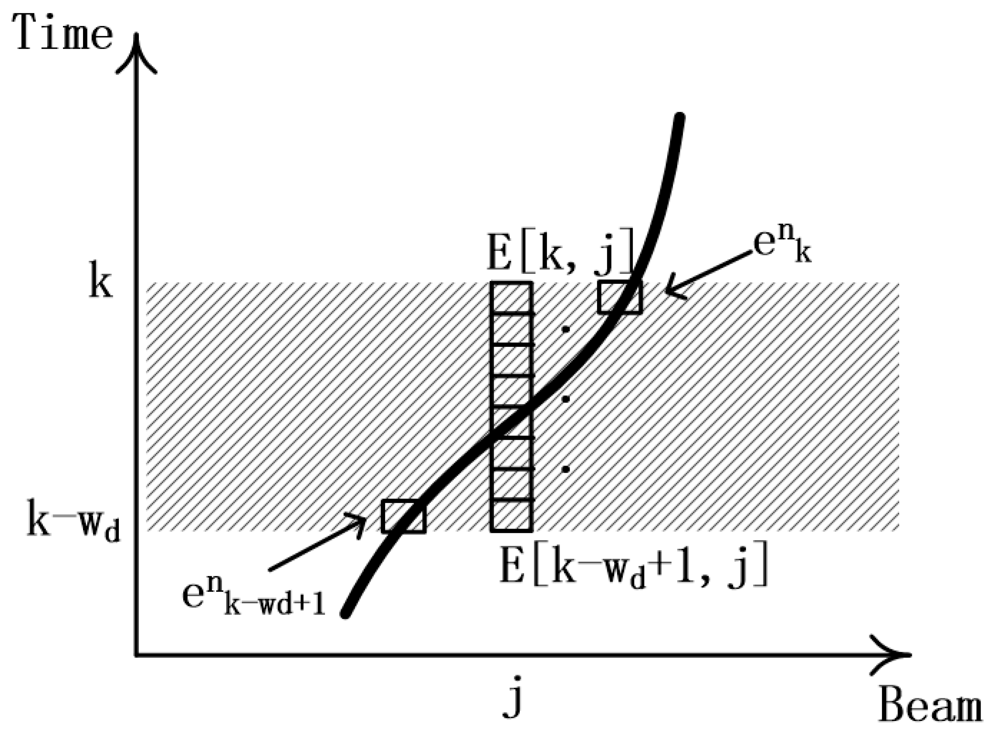
As shown in Figure 1, after being processed by beamforming, the original array element data form the Bearing Time Record (BTR), which is divided into a grid according to the beam and the moment, and the energy matrix is represented by the matrix $\mathit{E}$. $\mathit{E}[k,j_k^n]$ is an element in the matrix that represents the energy value corresponding to moment k in the orientation ${\beta }_k^n$. Let $e_k^n$ denote the energy value $\mathit{E}[k,j_k^n]$ corresponding to the azimuth at which particle $n$ is located at moment $k$. Then the energy intensity sequence of particle $n$ within the time window $k-w_d$ to $k$ is a $w_d\times 1$-dimensional vector.

$${\mathit{e}}_{k,w_d}^n={\left[e_k^n,e_{k-1}^n,\dots ,e_{k-w_d+1}^n\right]}^T$$

(15)

The energy sum of the $w_d$ scanned beams is used to define the likelihood function of the nth particle at moment k. It represents the likelihood of the particle passing through the path in $\mathit{E}$ during the time window, which is denoted by $l\left({\mathit{x}}_k^n\right|{\mathit{e}}_{k,w_d}^n)$.

$$\begin{array}{ll}\hfill l\left({\mathit{x}}_k^n\right|{\mathit{e}}_{k,w_d}^n)& ={\sum }_{i=k-w_d+1}^k{e}_i^n\\ & ={\sum }_{i=k-w_d+1}^k\mathit{E}\left[i,j_i^n\right]\end{array}$$

(16)

where $i$ is the index variable for the values between the current moment $k$ and previous moments $k-w_d$.

The integration over $w_d$ scans creates trajectories for the particles according to the motion model and accumulates energy through this trajectory. High likelihood values at long integration times indicate that the path is more consistent with the motion model, and vice versa.

The posterior probability of state can be approximated by considering the mean of the particles.

$$p\left({\mathit{x}}_k|{\mathit{Z}}_k^N\right)\approx {\sum }_{n=1}^N{w}_{k,n}^{+}\delta ({\mathit{x}}_k-{\mathit{x}}_k^n)$$

(17)

where ${\mathit{Z}}_k^n=[E_{k,w_d}^1,E_{k,w_d}^2,\dots ,E_{k,w_d}^N]$ denotes the cumulative values of all particles on their respective trajectories in the $w_d$ time window before moment k, and $w_{k,n}^{+}$ is calculated from the previous weight $w_{k,n}^{-}$ with the likelihood $l\left({\mathit{x}}_k^n\right|{\mathit{e}}_{k,w_d}^n)$.

$$w_{k,n}^{+}={\displaystyle \frac{w_{k,n}^{-}l\left({\mathit{x}}_k^n\right|{\mathit{e}}_{k,w_d}^n)}{{\sum }_{n=1}^N{w}_{k,n}^{-}l\left({\mathit{x}}_k^n\right|{\mathit{e}}_{k,w_d}^n)}}$$

(18)

The maximum or mean of the posterior probability density is often selected to obtain an estimate of the state at moment k. In this method, the mean value was calculated using the following equation:

$${\widehat{\mathit{x}}}_k={\sum }_{n=1}^N{w}_{k,n}^{+}{x}_k^n$$

(19)

An approximate state mean estimate was obtained from the above equation. In addition, the orientation tracking output ${\widehat{\beta }}_k$ for moment k can be obtained by carrying out the state estimate in Equation (12).

3. Target-Based Band Adaptive Selection

3.1. Target Beam Enhancement

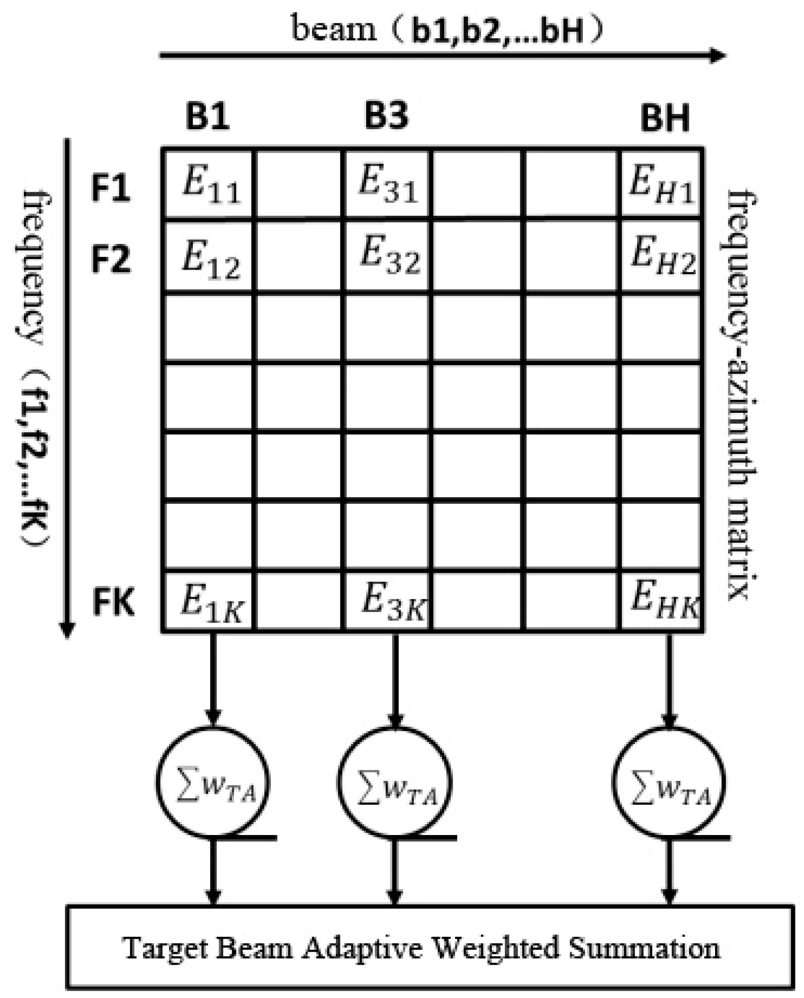
Broadband beamforming converts the received array element data into the frequency domain and then performs narrowband direction-of-arrival (DOA) estimation in several sub-bands to obtain the spatial spectrum of each narrowband. At each moment, its output is a function of the frequency and azimuth, hereafter referred to as frequency–azimuth (FRAZ) data. The FRAZ is divided into K bands and H beams, as shown in Figure 2.

Here, the output $P(f_j,b_i)$ of the $i$-th beam in the frequency band with center frequency j is

$$\begin{array}{ll}\hfill P\left(f_j,b_i\right)& ={\left|w\left(f_j,b_i\right)X\left(f_j\right)\right|}^2\\ & =w^H\left(f_j,b_i\right)R\left(f_j\right)w\left(f_j,b_i\right)\\ & =E_{ij}\end{array}$$

(20)

To enhance the target beam, the algorithm selects and acquires narrowband sub-bands based on the spectral characteristics of the signal. Specifically, the selection process involves analyzing the frequency content of the received signal to identify sub-bands that contain significant energy contributions from the target of interest.

Conventional energy detection directly sums the energy of the two-dimensional FRAZ matrix in the frequency dimension and converts it into a one-dimensional broadband spatial spectrum. The result of the $i$-th beam in the spatial spectrum $P\left(B_i\right)$ is given by the following:

$$P\left(B_i\right)={\sum }_{j=1}^{H}P\left(f_j,b_i\right)={\sum }_{j=1}^H{E}_{ij}$$

(21)

Owing to the influence of ocean background noise and platform self-noise, the noise power is larger at low frequencies, and the noise power decreases with an increase in frequency. To reduce the effect of a low-frequency background on high-frequency signals, the background noise needs to be “flattened”. The background noise is first estimated, and then the beam output is subtracted from the estimated background noise to obtain a power spectrum that is closer to the signal itself. Here, the filtered median of all beams in a certain band is used as the noise background $N_j,j=\mathrm{1,2},\cdots K$ for the current band.

$$N_j=median\left\{P\left(f_j,b_1\right),\cdots ,P\left(f_j,b_H\right)\right\}$$

(22)

3.2. Adaptive Sub-Band Selection and Weighting

Target-based adaptive sub-band selection and weighting are divided into selection and weighting processes. The band selection is to eliminate the bands with a low output signal-to-noise ratio of the target and keep only the “dominant” bands with a high output signal-to-noise ratio, while the weighting is to match the frequency features of the target and enhance the corresponding target. The output of each band is subtracted from the background estimation of the current band. The bands that account for the major energy contribution in each beam are selected, and their energy is “retained”, while the bands that are less than zero and have minimal contribution are “rejected”; that is, their output energy is set to zero. After subtracting the estimated noise from each band, the new FRAZ matrix is

$$E_{ij}\prime =\mathit{max}\left(E_{ij}-N_j,0\right)$$

(23)

where $i=1,\cdots ,H;j=1,\cdots ,K$. For each column (the same beam), the data are sorted according to the energy magnitude to obtain ${E\prime }_{is\left(j\right)}$, which gives

$$\begin{array}{c}E{\prime }_{is\left(1\right)}=\mathit{max}\left(E_{i1},E_{i2},\cdots ,E_{iH}\right)\\ E{\prime }_{is\left(H\right)}=\mathit{min}\left(E_{i1},E_{i2},\cdots ,E_{iH}\right)\end{array}$$

(24)

if $1<j<H$, then

$$E{\prime }_{is\left(j\right)}=\mathit{max}\{\left(E_{i1},\cdots ,E_{iH}\right)\backslash (E_{is\left(1\right)},\cdots ,E_{is(j-1)})\}$$

(25)

where \ denotes subtraction between sets. $E_{is\left(j\right)}^{\prime }$ is the $j$-th maximum in the series $E_{i1},E_{i2},\cdots ,E_{iH}$. For example, suppose ${E\prime }_{i1}~E{\prime }_{i5}$ equal to {1, 3, 2, 8, 6}; then, there are ${E\prime }_{is\left(1\right)}~E{\prime }_{is\left(5\right)}$ equal to {1, 2, 3, 6, 8}, with s(1) = 1, s(2) = 3, s(3) = 2, s(4) = 5, and s(5) = 4.

Define $\delta$, which satisfies

$$\left\{\begin{array}{c}\mathit{min}\delta ,\delta \in [1,H]\\ s.t.{\displaystyle \frac{{\sum }_{j=1}^{\delta }E{\prime }_{is\left(j\right)}}{{\sum }_{j=1}^{H}E{\prime }_{is\left(j\right)}}}>\Lambda \end{array}\right.$$

(26)

where $\Lambda$ denotes the percentage of retained energy of the band to be retained in the total energy of the current beam. $\Lambda$ was taken as 0.8, which means that the band contributing 80% of the energy from large to small was retained.

Based on the energy distribution of the tracking beam where a target is located, the target adaptive (TA) weights can be obtained as

$$w_{TAj}=\left\{\begin{array}{c}E{\prime }_{ij},j=s\left(1\right),s\left(2\right),\cdots ,s\left(\delta \right)\\ 0,j=s\left(\delta +1\right),\cdots ,s\left(H\right)\end{array}\right.$$

(27)

After normalization, there is

$$w_{TAj\_norm}={\displaystyle \frac{w_{TAj}}{\epsilon +{\sum }_{j=1}^H{w}_{TAj}}}$$

(28)

where $\epsilon$ is an extremely small value to avoid a zero denominator. The target adaptive selection weighted output for beam $B_i$ is expressed as

$$P_{TA}\left(B_i\right)={\sum }_{j=1}^H{w}_{TAj\_norm}·E{\prime }_{ij}$$

(29)

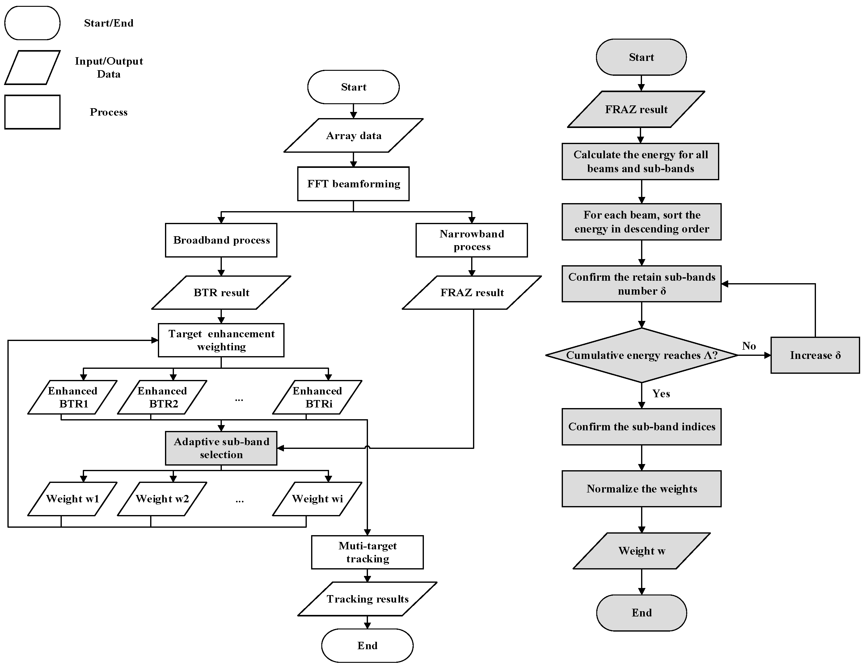
The algorithm flowchart is shown on the right side of Figure 3.

3.3. Adaptive Nature of the Algorithm

The adaptivity of the algorithm is reflected in its capability to dynamically adjust the frequency-band selection and weight allocation in response to the real-time characteristics of the target. At each time step, the algorithm acquires the azimuth from the tracking results and dynamically identifies the energy distribution of the target across the different frequency bands. Subsequently, it selects the “dominant” frequency bands with a high signal-to-noise ratio and assigns them higher weights, while rejecting frequency bands with a low signal-to-noise ratio. This dynamic adjustment ensures that the algorithm can adapt to changes in the target’s characteristics and environmental noise, thereby enhancing the continuity and accuracy of the target tracking.

Figure 3 shows the processing structure, which combines the target-tracking output with the “matching and weighting” of band features for different targets to obtain the corresponding spatial spectrum to improve the tracking of weak targets. The rectangular blocks represent processing steps; the quadrilateral blocks represent data; and the rounded rectangles indicate the start or end of the process.

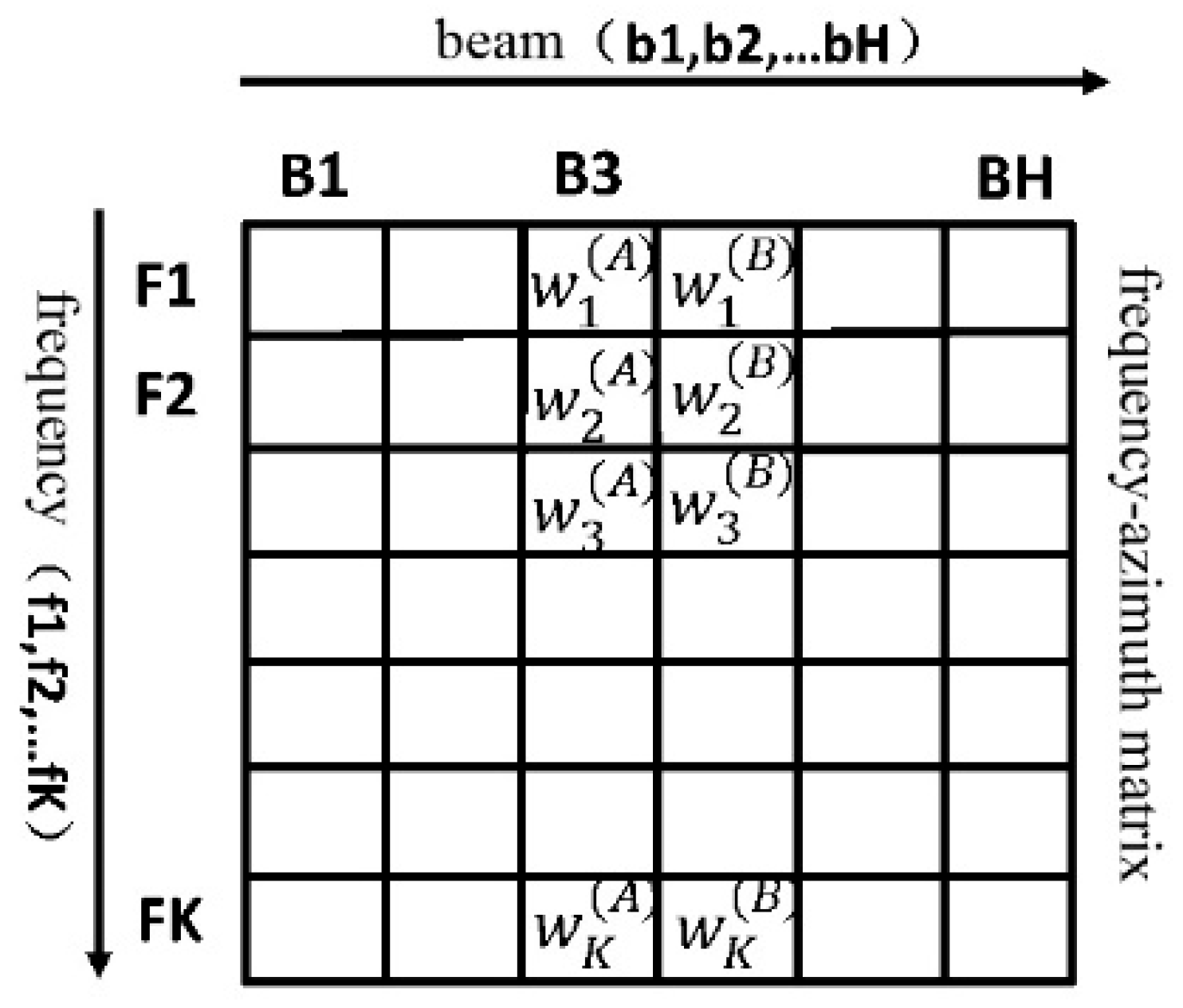
The adaptivity of the algorithm is further enhanced by its ability to adjust weights during the target crossovers. When two targets cross each other, the algorithm calculates separate weights for each target based on their respective band features. These weights are then used to perform spatial spectral weighting on each target, allowing the algorithm to distinguish between the two targets even when they overlap in the azimuth. This dynamic weight adjustment during the crossovers further improves the robustness of the tracking process.

When two targets A and B are at crossover, high weights are given to those bands that contribute major energy to target A and little to target B, and zero weights are additionally given to those bands that contribute major energy to B and little to A. In this way, the broadband summation can strengthen target A while suppressing target B and improve the signal-to-interference ratio of target A with respect to target B, and vice versa.

A schematic diagram of cross weighting is given in Figure 4, in which targets A and B will cross in azimuth, and the latest normalized weights $w^{\left(A\right)}$ and $w^{\left(B\right)}$ have been obtained before the crossover based on their respective band features, given by Equation (30).

$$\begin{array}{c}{\sum }_{j=1}^K{w}^{\left(A\right)}=1\\ {\sum }_{j=1}^K{w}^{\left(B\right)}=1\end{array}$$

(30)

Then during the crossover, the cross weights $w^{\left\{A\right\}}$ and $w^{\left\{B\right\}}$ are used to perform spatial spectral weighting on target A and target B, respectively. $w^{\left\{A\right\}}$ and $w^{\left\{B\right\}}$ are given by

$$\begin{array}{c}{w}_j^{\left\{A\right\}}={\displaystyle \frac{\mathit{max}\left(w_j^{\left(A\right)}-w_j^{\left(B\right)},0\right)}{{\sum }_{j=1}^K\mathit{max}\left(w_j^{\left(A\right)}-w_j^{\left(B\right)},0\right)}} \\ w_j^{\left\{B\right\}}={\displaystyle \frac{\mathit{max}\left(w_j^{\left(B\right)}-w_j^{\left(A\right)},0\right)}{{\sum }_{j=1}^K\mathit{max}\left(w_j^{\left(B\right)}-w_j^{\left(A\right)},0\right)}}\end{array}$$

(31)

where $w_j^{\left\{\mathrm{A}\right\}}$ and $w_j^{\left\{\mathrm{B}\right\}}$ are the weighted weights used for the two targets during crossover. The $w_j^{\left(\mathrm{A}\right)}$ and $w_j^{\left(\mathrm{B}\right)}$ are the last updated adaptive target weights before target crossover, where $j=\mathrm{1,2},\cdots ,K$.

For more than two targets, the algorithm extends the weight-adjustment rule by iteratively applying the cross-weighting scheme to each pair of targets. Specifically, the algorithm first determines which target’s characteristic sub-band each sub-band belongs to and then calculates the cross weights as described previously, until the weights for all targets are adjusted. The final weights for each target are normalized to ensure that the sum of weights for all targets in each frequency band equals one.

$$\begin{array}{c}{w}_j^{\left\{A\right\}}={\displaystyle \frac{\mathit{max}\left(w_j^{\left(A\right)}-max(w_j^{\left(B\right)},w_j^{\left(C\right)}),0\right)}{{\sum }_{j=1}^K\mathit{max}\left(w_j^{\left(A\right)}-max(w_j^{\left(B\right)},w_j^{\left(C\right)}),0\right)}} \\ w_j^{\left\{B\right\}}={\displaystyle \frac{\mathit{max}\left(w_j^{\left(B\right)}-\max \left(w_j^{\left(A\right)},w_j^{\left(C\right)}\right),0\right)}{{\sum }_{j=1}^K\mathit{max}\left(w_j^{\left(B\right)}\max \left(w_j^{\left(A\right)},w_j^{\left(C\right)}\right),0\right)}}\\ w_j^{\left\{C\right\}}={\displaystyle \frac{\mathit{max}\left(w_j^{\left(C\right)}-\max \left(w_j^{\left(A\right)},w_j^{\left(B\right)}\right),0\right)}{{\sum }_{j=1}^K\mathit{max}\left(w_j^{\left(C\right)}\max \left(w_j^{\left(A\right)},w_j^{\left(B\right)}\right),0\right)}}\\ \end{array}$$

(32)

The adaptivity of the algorithm is crucial for maintaining tracking continuity, particularly when weak targets cross paths with strong ones. By dynamically selecting and weighting the frequency bands based on the real-time energy distribution of the target, the algorithm can effectively reduce the impact of strong interference on weak targets, thereby minimizing tracking discontinuities and improving the overall tracking performance. This adaptivity makes the algorithm highly suitable for complex underwater acoustic environments, in which the target characteristics and interference levels can change rapidly.

4. Experiments and Analysis

The proposed joint algorithm was verified using sea-test data. The experimental data were sourced from a linear array mounted on the UUV platform. During the experiment, the UUV platform moved in a straight line at a speed of 4 knots. The array aperture is 8 m, and the data processing utilizes the received data from 32 array elements. Broadband beamforming is performed in the frequency band of 1 kHz to 3 kHz, and the band is divided into 400 sub-bands for narrowband beamforming. This array converts the received signals into FRAZ data via narrowband DOA processing. The FRAZ data were further processed through broadband integration and summation to generate the BTR, which served as raw data for the tracking algorithm.

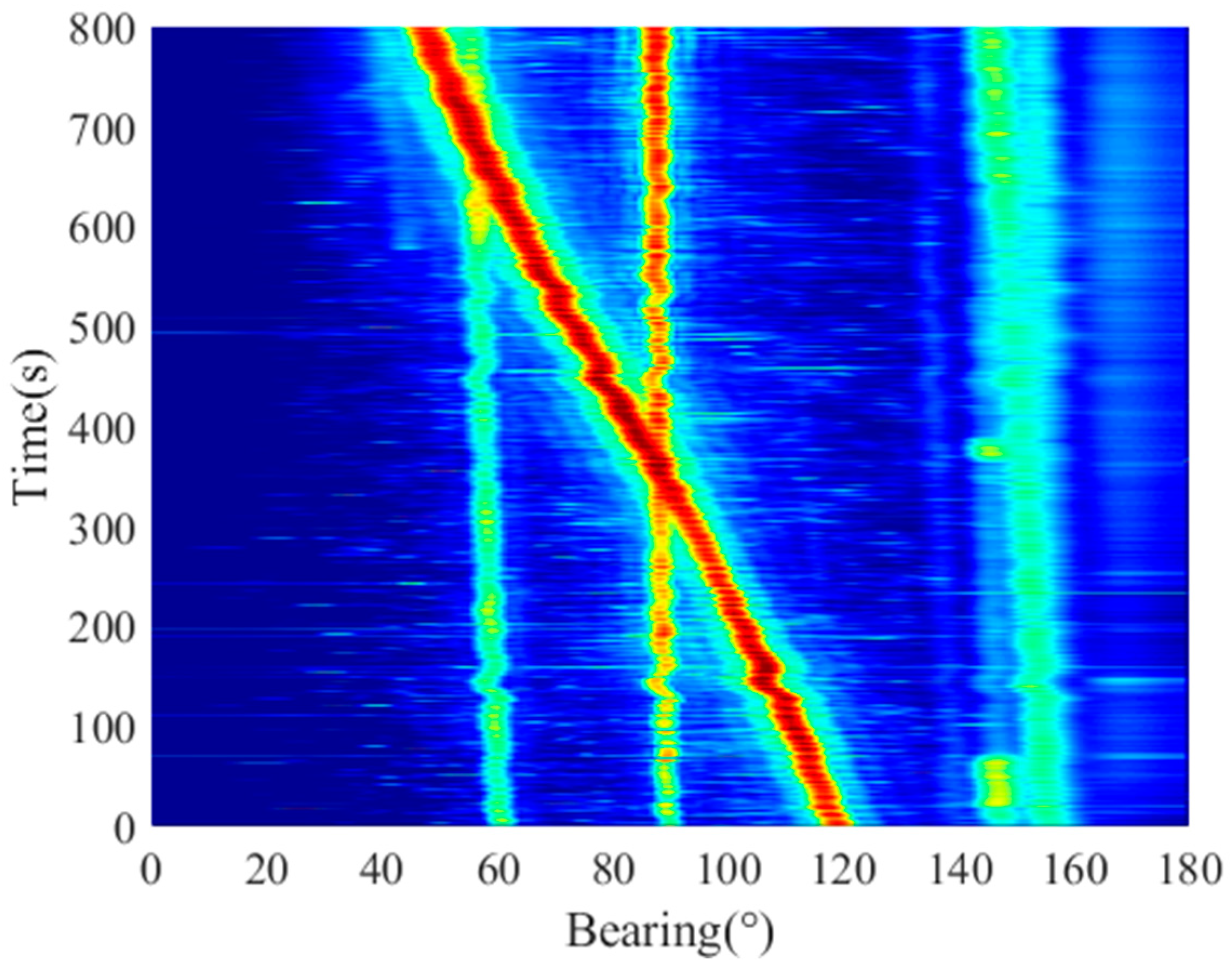
The angle of incidence of the signal was defined as 0° in the bow direction and 180° in the stern direction. The (0°, 180°] grid was scanned using linear array data with a scan interval of ∆θ = 1° and a frame duration of 1 s. The broadband BTR obtained using conventional beamforming in the working frequency band is shown in Figure 5.

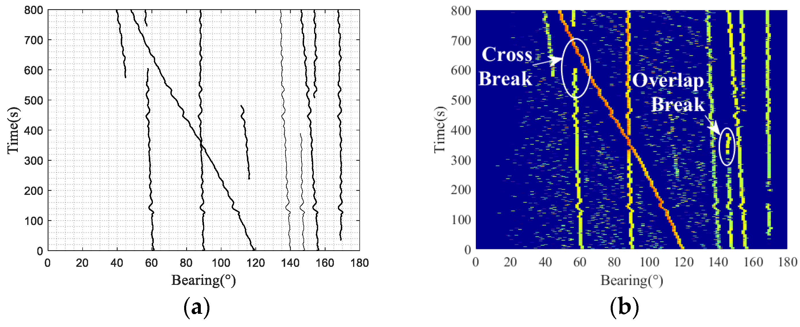
The state transfer equation of the target was constructed using the constant velocity (CV) model. The BTR in Figure 5 was tracked using the particle filtering algorithm based on energy likelihood. The initial number of particles was 2000 for each target, and the initial azimuth was randomly distributed within ±0.5° of the target peak azimuth. The distance states of the particles were randomly distributed in the range 0.1~10 km. The velocity states of the particles were randomly distributed in the range 0~10 m/s, depending on the specific situation. The heading of each particle was randomly distributed in the range of 0~360°. The tracking results are shown in Figure 6a.

The tracking results show that the tracking of a target with an azimuth of 60° was interrupted when it crossed at 650 s. At 600 s, the algorithm determined that the track had terminated, and after the end of the target crossing, it determined the start of the track again at 750 s. The prolonged disappearance of weak targets leads to discontinuities and changes in trackers. After 400 s, the target with an azimuth of 150° gradually overlaps the right target. The algorithm determines that the track is terminated, and the target is lost at approximately 400 s.

The above results were further analyzed. During the tracking process, targets with azimuth angles varying from 120° to 50° have stronger energy. The two targets with azimuths of 90° and 60° have relatively weak energy, so the peak is affected during the crossover. The target at 60° was affected for a longer period of time because of its weaker intensity. The peak result is shown in Figure 6b, which indicates that the peak of the weak target was interrupted by the interference of the strong target during the crossover from 600 s to 700 s. The peak interruption of the weak target leads to the determination of track termination before entering the crossing state; therefore, the tracking of the crossing target cannot be performed correctly. However, the target crossover at 350 s can correctly predict the target trajectory based on the particle state because of the small energy intensity difference between the targets and the short peak missing time. Because the target with an azimuth angle of 150° overlaps with the right target in azimuth for a long time, there is only one peak after 400 s; therefore, it is determined that the track is terminated.

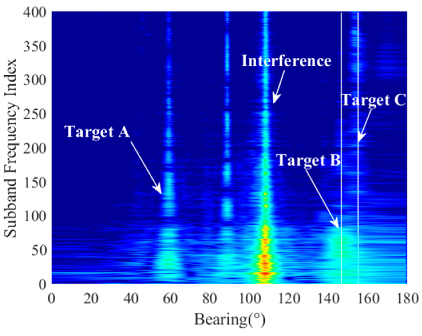
The frequency-band adaptive selection method based on tracking targets can use the concept of frequency-band matching to strengthen the target being tracked while weakening the target that crosses it. This method enhances the continuity of target peaks and allows for direct distinction of crossing targets by frequency when there are differences in their frequency—band characteristics. The initial FRAZ is shown in Figure 7. The target with an initial azimuth of 60° is defined as target A, and targets with azimuths of 150° and 160° are defined as targets B and C, and the strong interference is initially at 110°. It can be observed that there are significant differences in the intensity distribution of the target in terms of frequency. The strong interference has an equal energy distribution in each frequency band, so it overwhelms target A in the crossover process. Target B has a strong concentration of energy in the band of serial numbers 50~100 and almost no energy in the band of serial numbers 300~400. However, target C, which overlaps with target B for a long time, has a strong SNR in the band of serial numbers 300~400.

The joint processing of band features and particle state features was used to track target A. First, the band features of the tracked target were obtained based on the azimuth tracking results of the particle filtering. Second, the target band adaptive weighting vector is calculated, and the enhanced spatial spectrum of the tracked target is used for the subsequent tracking of target A. Finally, the new weights are calculated again from the tracking results.

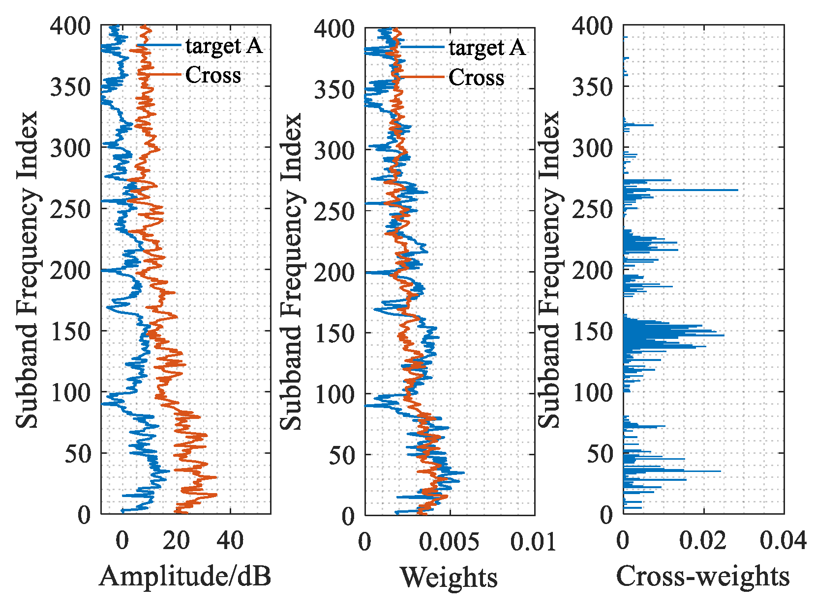
Figure 8 illustrates the band adaptive weight assignment results for target A during crossover, revealing the key advantages of the proposed method in handling the intersection of target signals and strong interference. From left to right, the figure displays the energy distribution of target A and the interference, as well as the matching weights calculated based on their respective spectral distributions. The energy distribution across sub-bands shows that target A’s energy is weaker than the interference in all the analyzed bands, resulting in a signal-to-interference ratio (SIR) of less than 0 dB. However, target A exhibits a relatively higher SIR in some sub-bands. The weight distribution of target A and the interference indicates that target A has a certain “dominance” in sub-bands numbered 125–150 and 220–240, where the SIR is relatively higher. By enhancing target A’s relative “dominance” in these sub-bands, the proposed method not only effectively improves the detectability of the target signal but also maintains signal continuity during the crossover period. This dynamic weight allocation strategy is one of the core innovations of the proposed method, enhancing target detection performance in complex interference environments.

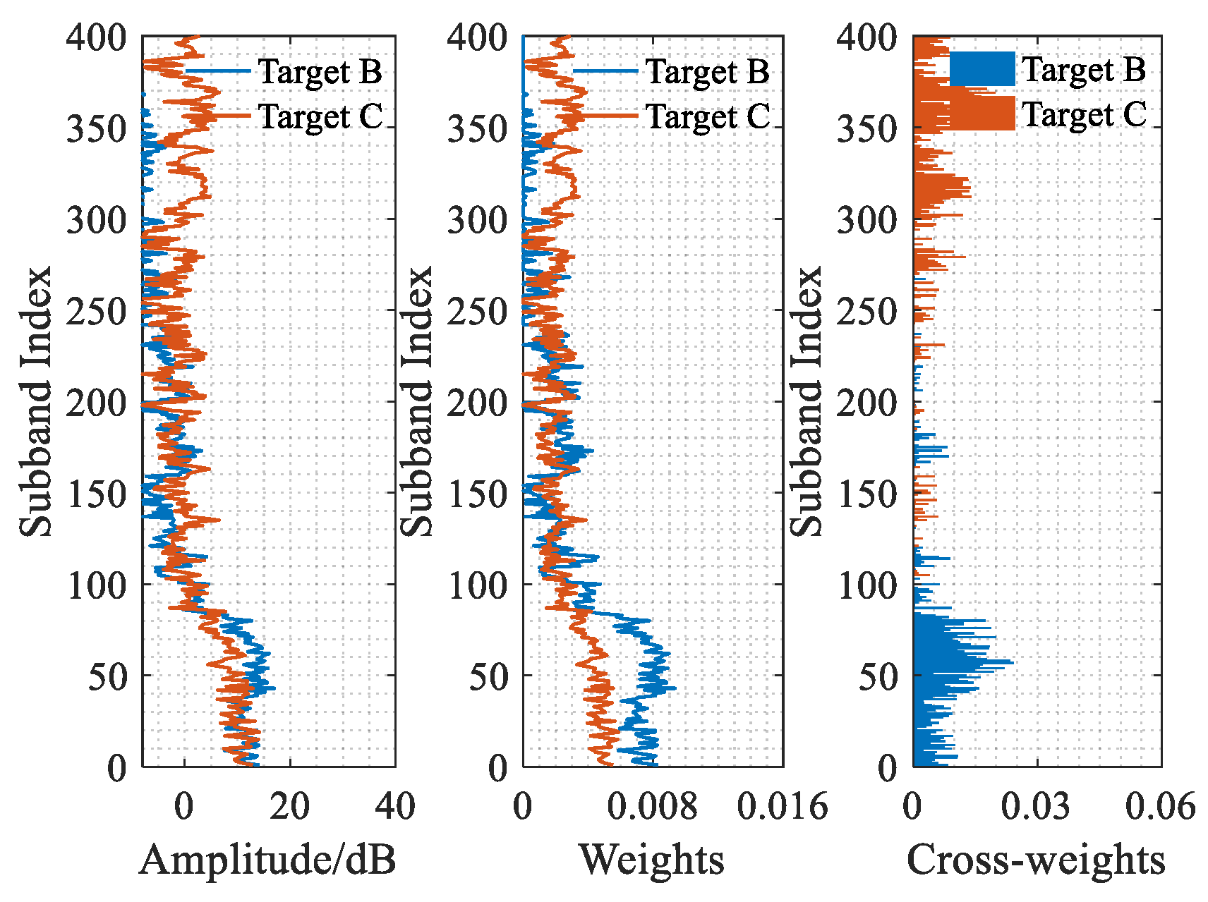
Similarly, the results of the joint processing of objectives B and C are shown in Figure 9. The cross weights of target B and target C during the overlap period show that the “strong” sub-band of target B is in the top 100 sub-bands, while the “strong” sub-band of target C is between 300 and 400. When the same BTR is used as the tracking input, the two targets overlap in azimuth, and only one target can be tracked. However, by weighting according to the cross weights to obtain the BTR for target B and the BTR for target C, it is easy to distinguish the two targets on the same azimuth and provide correct tracking results during the overlap.

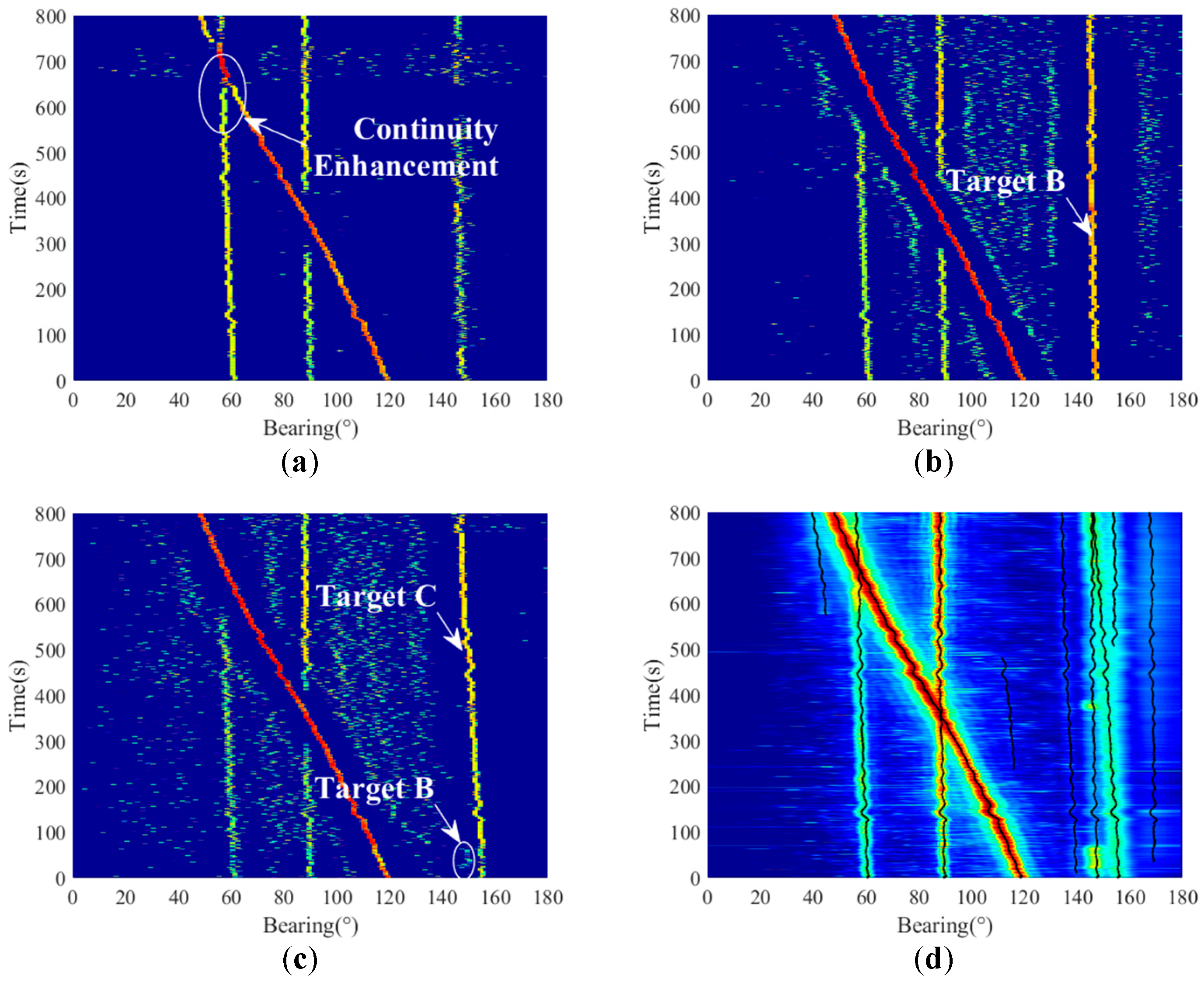
Figure 10a–c show the sub-band adaptive weighting results of the peak history for targets A, B, and C, respectively. The processing results were compared with the original BTR to obtain Figure 10d.

To demonstrate the superiority of our proposed algorithm, we compared it with the traditional detect-before-track (DBT) [7], Standard PF-TBD [8], and recent state-of-the-art methods including deep learning TBD (DL-TBD) [24]. In traditional DBT following Bar-Shalom’s framework [7], the measurements were thresholded at the 3σ noise level before Kalman filtering with nearest-neighbor association. Standard PF-TBD was implemented according to Arulampalam’s particle filtering guidelines [8] with 2000 particles and energy likelihood matching. The DL-TBD adopted Wang et al.’s CNN architecture [24] trained on our dataset with identical input BTRs.

For a fair comparison, all the particle-based methods used identical resampling thresholds (set resampling thresholds < 50%) and systematic resampling with 2000 particles and energy likelihood matching. The DP-TBD implementation followed [26], trained on our dataset with identical input BTRs with a grid resolution of Δθ = 0.5°. All the timing metrics were obtained on an Intel i7-11800H CPU using a single-threaded MATLAB 2018b implementation.

The results in

Table 1. Comparison of tracking performance among different algorithms.

Algorithm	Tracking Accuracy (RMSE°)	Trajectory Continuity (%)	Computational Complexity (ms)
Traditional DBT [7]	2.75 ± 0.31	62.3	15.2
PF-TBD [8]	1.89 ± 0.25	78.1	82.7
DL-TBD [26]	1.52 ± 0.18	82.4	136.5
Proposed Method	0.93 ± 0.11	93.2	105.3

show that we adopted the following methods to calculate the tracking accuracy and trajectory continuity metrics. The tracking accuracy was quantified using the root mean square error (RMSE) between the estimated and ground-truth positions (obtained via GPS-augmented surface buoy markers). Trajectory continuity was measured as the percentage of time steps without track fragmentation (>3 s gaps). The computational complexity was evaluated via the processing time/frame (ms) on an Intel i7-11800H CPU.

To isolate the contribution of sub-band weighting, we conducted ablation tests by removing the adaptive weighting module. This resulted in an RMSE degradation from 0.93° to 1.64°, confirming the critical role of band adaptation.

The proposed method reduces tracking discontinuity compared with conventional PF-TBD (from 78.1% to 93.2%) while maintaining real-time capability (<150 ms/frame). Frequency-domain feature weighting proved particularly effective during target crossovers in which we observed a reduction in track swaps. The current implementation requires a predefined target count. Future work will integrate birth/death processes and explore GPU acceleration for >10,000 particles.

5. Conclusions

This paper presents a novel TBD algorithm that integrates particle states and band features to enhance the tracking of weak targets in complex underwater acoustic environments. By introducing frequency-band adaptive matching and particle filter techniques, the algorithm significantly improves the continuity and accuracy of target trajectories, especially in scenarios in which targets cross paths. The experimental results, supported by detailed hardware setup and data processing, demonstrate the robustness and effectiveness of the proposed method.

However, the proposed algorithm also has notable limitations. It does not account for the birth and death of targets, and the added frequency-band adaptation and particle filtering processes increase the computational complexity. Additionally, the algorithm’s performance has only been validated in a single array configuration and a specific marine environment. To address these limitations, future work will introduce dynamic birth and death processes to handle changes in the number of targets. We will continue to explore optimization strategies, such as GPU acceleration and the use of lower-resolution sub-bands, to reduce processing time while maintaining tracking performance. Furthermore, the algorithm will be tested in multiple sonar configurations and environments to assess its robustness and adaptability.

In summary, although the proposed algorithm achieves high tracking accuracy and continuity, addressing its current limitations is crucial for enhancing its practicality and robustness. Future efforts will focus on optimizing the algorithm to reduce computational complexity while preserving its performance advantages, making it more suitable for real-world applications in complex underwater environments.