Article

Modeling Pulsed Magnetic Core Behavior in LTspice

1
Center for Pulsed Power and Power Electronics, Texas Tech University, Lubbock, TX 79409, USA
2
Nevada National Security Sites, Las Vegas, NV 89193, USA
*
Authors to whom correspondence should be addressed.
Electronics 2025, 14(12), 2335; https://doi.org/10.3390/electronics14122335
Submission received: 29 April 2025 / Revised: 24 May 2025 / Accepted: 5 June 2025 / Published: 7 June 2025
(This article belongs to the Special Issue Advances in Pulsed-Power and High-Power Electronics)

Abstract

This work demonstrates a modeling technique focused on reproducing the behavior of magnetic cores subject to high voltage pulses. The working principle of the model is based on a magnetic circuit with additional elements that influence the model’s behavior. The elements include a function that defines the response of the model depending on the applied pulse voltage and a component that dominates the transient response. These elements are necessary to replicate the experimentally observed behavior of magnetic cores. The model was developed based on the measured behavior of three nanocrystalline magnetic materials subject to a range of pulse voltages. This modeling technique was created to address the limitations of other models in accurately capturing fast pulse responses. The key limitation of traditional modeling techniques that the proposed model addresses is their inability to capture variations in core response under different applied pulse voltages (magnetization rates). The proposed model has been shown to produce accurate results for magnetization rates between 1 T/μs and 8 T/μs, with potential for further expansion. Implemented in LTspice, this model is both fast and accurate, effectively replicating the behavior of the magnetic core while maintaining simplicity. This work outlines the foundation of this modeling technique, the trends in the parameters that influence its behavior, and its application within a simple pulsed power system. The most notable feature of this model is its ability to operate across a wide range of pulse voltages without requiring adjustments to the model parameters.

1. Introduction

Nanocrystalline and other complex magnetic materials have been developed with advantageous properties for many applications, particularly pulsed power systems with a high pulse voltage output [1]. The large relative permeability of these materials and their thin laminations are their main advantage, allowing them to have low losses compared to other core types. While these attributes enable them to behave better than alternative materials, modeling them presents several challenges. Generally, the information available on these magnetic materials is given in the context of low-frequency AC systems. Although these low-frequency properties influence the core behavior under pulsed excitation, accurately extrapolating the exact magnetic core response remains challenging.
Currently, several magnetic core modeling techniques are available. Common lumped circuit techniques are the Jiles–Atherton and the Chan models. Alternatively, computationally expensive 2-D and 3-D numerical physics approaches are options and have their challenges and limitations. Another option, the magnetic circuit model, also a lumped circuit approach, is exploited in the presented work.
The Jiles–Atherton approach is an accurate model that utilizes a set of constants to model the major and minor hysteresis loops [2]. These constants are not well known based on the properties provided by the magnetic material manufacturer. They must be found by iteratively solving differential equations numerically [3]. Another challenge with the Jiles–Atherton model is its difficult implementation in standard circuit simulation software, like LTspice, where it is not readily supported. The LTspice native saturable inductor models magnetic hysteresis based on the Chan model [4]. Two different equations calculate B based on whether H is increasing or decreasing. This model also handles minor hysteresis loops well, where the minor loops only reach within the major hysteresis loop [5]. The LTspice saturable core model conveniently uses parameters commonly provided by magnetic core manufacturers, such as the saturation magnetic flux density, Bs, remnant magnetic flux density, Br, and the magnetic coercive force, Hc. However, there are drawbacks to this technique, the largest being the lack of frequency dependence of the hysteresis curve in the LTspice implementation of the model. This leads to significant errors in the hysteresis curve at high frequencies and in pulsed applications since the hysteresis curve widens significantly with increasing frequency or increased pulse voltage. The Chan model is most suitable for ferrite materials with less-square hysteresis loops than the nanocrystalline and amorphous cores typically used in pulsed power systems [6]. It is also ideal for the constant frequency operation of the core, where the B-H curve remains fixed rather than dynamic, as it is in pulsed scenarios.
Many commercially available 2-D and 3-D multi-physics simulators support magnetic core modeling. However, they are best suited for low-frequency systems. In high-frequency or pulsed systems, microscopic phenomena within laminations become significant and must be resolved. This results in a computational domain with a mesh that is much too fine to resolve. To alleviate this issue, ref. [7] suggests manipulating the magnetic material’s physical properties to reproduce the magnetic core’s actual behavior with a manageable domain mesh size. Even with these adjustments, simulation run-time is still a significant concern in large-scale systems. An alternate modeling technique based on a magnetic circuit is outlined in [8]. This technique features a DC hysteresis component and the losses in a magnetic circuit. Although the model gives a straightforward method of producing the losses of a magnetic core derived from known magnetic core parameters, it was found that the model proposed in [8] fails to align well with the experimental data for fast-pulsed excitations of nanocrystalline magnetic cores.
The presented approach introduces an alternative modeling technique to the more commonly used models, which have limitations in high-voltage systems with fast rise times. Implemented in LTspice XVII (version 17.1.15, Analog Devices, Norwood, MA, USA), this core modeling technique uses a magnetic circuit to replicate the behavior of magnetic cores at high magnetization rates with just a few input parameters. The presented model accurately replicates the B-H curve widening and experimental results across various pulse voltages, making it ideal for dynamic systems. Additionally, it benefits from minimal computational time, enabling a rapid pulsed power design process.

2. Materials and Methods

2.1. Background

2.1.1. Magnetic Hysteresis

Magnetic hysteresis describes the relationship between the magnetic flux density, B, and the magnetic field, H. Magnetic hysteresis is modeled using the Jiles–Atherton approach in [3], whereas the foundation of another method, the Chan model, is described in [4] and its application within a circuit simulation software is outlined in [5]. Additionally, the work presented in [8] introduces a technique utilizing the magnetic circuit approach to model magnetic hysteresis. Each of these methods focus on relatively low-frequency systems, especially when compared to the 100 s of nanosecond to several microsecond pulse durations of interest in this work. In such systems, the magnetization rate is sufficiently low that the entire magnetic core maintains nearly uniform B and H values at any moment. However, in high-frequency and pulsed systems, the finite magnetic field diffusion time becomes a dominant factor in the core response. A method of estimating the losses for high-frequency systems working below saturation has been proposed in [9]. This finite diffusion time results in regions of the magnetic core being saturated while other areas have very low B-fields, revealing the true 3-D nature of the magnetic core.
Generally, the hysteresis curve of a magnetic core is derived from Faraday’s law and Ampere’s law, which are defined by the following equations.
B t = 1 N · A e V t d t
H t =   N · i ( t ) l e
where V(t) denotes the voltage measured across the magnetic core, N denotes the number of turns, Ae denotes the effective area of the magnetic core, le denotes the length of the average magnetic path through the core, and i(t) denotes the current through the windings of the magnetic core. It has been seen experimentally that the hysteresis curve widens with an increase in frequency or magnetization rate in the pulsed case [10,11,12,13]. Assuming a square pulse, the magnetization rate is obtained by differentiating Equation (1),
d B d t =   V N · A e
The broadening of the hysteresis curve is significant for several reasons, one being the energy loss associated with the area within the hysteresis loop, given by the following equation.
E l o s s m 3 = H d B
Equation (4) gives an expression for magnetic core loss per unit volume, having the unit J/m3. In many applications, such as transformers and pulse compression devices, minimizing energy loss is crucial. Additionally, a broader hysteresis curve typically features a lower effective permeability and, thus, a lower impedance of the magnetic core, which is often undesirable.
Note that the above equations are based on an average of the magnetic field across the entire magnetic core. This is not an issue for low magnetization rates since the field amplitudes would be roughly homogeneous. However, as soon as high magnetization rates are considered, one can only deduce an effective B-field from Equation (1) and must keep in mind that there are regions of high and low magnetic field amplitudes in the core. Consequently, a widening of the B-H curve determined from Equations (1) and (2) is observed experimentally when the magnetization is non-uniform in the core. This effect seems dominant and different from the increasing B-H curve area due to finite magnetic domain alignment speeds and domain wall processes important on the single-digit nanosecond timescale [14].

2.1.2. Experimental Setup

A pulser board was developed to experimentally evaluate the behavior of magnetic cores subject to pulsed voltages of up to 2.5 kV with a peak pulsed current of 200 A. The pulser utilizes SiC MOSFETs, allowing rise times of around 25 ns. Considering the size of the cores and the capability of the pulser board, most testing was performed with two windings to achieve the magnetization rates of interest (1 T/μs–8 T/μs) and ensure the sufficient saturation of the magnetic core.
Current and differential voltage are measured on the pulse-exciting two-turn winding (see Figure 1). A reset winding is employed to consistently reset the core to its initial remnant magnetization, allowing for comparisons at different pulse voltages and between various magnetic cores. In developing this modeling technique, three nanocrystalline magnetic core types were evaluated, all made by the same manufacturer, FINEMET (Proterial Ltd, Tokyo, Japan). The three magnetic core materials are FT-3KM, FT-3K50T, and FT-3KL. The cores have a similar composition, but their magnetic properties differ significantly. See Table 1 for details concerning these differences due to the annealing techniques used for each one. Since these magnetic cores are essentially the same size and shape, they can be directly compared. For reference, the cores have an OD of 79 mm, an ID of 51 mm, and a height of 25 mm.
While the saturated magnetic flux density is the same for all three cores, there appears to be a trade-off between remnant magnetization and DC permeability. One may postulate that this trade-off prevents creating a material with a low Br and a high μr. This proposed model aims to accurately capture the widening of the hysteresis curve seen experimentally across a range of magnetization rates often seen in pulsed power systems and evaluate the influence of the magnetic core parameters given in Table 1 on the model input parameters.

2.2. Magnetic Core Model Fundamentals

The working principle of this magnetic core modeling scheme employs an equivalent magnetic circuit that simulates the behavior of a saturable magnetic core in the electrical domain.
In the magnetic circuit, the magnetomotive force (mmf) is expressed by the current through the inductor multiplied by the number of turns, N; see the right side of Figure 2. The magnetic equivalent of electrical resistance is reluctance, which depends on the geometry and permeability of the magnetic core. Finally, the electric current equivalent in the magnetic circuit is magnetic flux. The expression for magnetic flux in this magnetic circuit is as follows.
Φ = N · I R = N · I · μ · A e l e
where N represents the number of turns on the primary winding, I represents the current through the primary windings, μ represents the permeability of the magnetic core, Ae represents the effective area of the core, and le represents the length of the closed-loop magnetic path of the core. The voltage across the magnetic core can be found through Faraday’s law of induction, which is as follows:
V = N d Φ d t
This voltage is the potential across the magnetic core and can be modeled as a behavioral voltage source. In building the foundation of this modeling scheme, it is initially assumed that the permeability of the magnetic core is constant. Thus, the voltage across the core can be written as follows:
V = N 2 · μ · A e l e d I d t
The inductance of a long solenoid or toroidal magnetic core can be expressed as follows:
L = N 2 · μ · A e l e
From Equations (6) and (7), it is shown that this technique adequately models an inductor. This forms the basis of magnetic core modeling as a magnetic circuit. Implementing the above equations in LTspice as circuits in the magnetic and electric domain forms the foundation of this magnetic core modeling technique. The model has several input parameters dependent on the magnetic core geometry and magnetic properties that influence the model’s behavior. These parameters are the effective area of the magnetic core, the magnetic length, and the permeability of the magnetic core.

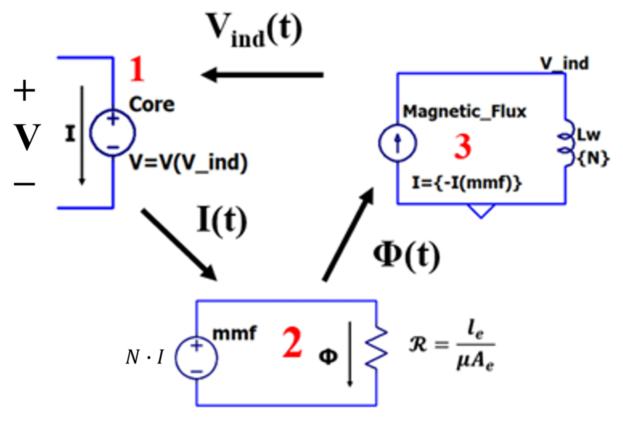
2.3. Core Model Implementation in LTspice
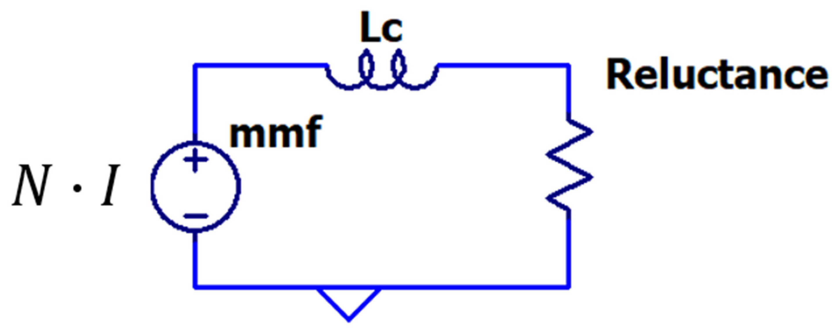
2.3.1. Basics

Implementing this model in its most basic form comprises three components: the magnetic core in the electric circuit domain, the magnetic circuit, and the induced voltage that unifies these two through Faraday’s law of induction. The model utilizes several behavioral voltage and current sources as inputs to each circuit dependent on the other subcircuits of the model, ensuring a self-consistent system.
The model components depicted in Figure 3 are (1) the magnetic core seen from the electrical side, (2) the magnetic circuit, and (3) the induced voltage fed back to the electrical circuit side. The magnetic circuit takes the current through the magnetic core as an input. This current, multiplied by N, the number of turns on the exciting winding, gives the magnetomotive force of the magnetic circuit. The magnetomotive force drives the magnetic circuit and produces a magnetic flux limited by the reluctance. This magnetic flux produces an induced voltage of V i n d = N d Φ d t . In subcircuit (3), the induced voltage is achieved with a series inductor with a value of N through V i n d = L d ( I ) d t . Finally, the magnetic core is modeled as a behavioral voltage source with V = V i n d . The model described above may be found in other sources, for instance, in [15]. Still, it is reiterated as it forms the foundation for the modifications and additions discussed in the following sections that enable the simulation of pulsed power cores.

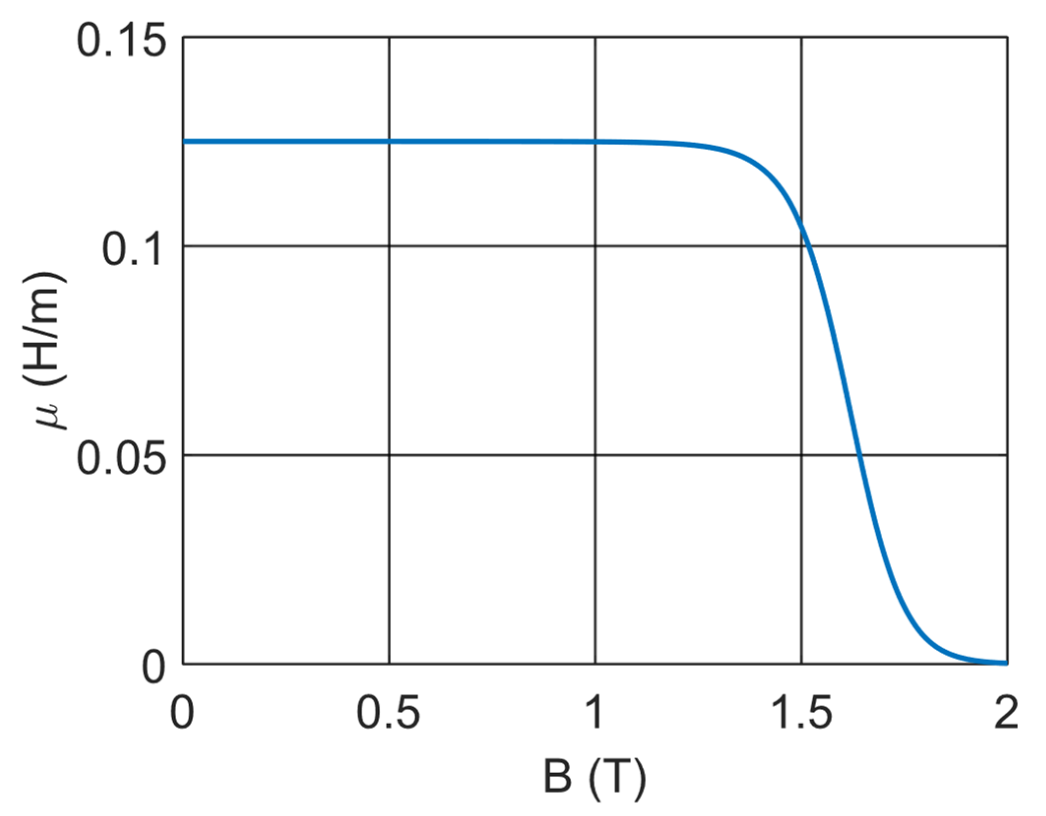
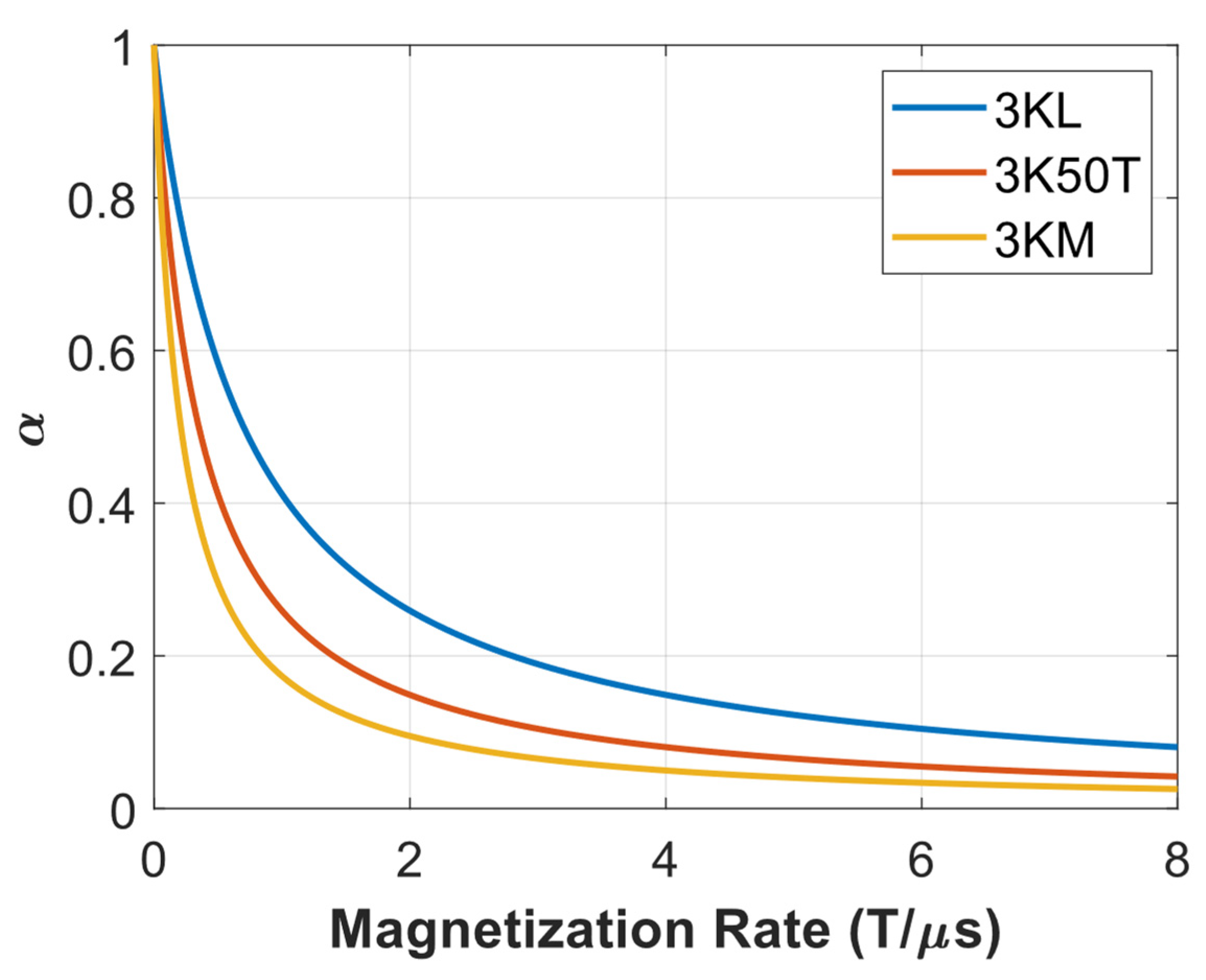
2.3.2. Core Behavior Modulation

The saturation effects of the model are represented by Brauer’s curve, which presents permeability as a function of the magnetic flux density. This function produces a relatively constant permeability until saturation, where the permeability transitions towards μ0. The following equation represents Brauer’s curve [16].
μ ( B ) = k 1 · e k 2 · B 2 + k 3 1
where B = Φ A e gives the magnetic flux density, and k1, k2, and k3 represent the constants that influence the shape of the produced curve. Through the manipulation of the k parameters, an approximate DC hysteresis curve for a given magnetic material can be produced by fitting the curve to the known or measured DC or low-frequency B-H curve. Figure 4 shows the permeability curve generated using Brauer’s model, which was matched to the DC permeability curve of the FT-3KM material. Experience indicates that measuring the B-H curve at 60 Hz yields proper results. The B dependence of this permeability curve is squared. Thus, the model is equipped for unipolar or bipolar operations. Other functions, such as a hyperbolic secant function squared, can also produce a functional permeability curve.
This permeability curve represents the microscopic/uniform field distributed behavior of the magnetic core, and the following outlines how deviation from this behavior due to non-uniform field distribution and other microscopic processes is modeled. It is important to note that this permeability curve does not account for the initial low permeability associated with the coercive magnetic field; instead, this approach gives the maximum permeability of the materials until saturation. A different method accounts for the contributions from the width of the DC hysteresis curve. In addition to the core saturation, the model must replicate the expansion of the hysteresis curve observed experimentally. The widening effect has two distinct components that can be controlled independently to produce a wide range of hysteresis curves and accurately model the behavior of different core materials.
Two features of the hysteresis curve may be manipulated as follows. The slope signified in Figure 5 is influenced by the manipulation of the reluctance of the magnetic circuit, which limits the magnetic flux. Consequently, an increase in reluctance decreases effective permeability, defined by the equation μ e f f = d B d H . The modified reluctance is given simply by R = R α , where is the reluctance found previously. The relationship between magnetization rate and α was found by adjusting α to match experimental hysteresis curves at different magnetization rates for all three magnetic cores. Each of these relationships was then fitted with a rational fit function given by Equation (10).
α d B d t = 1 1 γ · d B d t + 1
where dB/dt denotes the magnetization rate in (T/μs), and γ denotes a unique constant that scales the relationship. The γ constant for each of the three materials was determined to be γ3KM = 0.21, γ3K50T = 0.35, and γ3KL = 0.7. The α (dB/dt) relationships are shown in Figure 6. Roughly speaking, the material with the lowest diffusivity also has the lowest γ-value; see Table 1.
Implementing these relationships into the model allows for an accurate representation of the magnetic core behavior across a range of magnetization rates. The relationship between α and magnetization rate is responsible for the model’s capability to adapt its behavior based on the applied pulse voltage.
In addition to the relationship α (dB/dt), which contributes to the slope of the hysteresis curve, another aspect of the magnetic core behavior must be modeled: the initial push-out in H, indicated by the red arrow in Figure 5.This effect can be captured with an inductor in the magnetic circuit that inhibits the fast transient magnetic flux (see Figure 7 and Figure 8).
The value of LC that matched the experimental data well is 5 mH to 15 mH, which decreased with the increase in magnetization rate. Interestingly, toward the upper half of the magnetization rates examined, the value of Lc that produces an accurate match to the experiment approaches a single value across each of these cores. Alternatively, this push-out can be achieved in the electrical domain with a series capacitor and a resistor parallel to the magnetic core. This represents a portion of the displacement and eddy current losses through the magnetic core. Previous work has shown that, along with eddy currents, a displacement current is generated within the magnetic core subject to high frequencies [7,17]. RC circuit models have been proposed to conceptually model these effects at grain boundaries [7,17]. These circuit models for individual grain structures have been consolidated into a series lumped resistor and a capacitor, resulting in the magnetic core model shown in Figure 8.
The resistor limits the maximum current flowing through the circuit, while the capacitor influences the transient current response. For pulses much longer than the RC time constant, the initial impact of the RC combination dies out. It is important to note that the capacitance and resistance needed to achieve the accurate behavior of the magnetic core may vary across different magnetic materials and core geometries. However, the resistor and capacitor values needed to generate a match for the experiment were consistent across the magnetization rates examined for each core material. Further expanding the range of magnetization rates applied within this model may introduce some dependence of the resistor and capacitor values on the magnetization rate. In this context, it has been observed that, with sufficiently high capacitor values, further varying the capacitance has minimal impact on the model’s output. The capacitance values that matched the experiment well are C3KM = 0.8 nF, C3K50T = 0.2 nF, and C3KL = 0.2 nF. The resistance needed to accurately model the three cores are R3KM = 200 Ω, R3K50T = 300 Ω, and R3KL = 300 Ω. When applying this model to a core with any number of turns, N, the capacitor and resistor values must be scaled appropriately. It has been shown that the magnetization rate dominates the response of the magnetic cores, rather than simply the pulse voltage; therefore, different combinations of N and pulse voltages produce the same response at a given magnetization rate. To accommodate this, the generalized expressions for the capacitor and resistor values are as follows: C 3 K M = 3.2 N 2 nF, C 3 K 50 T = 0.8 N 2 nF, C 3 K L = 0.8 N 2 nF, R 3 K M = N 2 · 50 Ω, R 3 K 50 T = N 2 · 75 Ω, and R 3 K M = N 2 · 75 Ω, with N being the number of turns on the primary or excitation winding. The LTspice model implementing this technique is available for download via the link provided in the Supplementary Materials.

3. Results

3.1. Model Evaluation

After the working principles of the model’s behavior were developed, the magnetic core behavioral model [18] was used to reproduce the behavior of the magnetic core subject to pulsed voltages of different amplitudes.
Figure 9 demonstrates the model’s ability to replicate the behavior of this nanocrystalline magnetic core subject to a range of high voltage pulses, with solid lines indicating the experimental data and the dashed lines the model’s reproduced response. The discrepancy between the saturation magnetic flux density of the input hysteresis curve and the model output arises from the relatively soft transition into the saturation region of the input hysteresis curve. When combined with a small α value, this results in a sharp increase in the model’s reluctance, indicating saturation.
Quantifying the specific energy loss for a given core material is often an important design factor. For the cores investigated, Equation (4) is used to find the respective energy loss experimentally. The following equivalent equation was used for the model since LTspice is unequipped to integrate or differentiate with respect to any variable outside of time.
E m 3 = 1 A e l e V t · i t d t
This comparison was made for B u s e = 0.8 B m a x to be consistent with practical use cases where full saturation is typically avoided. The ΔBuse value serves as the upper integration limit for Equation (4). As an added benefit, the impact of winding wire resistance on the determination of the B-H curve via Equations (1) and (2) is limited as the wire does not need to carry the substantial saturation current.
The model [18] shows relatively good agreement with the experimental energy loss across the magnetization rates with the expected trend of increasing energy losses with increasing magnetization rate. Figure 10 highlights the Chan model’s tendency to underestimate energy loss, showing a nearly constant value across different magnetization rates for each core. Each of the magnetic cores has a different ΔB due to the applied reset and return to their respective Br, similar to the indication made in Figure 5. From Figure 10, it appears that the 3KM material is the lossiest followed by 3KL and then 3K50T; however, when compensating for differences in ΔB, the 3KM material may be more appealing, depending on the use case. The energy loss for FINEMET nanocrystalline cores across a similar range of magnetization rates is given in [11]. Additionally, the energy loss for FINEMETnanocrystalline cores tested at higher magnetization rates than in this work is described in [12]. Finally, the energy losses for amorphous magnetic cores with different lamination thicknesses across a range of magnetization rates is documented in [13]. Overall, the values of energy loss are consistent with what is reported elsewhere [11,12,13], where one finds energy loss in mJ/cm3 ranging from 0.5 to 2.5 for completely saturated amorphous and nanocrystalline magnetic cores with higher ΔB tested across a similar range of magnetization rates [11,13]. Additionally, energy loss can be found in the 1.5 to 3.5 mJ/cm3 range for nanocrystalline magnetic cores tested at much higher magnetization rates, which is driven further into saturation than in the experiments conducted in this work [12].

Model Application

To demonstrate the model’s capability in a more practical pulsed power application, a 2:2 pulse transformer was tested experimentally. This pulse transformer was pulsed with 2 kV for 200 ns into a 50 Ω load resistor on the secondary side. An additional 14.5 Ω was added in series on the primary side for the overcurrent protection of the MOSFETs.
The pulse transformer LTspice schematic consists of the lossy magnetic core represented by the behavioral core model subcircuit [18] along with an ideal transformer utilizing a behavioral voltage source and a behavioral current source and the leakage inductances associated with the coupling of the transformer. The primary and secondary leakage inductances may be calculated with the following equations [19].
L L p = ( 1 k ) L p
L L s = 1 k L s = 1 k L p · N r a t i o 2
where Lp denotes the primary inductance, Ls denotes the secondary inductance, k denotes the coupling coefficient, and Nratio denotes the ratio between the secondary and primary number of turns. As shown if Figure 11, it was found that the primary and secondary leakage inductances that produced a good match to the experimental results were 400 nH. With the assumption that the core behavioral model effectively captures the behavior of the magnetic core, the primary inductance can be estimated using the behavioral core model. The primary inductance of the magnetic core model may be estimated by plotting L = V / d i d t . Where V represents the voltage across the core subcircuit, and di/dt represents the change in current through the core. It was found that Lp is around 20 μH by the method outlined above; thus, the coupling coefficient that satisfies Equation (12) is 0.98. The coupling coefficient is influenced by how tightly the windings are wound around the core and the proximity of the two windings to each other. Ideally, the value would be close to 1; practically, this value is around 0.97 or higher.
Using two behavioral sources, the ideal transformer is isolated from the lossy magnetic core. The voltage source transforms the voltage seen across the core to the secondary scaling with the turns ratio, while the current source represents the apparent current sink on the primary due to the load. To operate this model as a step-up or step-down transformer, the voltage and current sources must be scaled appropriately based on the turns ratio, Nratio. Additional parasitic elements corresponding to the pulser board within the model have been neglected from Figure 11 for readability and clarity.
From Figure 12, the model’s primary and secondary voltage match the experiment. While the capacitor was charged to 2 kV in the experiment, the voltage measured at the core on the primary and the voltage measured on the secondary differ from this charge voltage due to the apparent voltage divider seen between the primary current limiting resistor and the load resistor. The primary current using the LTspice native saturable core model is added to Figure 12 to highlight its inadequacies. This current is much lower than that in the behavioral model and the experiment demonstrating that the LTspice saturable core model (the Chan model) does not accurately capture the losses in the core subject to high voltage pulses. In addition to the much lower losses, the LTspice Chan model is static, meaning it produces the same behavior at any pulse voltage, where the behavioral model is dynamic and changes with pulse voltage like the real magnetic core. It is important to note that the delay and magnitude of the secondary voltage depend on the coupling factor and, thus, the leakage inductance of the transformer. Additionally, in practice, the value of the leakage inductance is dependent on the primary inductance and coupling coefficient, which are not static throughout the pulse, although it is shown here that a constant leakage inductance may be used without limiting the accuracy of the model.
This model [18] can also produce atypical hysteresis curve shapes, as seen in the 2605CO magnetic core reported by [13]. The examples of hysteresis curves of this atypical shape are shown below. This significant spike in H is due to the finite time it takes for the magnetic field to initially penetrate and engage the magnetic material within the core.
This modeling technique can produce the hysteresis shape shown in Figure 13, which would likely be difficult to replicate using traditional modeling techniques. From Figure 13, it is demonstrated that operating this model in this fashion does not limit the model’s ability to widen the hysteresis curve with increasing pulse voltage. It is important to note that this modeling technique was developed for 100 s of ns to several μs pulses; the RC values and circuit structure that give the transient response may need to be adapted to accurately model magnetic behavior on longer timescales.

4. Discussion

Model Parameter Trends

The magnetic core’s physical and magnetic properties significantly influence the input parameters required to accurately produce the magnetic core’s experimental behavior. From Figure 6, with all else equal, the α needed to match experimental results for the different cores is inversely proportional to the DC permeability of the cores. A possible explanation for this trend lies in the diffusion of the magnetic field into the material. Research has shown that, for short pulses or high-frequency voltage applied to a magnetic core, the magnetic flux density is initially concentrated along the edge of the magnetic material due to the relatively small speed of diffusion [20,21]. The one-dimensional diffusion equation is stated as follows:
B t = D 2 B x 2
where D denotes the diffusivity, and D = 1 μ σ . Due to the high relative permeability and high conductivity of nanocrystalline and amorphous magnetic material, the diffusivity is typically quite small, thus limiting the diffusion into the magnetic material. When high voltage pulses are applied to the magnetic core, the saturation region within the core lags slightly behind the leading edge due to the diffusion process. This indicates that only a portion of the magnetic core area is active at any given moment during the pulse. The engaged small core region goes from 0 T to saturation very quickly; thus, large eddy currents are generated via Equation (15).
× E = B t
A smaller engaged core area would lead to higher local dB/dt and, thus, more eddy current generation and losses. Assuming the active area remains constant throughout the pulse, the previously defined constant, α, represents this fractional area. Thus, the instantaneous engaged core area can be expressed as A i n s t = α · A e . The influence of lamination thickness on energy losses was evaluated experimentally in [13], where it was found that thinner laminations lead to fewer losses; from this, it would be reasonable to assume that α is an inverse function of lamination thickness. The impact of material properties on the model’s capability to produce the proper push-out in H, by adjusting the value of Lc, or alternatively, the resistor–capacitor combination, is less straightforward. This complexity arises since the push-out in H is produced in the model with macroscopic lumped elements (Lc, or R and C), while it is fair to assume that microscopic processes at the level of the individual grains within the material along with the materials Hc drive this particular response.
Figure 14 shows a linear relationship between the magnetic material’s diffusivity and γ, which is used to produce the α(dB/dt) fit function. While this trend has only been observed in a few magnetic cores evaluated thus far, it suggests that a more complete representation of this relationship could be made with the further exploration of the magnetic and physical properties of additional magnetic cores.

5. Conclusions

This work introduced an innovative magnetic core behavioral modeling technique specifically designed for pulsed power systems, addressing the limitations of traditional models. The accuracy of the proposed model was confirmed through the energy loss analysis, showing a strong agreement with the experimental data. Additionally, the model outperformed the Chan model—especially under pulsed conditions—underscoring the latter’s limitations. This technique was validated with nanocrystalline magnetic cores operating at 100 s of the nanosecond to several microsecond timescales. The potential to model a different core type with more abnormal hysteresis shapes is also demonstrated, highlighting the adaptability of the modeling framework. Additionally, the model boasts a low computation time, facilitating a faster design process. This efficiency also supports the model’s scalability and its integration into large-scale systems. While this model is targeted for pulsed power applications, it can be adapted for various uses, including AC systems, by carefully managing its control parameters. Its flexibility allows it to be tailored to numerous systems utilizing magnetic cores. The impact of the parameters influencing the model’s behavior has been explored to gain a deeper understanding of how each magnetic and physical property of the magnetic core affects its performance. Future work aims to further investigate these parameters and their effects to refine the empirical model, ultimately basing it solely on known magnetic core properties.

Supplementary Materials

The LTspice magnetic core model is available at: https://www.p3e.ttu.edu/BehavioralMagneticCoreLTspice, accessed on 1 May 2025.

Author Contributions

Conceptualization, K.K. and A.N.; data curation, K.K.; formal analysis, K.K., D.W., and A.N.; funding acquisition, Z.S. and A.N.; investigation, K.K., D.W., J.S., J.D., J.M. and A.N.; methodology, K.K.; writing—original draft, K.K.; writing—review and editing, K.K. and A.N. All authors have read and agreed to the published version of the manuscript.

Funding

This work was done under the auspices of Mission Support and Test Services, LLC, under Contract No. DE-NA0003624 with the U.S. Department of Energy and the National Nuclear Security Administration’s Office of Defense Programs, and supported by the Site-Directed Research and Development Program. DOE/NV/03624--2162.

Data Availability Statement

The data collected in this work will not be made available.

Conflicts of Interest

The authors declare no conflicts of interest.

Abbreviations

The following abbreviations are used in this manuscript:
SiCSilicon Carbide
MOSFETMetal Oxide Field Effect Transistor

References

  1. Herzer, G. Modern Soft Magnets: Amorphous and Nanocrystalline Materials. Acta Mater. 2013, 61, 718–734. [Google Scholar] [CrossRef]
  2. Jiles, D.C.; Atherton, D.L. Theory of Ferromagnetic Hysteresis. J. Magn. Magn. Mater. 1986, 61, 48–60. [Google Scholar] [CrossRef]
  3. Kanakgiri, K.; Ishan Bhardwaj, D.; Sai Ram, B.; Kulkarni, S.V. A Circuit-Based Formulation for Soft Magnetic Materials Using the Jiles–Atherton Model. IEEE Trans. Magn. 2024, 60, 7301107. [Google Scholar] [CrossRef]
  4. Chan, J.H.; Vladimirescu, A.; Gao, X.-C.; Liebmann, P.; Valainis, J. Nonlinear Transformer Model for Circuit Simulation. IEEE Trans. Comput.-Aided Des. Integr. Circuits Syst. 1991, 10, 476–482. [Google Scholar] [CrossRef]
  5. Engelhardt, M.T. Asymmetric Minor Hysteresis Loop Model and Circuit Simulator Including the Same. U.S. Patent 7,502,723, 10 March 2009. [Google Scholar]
  6. LTwiki. The Chan Model. Available online: https://ltwiki.org/index.php?title=The_Chan_model (accessed on 15 November 2024).
  7. Ghosh, M.K.; Gao, Y.; Dozono, H.; Muramatsu, K.; Guan, W.; Yuan, J.; Tian, C.; Chen, B. Numerical Modelling of Magnetic Characteristics of Ferrite Core Taking Account of Both Eddy Current and Displacement Current. Heliyon 2019, 5, e02229. [Google Scholar] [CrossRef] [PubMed]
  8. Hane, Y.; Nakamura, K. Dynamic Hysteresis Modeling for Magnetic Circuit Analysis by Incorporating Play Model and Cauer’s Equivalent Circuit Theory. IEEE Trans. Magn. 2020, 56, 6703306. [Google Scholar] [CrossRef]
  9. Petrescu, L.-G.; Petrescu, M.-C.; Cazacu, E.; Constantinescu, C.-D. Estimation of Energy Losses in Nanocrystalline FINEMET Alloys Working at High Frequency. Materials 2021, 14, 7745. [Google Scholar] [CrossRef] [PubMed]
  10. Zhang, C.; Zhang, M.; Li, Y. Measurement and Simulation of Magnetic Properties of Nanocrystalline Alloys under High-Frequency Pulse Excitation. Materials 2023, 16, 2850. [Google Scholar] [CrossRef] [PubMed]
  11. Kim, M.; Clancy, T.; Houck, T.L.; Pogue, N. Pulsed Transformer Magnetic Core Comparison of Different Materials for Pulsed Power Applications. In Proceedings of the 2023 IEEE Pulsed Power Conference (PPC), San Antonio, TX, USA, 25–29 June 2023; pp. 1–4. [Google Scholar]
  12. Howard, A.B.; Curry, R.D.; Burdt, R.A. High- dB / Dt Square-Pulse Excitation of Finemet Magnetic Material. IEEE Trans. Plasma Sci. 2016, 44, 1914–1918. [Google Scholar] [CrossRef]
  13. Acosta-Lech, D.; Houck, T.L.; McHale, B.; Misch, M.K.; Sugihara, K. Multi-Pulse Performace of Amorphous Metal Magnetic Cores at High Magnetization Rates. In Proceedings of the 2019 IEEE Pulsed Power & Plasma Science (PPPS), Orlando, FL, USA, 23–28 June 2019; pp. 1–4. [Google Scholar]
  14. Goodenough, J.B. Summary of Losses in Magnetic Materials. IEEE Trans. Magn. 2002, 38, 3398–3408. [Google Scholar] [CrossRef]
  15. Alonso, J.M. Inductors: Variable and Controllable; Independently Published, 2021; ISBN 979-8-5002-4816-9. [Google Scholar]
  16. Brauer, J. Simple Equations for the Magnetization and Reluctivity Curves of Steel. IEEE Trans. Magn. 1975, 11, 81. [Google Scholar] [CrossRef]
  17. Zhang, D.M.; Li, E.P. Influence of Displacement Current on Magnetic Field Distribution in Ferrite Core within kHz–MHz Frequency Range. J. Magn. Magn. Mater. 2003, 256, 183–188. [Google Scholar] [CrossRef]
  18. Behavioral_Magnetic_Core_LTspice.exe. Available online: https://www.p3e.ttu.edu/BehavioralMagneticCoreLTspice (accessed on 1 May 2025).
  19. Ayachit, A.; Kazimierczuk, M.K. Transfer Functions of a Transformer at Different Values of Coupling Coefficient. IET Circuits Devices Syst. 2016, 10, 337–348. [Google Scholar] [CrossRef]
  20. Chemerys, V.; Borodiy, I. Influence of the Finite Speed of the Field Penetration into the Core on the Linearity of Transmission Function for the Pulsed Transformers (Numerical Investigation). 2021, 93–100. Available online: https://quickfield.com/publications/chemerys1.pdf (accessed on 4 June 2025).
  21. Chemerys, V.; Borodiy, I. Diffusion of the Pulsed Electromagnetic Field into the Multi-Layer Core of Inductor at Pulsed Devices. Proc. Natl. Aviat. Univ. 2008, 35, 44–51. [Google Scholar] [CrossRef]
Figure 1. The experimental test setup schematic and a representation of a typical test with a two-turn primary and single reset winding. Diagnostics are shown with V+ and V− representing the placement of the differential voltage measurement and a Pearson current monitor (model 2879, Pearson Electronics, Inc., Palo Alto, CA, USA).
Electronics 14 02335 g001
Figure 2. The comparison of electric and magnetic circuits showing the equivalencies between electric and magnetic circuits.
Electronics 14 02335 g002
Figure 3. The basic model schematic indicating this modeling technique’s three major components and the information passed between the three subcircuits to effectively model the magnetic core.
Electronics 14 02335 g003
Figure 4. The input permeability curve produced by Brauer’s model approximating the FT-3KM DC or low-frequency permeability curve cores with k1 = 5 × 10⁻⁵, k2 = 4.6, and k3 = 8. The k values were chosen such that the produced curve accurately represented the DC or low-frequency B-H curve of the FT-3KM material.
Electronics 14 02335 g004
Figure 5. The sample hysteresis curve generated by a pulsed excitation with the two properties associated with the widening of the hysteresis curve indicated—the initial widening at low B indicated by the red arrow, and dubbed “H push-out” and B-H slope depicted by the green line. The flux swing is higher than Bs due to the applied core reset (~1.6 T vs. Bs~1.23 T).
Electronics 14 02335 g005
Figure 6. The relationship between α, which influences the slope of the hysteresis curve, and the magnetization rate for the three magnetic core materials.
Electronics 14 02335 g006
Figure 7. The schematic of the added inductor to limit the transient magnetic flux and produce the push-out in H.
Electronics 14 02335 g007
Figure 8. The schematic representation of the added resistor and capacitor added in parallel to the magnetic core to produce the push-out in H.
Electronics 14 02335 g008
Figure 9. The FT-3KM behavioral model with R = 200 Ω and C = 0.8 nF showing agreement with experimental hysteresis curves across magnetization rates. The input B-H curve is equivalent to the Brauer’s model curve of Figure 4.
Electronics 14 02335 g009
Figure 10. The energy loss comparison in mJ/cm3 for the three magnetic cores with a ΔB of 80% ΔBmax across magnetization rates. Additionally, the results using the LTspice saturable core (Chan) model are given for comparison.
Electronics 14 02335 g010
Figure 11. The simplified LTspice 2:2 pulse transformer schematic with the FT-3KM behavioral core model as a subcircuit with the input parameters given previously.
Electronics 14 02335 g011
Figure 12. The LTspice pulse transformer model effectively recreating the response of the experimental 2:2 pulse transformer described previously with primary voltage/current and secondary voltage comparisons. Additionally, the primary current using the native LTspice saturable core (Chan) model in place of the proposed behavioral core model has been added for reference.
Electronics 14 02335 g012
Figure 13. The example hysteresis curve reproducing the abnormal core behavior seen in [5], with the following model parameters: γ = 0.23, R = 3 Ω, and C = 5 nF.
Electronics 14 02335 g013
Figure 14. The circles represent the γ value required to generate the correct α(dB/dt) function for each material and their corresponding diffusivities, while the line indicates the linear fit to the data points.
Electronics 14 02335 g014
Table 1. The magnetic and physical properties of the magnetic materials: Bs—saturation magnetic flux density; Br/Bs—the ratio of remnant magnetic flux density to the saturation magnetic flux density; Hc—coercive magnetic field strength; T—lamination thickness; DC–μr—the relative permeability at DC; σ—material conductivity; and diffusivity.
ParameterFT-3KMFT-3K50TFT-3KL
Bs (T) 1.231.231.23
Br/Bs (%)50105
Hc (A/m)2.51.20.6
e (mm)204.2205205
Ae (mm2)150150150
T (μm)181818
DC–μr100,00060,00022,000
σ (S/m)833,000833,000833,000
Diffusivity (μm2/μs)9.615.943.4
Disclaimer/Publisher’s Note: The statements, opinions and data contained in all publications are solely those of the individual author(s) and contributor(s) and not of MDPI and/or the editor(s). MDPI and/or the editor(s) disclaim responsibility for any injury to people or property resulting from any ideas, methods, instructions or products referred to in the content.

