Non-IID Degree Aware Adaptive Federated Learning Procedure Selection Scheme for Edge-Enabled IoT Network

Abstract

Due to the independent, identically distributed (non-IID) nature of IoT device data, the traditional federated learning (FL) procedure, where IoT devices train the deep model in parallel, suffers from a degradation in learning accuracy. To mitigate this problem, a sequential FL procedure has been proposed, in which IoT devices train the deep model in a serialized manner via a parameter server. However, this approach experiences a longer convergence time due to the lack of parallelism. In this paper, we propose an adaptive FL procedure selection (AFLS) scheme that selects an appropriate FL scheme, either the traditional or the sequential FL procedures, based on the degree of non-IID among IoT devices to achieve both the required learning accuracy and low convergence time. To further reduce the convergence time of the sequential FL procedure, we also introduce a device-to-device (D2D)-based sequential FL procedure. The evaluation results demonstrate that AFLS can reduce convergence time by up to $16\%$ compared to the sequential FL procedure and improve learning accuracy by up to 6∼26% compared to the traditional FL procedure.

1. Introduction

Federated learning (FL) [1,2] has gained wide attention as an alternative to traditional ML techniques (i.e., cloud-centric learning approach). In a cloud-centric learning approach, various data from IoT devices are aggregated at the central server, and it is used to train the deep model using the aggregated data [3,4,5]. In the traditional FL procedure [1,2], IoT devices collaboratively train the deep network (i.e., deep model) in parallel under the coordination of a parameter server. In particular, the parameter server distributes identical copies of the deep network to the IoT devices. Then, IoT devices parallelly train the deep network with their private data and upload the trained deep network to the parameter server. After that, the FL server updates the global model based on deep networks uploaded by IoT devices. These procedures are repeatedly conducted until the predefined number of iterations is completed. Since the deep network is cooperatively trained by IoT devices without exposing their private data during the learning process, the computation burden at the parameter server is significantly alleviated, and user privacy can be protected [6,7,8].

However, when IoT devices have data that deviates from a representative data distribution (global data distribution), i.e., they have non-IID data, the learning accuracy is significantly degraded [9]. To mitigate this problem, a sequential FL procedure was proposed [10], where IoT devices sequentially train the deep network using their private data. In so doing, the sequential FL procedure can mimic the centralized training procedure where the deep model is sequentially trained by different partitions of the whole data (i.e., the partitioned data based on batch size). As a result, the degradation in learning accuracy can be efficiently alleviated even if IoT devices have extremely non-IID data. However, the sequential FL procedure experiences a longer convergence time compared to the traditional FL procedure because IoT devices have to wait for their turn to train the deep model.

To overcome these challenges, we propose an adaptive FL procedure selection (AFLS) scheme, which dynamically selects the most suitable FL procedure (either the traditional or sequential FL procedures) based on the degree of non-IID among IoT devices. To this end, AFLS can achieve both the required learning accuracy and low convergence time. Specifically, to develop AFLS, we first investigate the relationship between the learning accuracy of FL procedures and non-IID degrees through simulation studies. To further reduce the convergence time of the sequential FL procedure, we introduce a device-to-device (D2D)-based sequential FL procedure. The evaluation results demonstrate that AFLS can reduce the convergence time by up to $16\%$ compared to the sequential FL procedure and improve the learning accuracy by up to 6∼26% compared to the traditional FL procedure.

The contribution of this paper can be summarized as follows: (1) we conduct experimental studies to investigate the impact of the non-IID problem and to analyze the relationship between the non-IID degree and the performance of traditional and sequential FL procedures; (2) the AFLS scheme selects the appropriate FL procedure according to the degree of non-IID with low complexity and can, thus, be easily implemented in practical systems; (3) extensive evaluations are conducted in various environments, providing valuable guidelines for designing FL selection schemes.

The remainder of this paper is organized as follows. The background and related works are summarized in Section 2, and the system model and AFLS scheme are described and developed in Section 3. Then, the evaluation results are given in Section 4, followed by the concluding remarks in Section 5.

2. Background

In the traditional FL procedure, IoT devices simultaneously train the deep model using their local datasets with the same initial parameters. As a result, each device returns a model with different updated parameters. Owing to this parallelism, the traditional FL approach enables cost-efficient training by reducing both convergence time and computational burden on individual devices. Due to these advantages, several studies have adopted the traditional FL procedure to develop AI models [11,12]. Ciplak et al. [11] introduced FEDetect, a federated learning-based malware detection and classification framework that leverages deep neural networks to collaboratively train models without exposing local user data. Their approach addresses data privacy concerns inherent in centralized detection systems and demonstrates strong performance in identifying malicious software. Nazir et al. [12] reviewed the application of federated learning in medical image analysis using deep neural networks. The authors showed that FL enables privacy-preserving model training across multiple healthcare institutions, achieving performance comparable to centralized learning.

Traditional FL procedures can also train various neural network models [13,14] to solve complex problems such as nonlinear control and high-dimensional classification. Zhang et al. [13] applied neural networks to nonlinear control tasks by proposing a gain scheduling method for large-envelope flight control systems, where a three-layer BP network was trained to effectively handle complex nonlinearities. Sultan et al. [14] used neural networks for image recognition in medical imaging to address the complexity of brain tumor classification.

Despite the advantage of parallelism in traditional FL procedures, learning accuracy can be significantly degraded when IoT devices hold highly non-IID datasets. This issue is widely known as the non-IID problem in federated learning. Zhao et al. [9] demonstrated that non-IID data can severely affect the accuracy of FL and provided a mathematical analysis explaining the relationship between data heterogeneity and performance degradation.

To mitigate the non-IID problem, a number of works have been conducted in the literature [10,15,16,17,18,19], which can be categorized into (1) the client selection or clustering approach in the traditional FL procedure [15,16,17,18] and (2) the sequential FL procedure [10,19].

Ko et al. [15] formulated a constrained Markov decision process (CMDP) to minimize the average number of training rounds while ensuring sufficient training data and class diversity. This strategy was specifically designed to prevent learning accuracy degradation caused by non-IID data. They demonstrated improved model performance by strategically selecting clients whose participation would best preserve class balance and representative data coverage.

Xia et al. [16] proposed a client scheduling strategy based on a multi-armed bandit (MAB) algorithm to address the non-IID problem in federated learning. Their method dynamically selects clients with high utility by balancing exploration and exploitation, thereby mitigating the impact of biased local data distributions and improving overall model performance.

Seo et al. [17] formulated a joint optimization problem for clustering IoT devices and selecting appropriate quantization levels for each cluster. In the clustering phase, the FL server forms clusters to mitigate the impact of biased data distributions, thereby addressing the non-IID issue.

Sattler et al. [18] introduced Clustered Federated Learning (CFL), a model-agnostic framework that partitions clients into clusters based on the similarity of their model updates. CFL performs hierarchical clustering based on the directions of client updates, resulting in the formation of distinct client clusters, each of which trains a dedicated model suited to its specific local data distribution. This approach improves learning performance under non-IID conditions while preserving data privacy and maintaining compatibility with various model architectures.

Although the related works based on the traditional FL procedure [15,16,17,18] can partially address the non-IID problem, they cannot overcome it in extremely non-IID environments.

Duan et al. [10,19] proposed Astraea, a self-balancing FL framework specifically addressing the global imbalance issue. In Astraea, the deep model is sequentially updated by IoT devices to prevent performance degradation caused by the non-IID nature of their data. Although this method, which is referred to as the sequential FL procedure in this work, effectively mitigates data imbalance and enhances model accuracy, its serialized nature results in significant convergence delays. This is because IoT devices must wait for their designated training turns, which limits their practicality in time-sensitive learning scenarios.

To sum up, traditional FL approaches reduce convergence time but are vulnerable to the non-IID problem. On the other hand, sequential FL approaches are more robust to non-IID data but result in longer convergence times. Therefore, a novel FL approach should be designed to achieve robustness against non-IID data for reducing the convergence time while maintaining a low convergence time.

3. Non-IID Degree Aware Adaptive FL Procedure Selection (AFLS) Scheme

Figure 1 shows the edge-enabled wireless IoT network where N IoT devices are deployed, and the edge server is co-located with the wireless access point (AP) [15]. In this system, IoT devices can directly communicate with each other by using device-to-device (D2D) communication and can communicate with the edge server via the AP. In this system, the FL procedure is conducted between the edge server and the IoT devices to train an AI-based application (e.g., AI-based classifier) [15] (In this paper, we consider an intelligent L-classes classifier as a target AI model, which is commonly used in federated learning research  [15]). Since IoT devices collect data based on their location, they have data with different distributions to train the target AI model [15]. The number of l class data samples collected by IoT device n is denoted by $d_{n,l}$, and the data distribution of IoT device n, $P_n$, can be represented by $P_n=[p_{n,1},\dots ,p_{n,L}]$, where $p_{n,l}$ is the ratio of l class data among the total data in the IoT device n (i.e., $p_{n,l}={\displaystyle \frac{d_{n,l}}{{\sum }_l{d}_{n,l}}}$). Meanwhile, the representative data distribution for training the target AI model is defined as $P_R=[{\displaystyle \frac{{\sum }_n{p}_{n,1}}{{\sum }_n{\sum }_l{p}_{n,l}}},\dots ,{\displaystyle \frac{{\sum }_n{p}_{n,L}}{{\sum }_n{\sum }_l{p}_{n,l}}}]$.

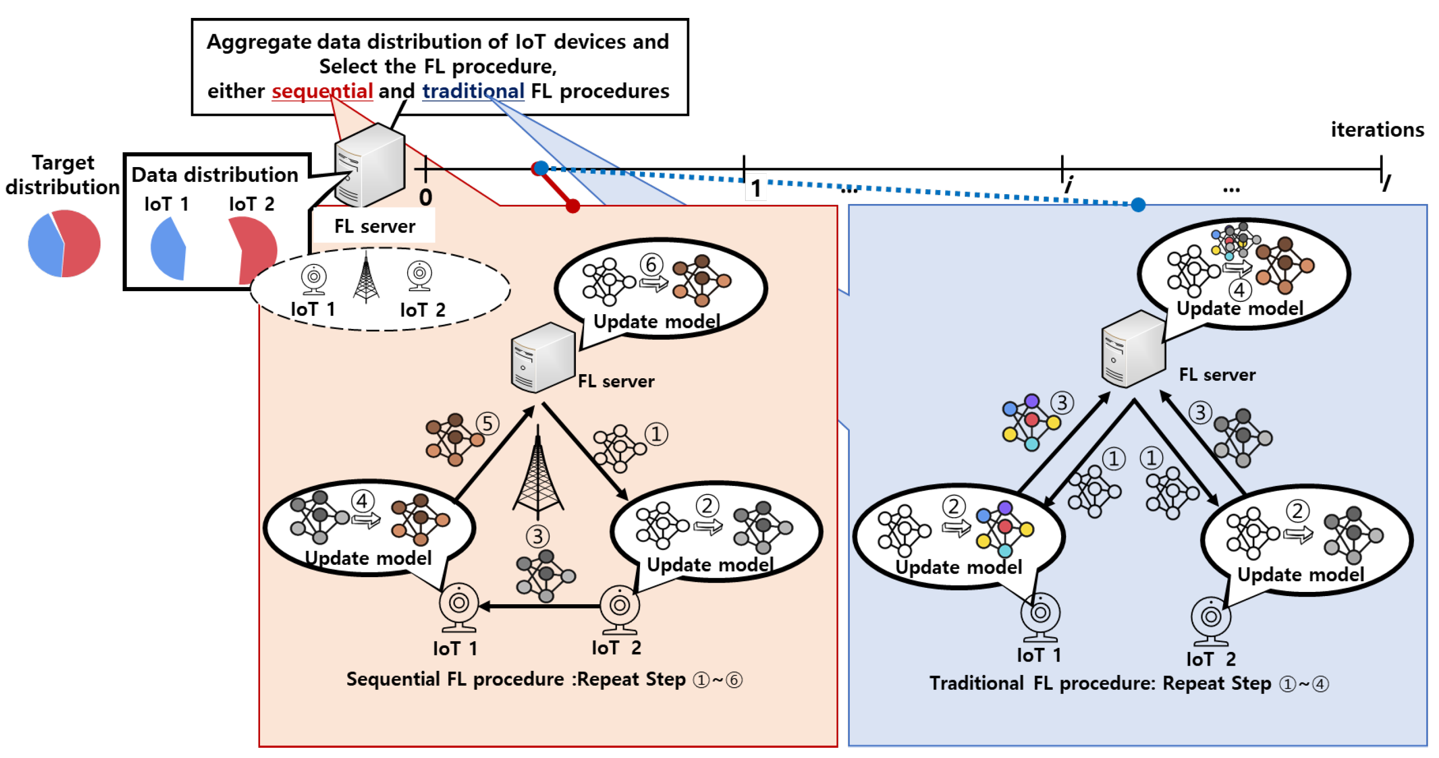
Before conducting the FL procedure, the edge server collects information about the data distribution of all IoT devices and selects one FL procedure, either the traditional or the sequential FL procedure, using the AFLS scheme that is proposed in Section 3. Specifically, when the edge server selects a sequential FL procedure, it determines the learning order of the IoT devices. Then, it notifies each IoT device of its learning order and provides information about the IoT device with the next learning order. In addition, it transmits the deep model to the IoT device assigned to the first learning order. Each IoT device trains the deep model using its private data during its assigned turn and directly transmits the updated deep model to the next IoT device in the learning order. After the last IoT device completes its training, it sends the updated model to the edge server to evaluate the trained model using test data. This process is repeated until a predefined number of iterations is completed. Since IoT devices directly transmit the deep model via D2D communication, the overall iteration time can be reduced compared to when the model is transmitted via the edge server [10].

Although the traditional FL procedure shows a relatively low convergence time compared to the sequential FL time, it also suffers from significant learning accuracy degradation in a non-IID environment. Intuitively, in a weakly non-IID environment where the data distributions of IoT devices slightly differ from the target distribution, the traditional FL procedure shows less degradation in learning accuracy. Therefore, in this case, the edge server selects the traditional FL procedure to guarantee low convergence time. Conversely, in an extremely non-IID environment, the sequential FL procedure should be selected to mitigate learning accuracy degradation. To validate this intuition, we conducted simulation studies to investigate the relationship between the degree of non-IIDness and the learning accuracy of FL procedures. We define the degree of non-IIDness, denoted as $\omega$, to quantify the difference between the average data distribution across IoT devices and the target data distribution. $\omega$ can be defined as

$$\begin{array}{c}\hfill \omega ={\displaystyle \frac{{\sum }_n{D}_{KL}\left(P_R\right|P_n)}{N}}\end{array}$$

(1)

where $D_{KL}\left(a\right|\left|b\right)$ is the Kullback–Leibler divergence (KLD) between distributions a and b [20]. A higher value of $\omega$ indicates that the data collected by IoT devices deviate more significantly from the target distribution.

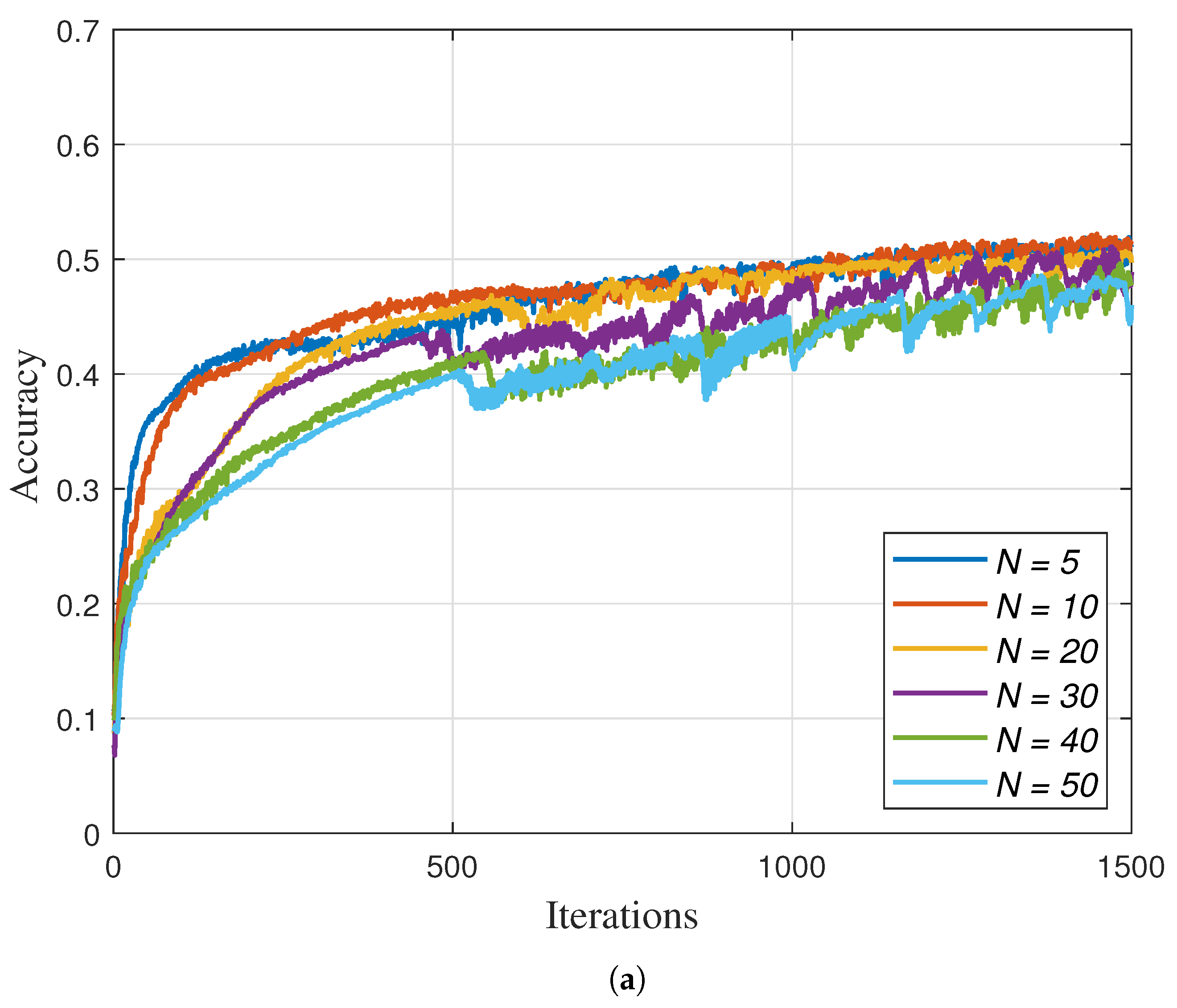
Figure 2a,b show the accuracy curves with respect to the non-IID degree $\omega$. From Figure 2a, it can be observed that when the degree of non-IIDness increases, the training accuracy of the traditional FL procedure decreases significantly. Notably, in cases of extreme non-IID (i.e., $\omega$ = 9), the accuracy is severely degraded even though the overall data distribution remains IID. In contrast, Figure 2b shows that the sequential FL procedure effectively prevents accuracy degradation, even under extreme non-IID environments. This is because the sequential FL scheme mimics a centralized training approach, where the deep model is sequentially trained using partitioned data subsets. However, the sequential FL procedure shows a significantly longer convergence time compared to the traditional FL procedures due to its inherently serialized nature. These simulation results highlight the trade-offs between learning accuracy and convergence time in traditional and sequential FL procedures under varying degrees of non-IIDness.

Based on these trade-offs, we designed an AFLS scheme that adaptively selects the FL procedure according to the non-IID degrees, $\omega$. Specifically, if the traditional FL procedure can achieve higher learning accuracy than the required threshold (i.e., when the degree of non-IIDness is lower than a certain threshold) (the threshold is assumed to be determined by the AI service provider according to the requirements of the target AI application), the traditional FL procedure should be selected to reduce the convergence time. Otherwise, the edge server needs to select the sequential FL procedure to guarantee learning accuracy.

Algorithm 1 represents the AFLS scheme. Initially, the edge server aggregates information about the data distribution of each IoT device, $P_n$, and calculates the degree of non-IIDness, $\omega$ (i.e., lines 1–2 in Algorithm 1). By comparing $\omega$ with the threshold, $\theta$, AFLS determines the appropriate FL scheme F (i.e., lines 4–7 in Algorithm 1). If F is set to SeQ, the sequential FL scheme is selected. Otherwise, if F is determined as TrA, the traditional FL scheme is chosen. Following this, the edge server initializes the AI model $A_{r,t}$ to begin the training procedure (i.e., line 8 of Algorithm 1), where r and t represent the iteration index and the learning order index within iteration r, respectively.

Based on the selected FL procedure, different operations are repeatedly performed by IoT devices and the edge server. In each iteration of the sequential FL procedure (i.e., lines 11–20 and line 27 of Algorithm 1), the edge server randomly determines the learning orders of IoT devices, where $o_t$ represents the index of IoT device assigned the tth learning order (i.e., line 11 in Algorithm 1). The edge server then informs IoT devices of information about learning orders (i.e., line 12 in Algorithm 1). After that, the edge server distributes the parameter $A_{r,0}$ to the IoT device assigned to the first learning order (i.e., line 13 in Algorithm 1). Upon receiving the parameter, the IoT device in the nth training order updates the received parameter using their data (i.e., update the parameter $P_{r,n-1}$ to the parameter $P_{r,n}$) (i.e., line 15 in Algorithm 1) and then transmits the updated parameter to the IoT device that has the next training order (i.e., line 16 in Algorithm 1). Once the IoT device that has the last training order updates the parameter, the updated parameter is transmitted to the edge server, which uses it to initialize the parameter for the next round, $A_{r+1,0}$ (i.e., lines 18–20 in Algorithm 1).

On the other hand, during a round of the traditional FL scheme (i.e., lines 21–29 in Algorithm 1), the edge server first distributes the initial parameter of round r, $A_{r,0}$ to all IoT devices (i.e., line 22 in Algorithm 1). Then, IoT devices simultaneously update the initial parameter with their data and upload its updated parameter $A_{r,n}$ to the edge server (i.e., lines 23–26 in Algorithm 1). Once the edge server receives the updated parameters from all IoT devices, it aggregates them to create the initial parameter for the next round, $A_{r+1,0}$ (i.e., line 27 in Algorithm 1). When the edge server updates the parameter at the end of round r, regardless of the determined FL procedure, it evaluates the accuracy of the AI model using the parameter $A_{r+1,0}$ (i.e., line 29 in Algorithm 1). Note that the complexity of AFLS is given by $\mathcal{O}\left(N\right)$, where $\mathcal{O}\left(\right)$ denotes the big O notation. This complexity arises from aggregating the data distribution and computing the overall non-IID degree of IoT devices (i.e., lines 1 and 2 in Algorithm 1). Since the complexity is linear in the number of devices, AFLS is lightweight and can be efficiently implemented in practical systems.

Algorithm 1 AFLS scheme

1: Aggregate the data distribution of IoT devices $P_n,\forall n$  2: Calculates the overall non-IID degree of IoT devices, $\omega$  3: if$\omega \ge \theta$then  4:    Selects the sequential FL procedure $F=\mathrm{SeQ}$  5: else  6:    Selects the traditional FL procedure $F=\mathrm{TrA}$  7: end if  8: Initialize the AI model with the parameter $A_{0,0}$  9: for$r\in \mathbf{R}$do 10:    if $F=\mathrm{SeQ}$ then 11:      Randomly determine the learning order vector $\mathbf{o}=[o_1,o_2,\dots ,o_N]$ 12:      Notify learning order information to all IoT devices 13:      Transmits parameter of AI model $A_{r,0}$ to $o_1$ IoT device having first learning order 14:      for $n^{\prime }$ in $[1,2,3,\dots ,N-1]$ do 15:         Update $A_{r,n^{\prime }-1}$ to $A_{r,n^{\prime }}$ by $o_{n^{\prime }}$ IoT device 16:         Transmit $A_{r,n^{\prime }}$ to $o_{n^{\prime }+1}$ IoT device from $o_{n^{\prime }}$ IoT device 17:      end for 18:      Update $A_{r,N-1}$ to $A_{r,N}$ by $o_N$ IoT device 19:      Transmit $A_{r,N}$ to the FL server from $o_N$ IoT device 20:      Update the received parameter by $A_{r+1,0}=A_{r,N}$ at the edge server 21:    else 22:      Transmits $A_{r,0}$ to all IoT device 23:      for all n do parallel do 24:         Update $A_{r,0}$ to $A_{r,n}$ by IoT device n 25:         Transmit the $A_{r,n}$ to the edge server from IoT device n 26:      end for 27:      Updates $A_{r,0}$ to $A_{r+1,0}$ by the received parameters $P_{A,n},\forall n$ 28:    end if 29:    Evaluate the accuracy of the AI model $A_{r+1,0}$ 30: end for

4. Evaluation Results

To evaluate the performance of the AFLS scheme, we compared AFLS with three schemes: (1) FedTrA [2,16], where the traditional FL procedure is conducted using all devices (note that FedTrA represents the traditional FL procedure, including recent variants such as the one proposed in [16]); (2) FedSeQ [10,19], where the sequential learning procedure without D2D communication is conducted; and (3) FedSeQ-D2D, where the sequential learning procedure with D2D communication is conducted. (In this paper, we selected baseline schemes that share the same underlying principle as AFLS to fairly evaluate its decision-making between two fundamental FL procedures (i.e., traditional and sequential FL). However, in future work, we will compare AFLS with more advanced FL schemes to provide a broader understanding of its performance).

We exploit CIFAR-10 [21], which is a classic object classification dataset consisting of $50,000$ training data and $10,000$ testing images with 10 object classes. This dataset has been used commonly in FL studies [2,15]. The deep classification model is used by the CNN model to classify CIFAR-10 data. We consider 10 IoT devices (note that we conducted simulations with varying numbers of IoT devices, ranging from 5 to 50, and we observed that the performance trends remained consistent regardless of the number of participating devices), and each device has only data from K classes among 10 classes. Moreover, we set the communication time and computation time of devices as uniform values. The device has the same amount of data, whereas each device randomly K classes data among 10 classes. For instance, if we set K as 2 to consider the extreme non-IID case, $\omega$ is 9. The required accuracy was set to $0.6$.

4.1. Effect on N

Figure 3a,b show the learning accuracy of the traditional and sequential FL procedures, respectively, as a function of the number of participating IoT devices, N. In this simulation, we set K to 2 to simulate an extreme non-IID scenario ($\omega =9$). In this case, the traditional FL procedure cannot achieve the required accuracy due to the extremely non-IID data of IoT devices. On the other hand, in the same environment, the sequential FL procedure achieve the required accuracy, and thus, AFLS selected the sequential FL procedure.

Interestingly, Figure 3 shows that the traditional FL procedure converges more slowly as N increases. In contrast, the convergence speed of the sequential FL procedure is faster with a larger N. This is because, in the traditional FL procedure, as N increases, each IoT device holds a smaller amount of data, which makes it difficult to sufficiently train the global model during each round. On the other hand, in the sequential FL procedure, even when each device holds only a small amount of data, the random ordering of devices across iterations introduces diverse data sequences, which enhances the training efficiency of the global model.

In addition, Figure 4a,b show the achieved accuracy and convergence time as a function of the number of IoT devices, N. AFLS, FedSeQ, and ${\mathrm{FedSeQ}}_{\mathrm{D}2\mathrm{D}}$ consistently achieve higher accuracy than the required threshold (i.e., 0.6), regardless of N, whereas FedTrA fails to meet the required accuracy at any device count. This is because the diversity of model parameters trained in the traditional FL procedure, resulting from non-IID data, hinders the convergence of the global model. Due to this reason, AFLS selects ${\mathrm{FedSeQ}}_{\mathrm{D}2\mathrm{D}}$ to mitigate accuracy degradation while reducing convergence time.

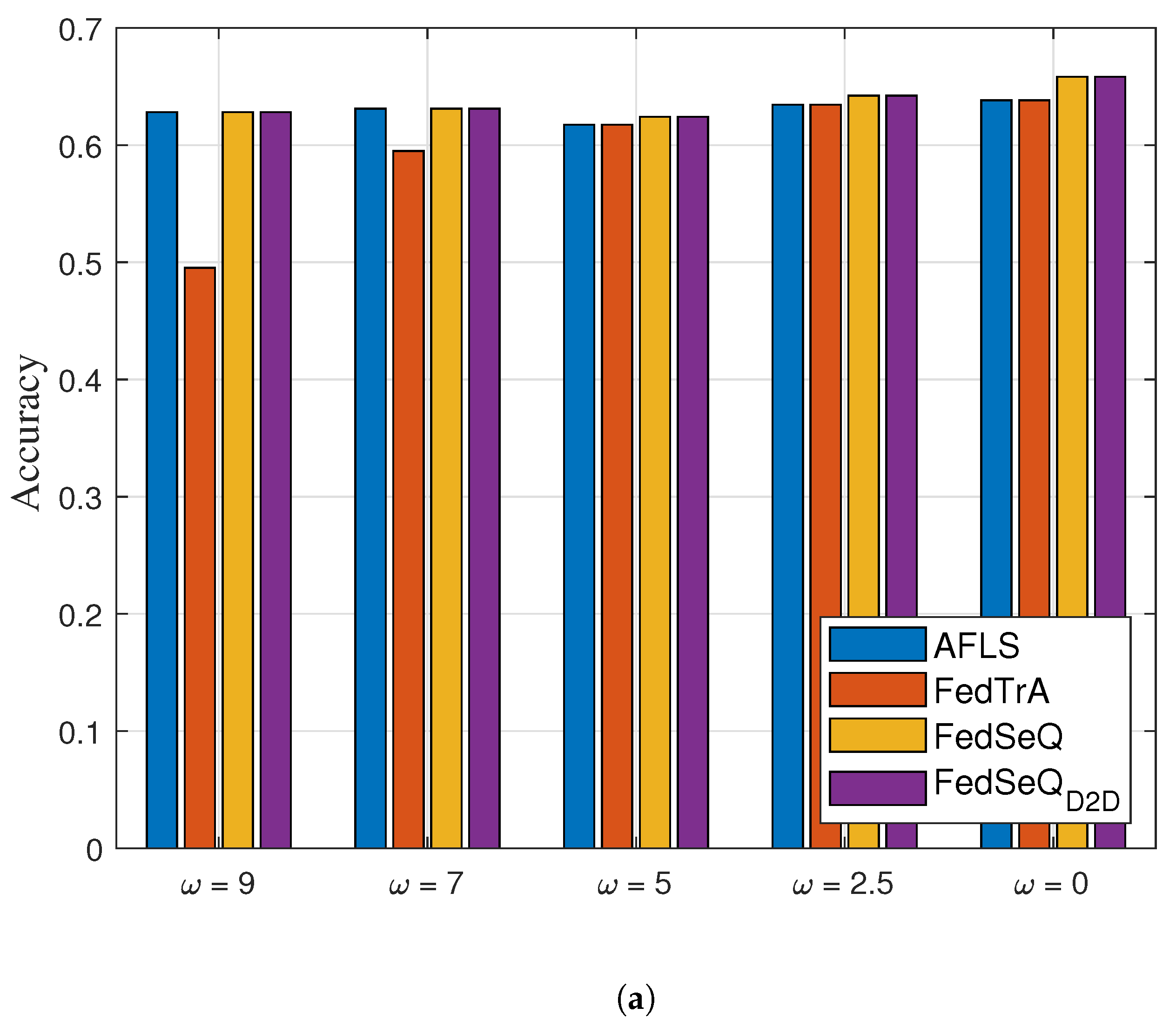
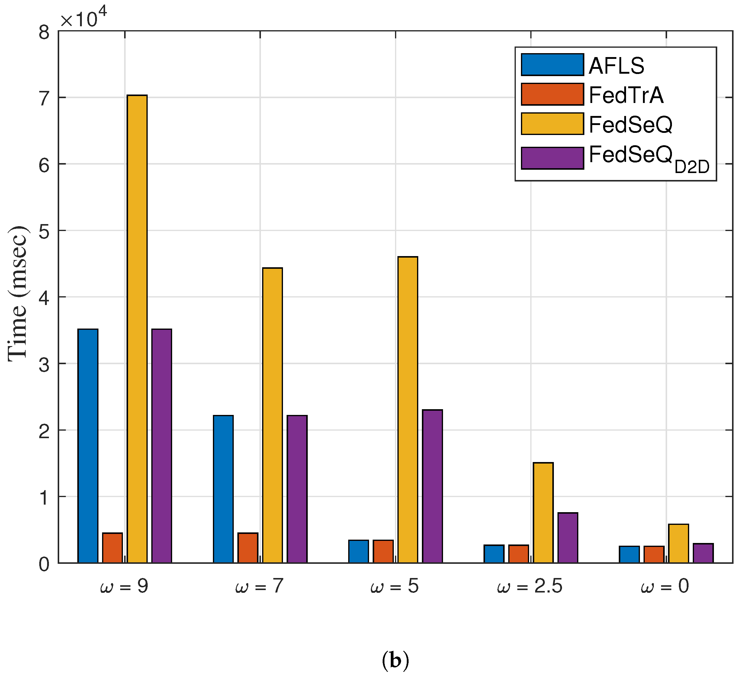
4.2. Effect on $\omega$

Figure 5a,b show the achieved accuracy and the convergence time as a function of the degree of non-IIDness, $\omega$. As illustrated in Figure 5a, AFLS, FedTrA, and ${\mathrm{FedSeQ}}_{\mathrm{D}2\mathrm{D}}$ consistently achieve accuracy above the required threshold of 0.6, regardless of the non-IID degree $\omega$. In contrast, FedTrA fails to satisfy the accuracy requirement under highly non-IID conditions (i.e., $\omega =9$). This is because the parameter divergence induced by non-IID data in traditional FL schemes hinders the convergence of the global model.

Although FedSeQ and ${\mathrm{FedSeQ}}_{\mathrm{D}2\mathrm{D}}$ can meet the required accuracy, these schemes incur longer convergence times due to their inherently sequential training process. In particular, FedSeQ exhibits a longer convergence time than ${\mathrm{FedSeQ}}_{\mathrm{D}2\mathrm{D}}$, as model updates must be relayed indirectly through the edge server. In contrast, AFLS achieves shorter convergence times than both FedSeQ variants when the non-IID degree is moderately high (i.e., $\omega <9$) by adaptively selecting a more efficient FL mode. It is worth noting that FedTrA consistently exhibits the shortest convergence time across all cases. However, it suffers from severe accuracy degradation under non-IID conditions.

5. Conclusions

In this paper, we proposed an adaptive FL procedure selection scheme (AFLS) that selects an appropriate FL scheme, either the traditional or the sequential FL procedures, based on the degree of non-IID among IoT devices to achieve both the required learning accuracy and low convergence time. To further reduce the convergence time of the sequential FL procedure, we also introduced a device-to-device (D2D)-based sequential FL procedure. If the data characteristics of IoT devices change over time, i.e., the degree of non-IIDness dynamically varies, the initially selected FL procedure may no longer remain optimal. For future work, we plan to design a novel FL scheme in which multiple sequential FL procedures are simultaneously executed by the edge server, aiming to enhance parallelism to reduce the convergence time while still benefiting from robustness regarding non-IID data offered by sequential learning.