Fuzzy-Based Composite Nonlinear Feedback Cruise Control for Heavy-Haul Trains

Abstract

To improve the transient performance of speed tracking control while ensuring stability and considering actuator constraints in heavy-haul train systems, this paper proposes a novel cruise control method based on a nonparallel distributed compensation (non-PDC) fuzzy-based composite nonlinear feedback (CNF) technique. First, a low-dimensional nonlinear multi-particle error dynamics model is established based on the fencing concept, simplifying the model significantly. To facilitate controller design, a Takagi–Sugeno (T-S) fuzzy model is derived from the nonlinear model. Subsequently, sufficient conditions for the non-PDC fuzzy-based CNF controller are provided in terms of linear matrix inequalities (LMIs), with the controller design addressing asymmetric constraints on control inputs due to differing maximums of traction and braking forces. Simulations based on MATLAB/Simulink are conducted under different maneuvers to validate the effectiveness and superiority of the proposed method. The simulation results demonstrate a notable enhancement in transient performance (over 22.3% improvement in settling time) and steady-state cruise control performance for heavy-haul trains using the proposed strategy.

1. Introduction

Owing to their advantages in transportation capability, energy consumption, and commercial cost, heavy-haul railways have attracted increasing attention. It is estimated that over 60% of coal transportation in China is carried out via heavy-haul railways [1]. To meet the growing demand for coal transportation, the loading capacity of heavy-haul trains has increased to 20,000 tons, posing great challenges to train operation. To this end, it is necessary and imminent to develop automatic control strategies for heavy-haul trains to reduce driver workload and improve transportation efficiency.

Researchers have proposed several advanced control methods for speed regulation and energy consumption optimization in heavy-haul trains. To depict the dynamic behavior of heavy-haul trains, early research employed a single-particle model that ignored interactions between each car and considered the whole train as a single mass point. This approach remains common in curve optimization problems [2,3,4]. While the single-particle model is concise and simplifies controller design, it neglects in-train forces that play a crucial role in ensuring operational safety. Therefore, in-train forces should be taken into account when modeling.

Given the above analysis, Zhuan et al. [5] proposed a multi-particle model that portrays a train as a series of individual cars connected by couplers. The corresponding control strategies have been developed fruitfully. In [5], based on the Lagrange multiplier method, authors proposed an open-loop scheduling considering the input constraint to minimize the in-train forces. Moreover, an optimal control strategy that can adapt to various train configurations was explored in [6]. In [7], a distributed cooperative control method considering varying communication delays was proposed to track the desired speed and minimize in-train forces. Given the ability of model predictive control (MPC) methods to address both input and state constraints, authors of [8,9,10,11] introduced it for heavy-haul train control. Rather than minimize the in-train force in the research mentioned above, the MPC can limit the in-train force within a definite range, i.e., a hard constraint of the in-train force, which can ensure operation safety essentially. Ref. [9] utilized a brake penalty strategy to save energy and reduce in-train forces without sacrificing the speed tracking performance. Additionally, authors of [10] incorporated coupler damping effects into the cost function, successfully alleviating the cyclic vibrations of the coupler. Considering the packet dropouts in communication, ref. [11] presented a robust MPC method that solved the corresponding controller by deriving a set of linear matrix inequalities (LIMs). Although the MPC method can tackle the state and input constraints problem simultaneously, its significant online computational demand remains a notable drawback, especially for such a fast-changing electromechanical system. To save energy, refs. [12,13] designed a periodic intermittent controller and a state-dependent intermittent control, respectively, accounting for parameter uncertainties and input constraints. Simulation results showed a notable improvement in control efficiency with only a modest impact on speed tracking performance. Nevertheless, the resistance force caused by the slope was not considered in these two papers.

The longitudinal dynamics model of the heavy–haul train is inherently nonlinear due to the nonlinearity of the basic running resistance, braking forces, in-train forces, etc. However, the control methods mentioned above are all based on a linear multi-particle model obtained through linearization, which may result in a model mismatch, leading to a poor control effect to some degree. To solve this problem, several nonlinear control strategies were explored. In [14], an output feedback tracking controller considering input constraints was formulated and applied to speed regulation for heavy-haul trains. The simulation results demonstrated its simplicity, cost-effectiveness, and implementation convenience. Instead of tracking a desired speed, the trajectory tracking problem for heavy-haul trains was explored in [15]. A nonlinear consensus control method was designed, which innovatively treats the wagons’ braking forces as passive frictions rather than as active control efforts. In [16], a novel dynamic auxiliary compensator was designed to compensate for saturation error. Subsequently, an anti-saturation sliding mode control algorithm was introduced to ensure stability and enhance performance. An adaptive nonsingular terminal sliding mode control was employed in [17], considering the control command delay. Compared with linear controllers, nonlinear controllers are more sophisticated. With the development of control techniques, intelligent controls, such as the genetic algorithm [18], machine learning [19], and deep-Q-network algorithm [20], have been adopted in heavy-haul train operations. These methods require large amounts of data and high-performance hardware support, making them unsuitable for online applications.

To simplify the modeling of nonlinear systems, the Takagi–Sugeno (T-S) modeling technique was proposed in 1985 [21], by which the nonlinear system can be approximated to any degree of accuracy by blending a series of linear models through fuzzy IF-THEN rules. Therefore, well-studied linear control theories can be effectively applied to the T-S model, facilitating the stabilization of nonlinear systems. Owing to this advantage, T-S model-based control methods have widespread application in nonlinear systems, including speed tracking control for high-speed trains [22,23].

In practical heavy-haul train operational scenarios, drivers pursue a small steady-state error and a short settling time without overshooting in speed tracking to enhance safety. To improve the transient performance, a new control technique called composite nonlinear feedback (CNF) was proposed in 2003 [24]. The CNF controller consists of linear and nonlinear parts, where the linear part stabilizes the system while the nonlinear part enhances the transient performance. Moreover, the actuator saturation can be considered simultaneously. However, one drawback of CNF is its limitation to linear systems, which restricts its application in heavy-haul trains.

To compensate for the shortcomings, researchers have focused on extending the CNF concept to nonlinear systems, which has become a research hotspot. Based on the above analysis, a promising idea that can develop a novel algorithm combining the advantages of these two techniques arises to improve the dynamic response performance of nonlinear systems. This work was initially proposed by Ebrahimi et al. [25] and further developed by Hu et al. [26]. Both control methods utilized the concept of parallel distribution compensation (PDC) to design the T-S fuzzy controller, which, has a concise expression but low flexibility. In addition, the fuzzy-model-based CNF control algorithms presented in these papers are limited to single-input, single-output (SISO) systems with symmetric input constraints, making them unsuitable for direct application to multi-input, multi-output (MIMO) systems, such as heavy-haul trains.

Since cruise mode dominates the overall operational schedule—especially for heavy-haul trains with large station spacing—employing an efficient cruise control strategy can enhance operational performance. Inspired by the above analysis, this paper focuses on designing a cruise controller with a small calculation burden for heavy-haul trains considering actuator saturation, transient performance enhancement, high flexibility, and less conservatism. To this end, a non-PDC fuzzy-based CNF cruise control approach is proposed. The main contributions of this paper are summarized as follows:

(1)

A novel fuzzy CNF control strategy is proposed for the heavy-haul train cruise control system, ensuring system robustness while improving transient performance.

(2)

A MIMO T-S fuzzy model is developed for heavy-haul trains, incorporating slope resistance force. This mitigates model mismatch and enhances the accuracy of the dynamic model.

(3)

By taking into account the asymmetric traction/braking force constraints, a non-PDC controller is designed as the linear part of the CNF controller. This approach improves design flexibility and reduces conservativeness compared to existing PDC-based CNF controllers. Additionally, the proposed controller can be directly applied to MIMO systems represented by T-S fuzzy models, broadening the scope of current methodologies that predominantly address SISO systems.

The remainder of the paper is organized as follows. In Section 2, the multi-particle error dynamics model for the heavy-haul train is established and transformed as a T-S model. Section 3 discusses the design of the non-PDC fuzzy-based CNF controller. Simulation results are presented in Section 4, and conclusions are drawn in Section 5.

2. Problem Statement

2.1. The Dynamics Model of Heavy-Haul Trains

Figure 1 shows the longitudinal motion of the heavy-haul train. It is assumed that the heavy-haul train consists of $l_w$ wagons and $l_l$ locomotives. The longitudinal dynamics of heavy-haul trains can be depicted as

$$m_q{\dot{v}}_q=F_q-F_{Rg,q}-F_{Rs,q}-F_{Rr,q}+F_{in,q-1}-F_{in,q},\mathrm{for}q=1,\dots ,l,$$

(1)

where $m_q$ is the car mass, $v_q$ represents the speed, $F_q$ denotes the traction/braking efforts, $F_{in,q}$ implies the in-train force between the qth and $(q+1)$th car, $F_{Rg,q}$ denotes the general running resistance, $F_{Rs,q}$ and $F_{Rc,q}$ are resistances caused by the track slope and curvature on which the qth car is running. l implies the number of cars and $l=l_l+l_w$. $F_{Rg,q}$, $F_{Rs,q}$, and $F_{Rc,q}$ can be represented as the following empirical formulas [27]

$$\begin{array}{cc}\hfill F_{Rg,q}& =m_{q}g\left(a_0+a_1{v}_q+a_2{v}_q^2\right),\hfill \end{array}$$

(2)

$$\begin{array}{cc}\hfill F_{Rs,q}& =m_{q}gsin{\theta }_q\approx m_{q}g{\theta }_q,\hfill \end{array}$$

(3)

$$\begin{array}{cc}\hfill F_{Rc,q}& =m_{q}g{\displaystyle \frac{600}{R_q}},\hfill \end{array}$$

(4)

where g is the acceleration of gravity, $a_0$, $a_1$, and $a_2$ are coefficients that relate to train properties, ${\theta }_q$ represents the slope angle, and $R_q$ denotes the track curve radius. By referring to [6], the coupler system can be regarded as a spring with a damper. With the damping effect ignored, the in-train force $F_{in,q}$ can be simplified as

$$F_{in,q}=k_q{x}_{in,q},\mathrm{for}q=1,\dots ,l-1,$$

(5)

where $k_q$ is the stiffness coefficient, and $x_{in,q}$ is the relative displacement of the qth and $(q+1)$th car.

To analyze the in-train force, the relative displacement is introduced. Then, the following multi-particle model is used to describe the longitudinal dynamics of heavy-haul trains.

$$\left\{\begin{array}{c}{m}_q{\dot{v}}_q=F_q-F_{Rg,q}-F_{Rc,q}-F_{Rr,q}+F_{in,q-1}-F_{in,q},\mathrm{for}q=1,\dots ,l\hfill \\ {\dot{x}}_{in,q}=v_q-v_{q+1}, \mathrm{for}q=1,\dots ,l-1\hfill \end{array}\right.,$$

(6)

where $F_{in,0}=0$.

By substituting (2)–(5) into (6) and assuming $k_1=k_2=\dots =k_q=k$, we can obtain the following simplified model

$$\left\{\begin{array}{cc}{m}_q{\dot{v}}_q=F_q-m_{q}g\left(a_0+a_1{v}_q+a_2{v}_q^2+{\displaystyle \frac{600}{R_q}}+{\theta }_q\right)+k\left(x_{in,q-1}-x_{in,q}\right)\hfill & \\ \mathrm{for}q=1,\dots ,l\hfill \\ {\dot{x}}_{in,q}=v_q-v_{q+1},\mathrm{for}q=1,\dots ,l-1\hfill \end{array}\right..$$

(7)

Although the brake force contains the rheostatic and air brake force, in normal conditions, such as the cruise maneuver, the rheostatic brake force is enough to sustain the heavy-haul trains’ speed. In this paper, a cruise control strategy will be explored only considering rheostatic brake force. It should be noted that both the traction and rheostatic brake efforts are only assembled on locomotives. To reduce the model dimension, the fencing concept that uses one control signal to control all the cars within the same group is utilized [6]. Accordingly, the heavy-haul train depicted by (7) can be divided into $l_l$ groups. Furthermore, we assume that the aerodynamic resistance acts only on the front group and the rolling resistance affects each group. Then, the dynamic Equation (7) can be transformed into

$$\left\{\begin{array}{c}{M}_1{\dot{v}}_1=F_1-M_{1}g\left(a_0+a_1{v}_1\right)-\left({\displaystyle \sum _{p=1}^{l_l}}{M}_{p}g\right)a_2{v}_1^2+k{x}_{in,1}-M_{1}g\left({\theta }_1+{\displaystyle \frac{600}{R_1}}\right)\hfill \\ M_p{\dot{v}}_p=F_p-M_{p}g\left(a_0+a_1{v}_p\right)+k\left(x_{in,p-1}-x_{in,p}\right)-M_{p}g{\theta }_p-M_{p}g{\displaystyle \frac{600}{R_p}},\hfill & \\ \mathrm{for}p=2,\dots ,l_l-1\hfill \\ M_{l_l}{\dot{v}}_{l_l}=F_{l_l}-M_{l_l}g\left(a_0+a_1{v}_{l_l}\right)+k{x}_{in,l_l-1}-M_{l_l}g{\theta }_{l_l}-M_{l_l}g{\displaystyle \frac{600}{R_{l_l}}}\hfill & \\ {\dot{x}}_{in,p}=v_p-v_{p+1},\mathrm{for}p=1,\dots ,l_l-1\hfill \end{array}\right.,$$

(8)

where $M_p$, $F_p$ and $v_p$ are the mass, traction/braking force and speed of the p th group, $R_p$ and ${\theta }_p$ are track radius and slope.

Since the speeds of heavy-haul trains and displacements of couplers are constant in cruise mode, this operation mode can be regarded as an equilibrium state. For simplicity, we define the target speed of each group as $v_r$ and the desired relative displacement $x_{in,r}=0$ at the equilibrium point in this paper. Based on these assumptions, we can calculate the following steady-state control efforts using (8).

$$\left\{\begin{array}{c}{u}_{eq,1}=M_{1}g\left(a_0+a_1{v}_r\right)+\left(\sum _{p=1}^{l_l}{M}_{p}g\right)\ast a_2{v}_r^2+M_{1}g{\theta }_1+M_{1}g{\displaystyle \frac{600}{R_1}}\hfill \\ u_{eq,p}=M_{p}g\left(a_0+a_1{v}_r\right)+M_{p}g{\theta }_p+M_{p}g{\displaystyle \frac{600}{R_p}},\mathrm{for}p=2,3,\dots ,l_l\hfill \end{array}\right..$$

(9)

Define $e_{in,p}=x_{in,p}-x_{in,r}$, $e_{v,p}=v_p-v_r$, $u_{e,p}=F_p-u_{eq,p}\left(p=1,\dots ,l_l\right)$, and choose $x={\left[e_{v,1},\dots ,e_{v,l_l},e_{in,1},\dots ,e_{in,l_{l-1}}\right]}^T$ as state variables, $u={\left[u_{e,1},\dots ,u_{e,l_l}\right]}^T$ as control inputs and $y={\left[e_{v,1},e_{v,2},\dots ,e_{v,l_l}\right]}^T$ as output signals. Subsequently, the error equation can be established as follows

$$\left\{\begin{array}{c}\dot{x}=A\left(x\right)x+Bu\hfill \\ y=Cx\hfill \end{array}\right.,$$

(10)

where $A\left(x\right)={\left[\begin{array}{cc}{\Gamma }_1& {\Gamma }_2\\ {\Gamma }_3& 0\end{array}\right]}_{(2l_1-1)\times (2l_1-1)}$, $a_{11}=-g\left(a_1+{\displaystyle \frac{\left({\sum }_{p=1}^{l_l}{M}_p\right)\ast a_2(e_{v,1}+2v_r)}{M_1}}\right)$,

${\Gamma }_1=\left[\begin{array}{ccccc}{a}_{11}& 0& 0& \dots & 0\\ 0& -g{a}_1& 0& \dots & 0\\ 0& 0& -g{a}_1& \dots & 0\\ ⋮& \ddots & \ddots & \ddots & ⋮\\ 0& 0& 0& \dots & -g{a}_1\end{array}\right]$, ${\Gamma }_2=\left[\begin{array}{cccc}-{\displaystyle \frac{k}{M_1}}& 0& \dots & 0\\ {\displaystyle \frac{k}{M_2}}& -{\displaystyle \frac{k}{M_2}}& \dots & 0\\ 0& {\displaystyle \frac{k}{M_3}}& \dots & 0\\ ⋮& ⋮& \ddots & ⋮\\ 0& 0& \dots & -{\displaystyle \frac{k}{M_p}}\end{array}\right]$,

${\Gamma }_3=\left[\begin{array}{ccccc}1& -1& 0& \dots & 0\\ 0& 1& -1& \dots & 0\\ ⋮& \ddots & \ddots & \ddots & ⋮\\ 0& \dots & 0& 1& -1\end{array}\right]$, $B=\left[\begin{array}{c}diag\left({\displaystyle \frac{1}{M_1}},\dots ,{\displaystyle \frac{1}{M_{l_l}}}\right)\\ 0_{l_l\times (l_l-1)}\end{array}\right]$, $C=\left[I_{l_l\times l_l},0_{l_l\times (l_l-1)}\right]$. Since the state variable $e_{v,1}$ is contained in matrix $A\left(x\right)$, the established system (10) is a nonlinear MIMO system essentially.

The practical traction and braking forces have limitations resulting from the characteristics of actuators. Thus, the following input constraints should be taken into account in modeling and controller design.

$$\begin{array}{c}\hfill -F_{min,p}\le F_p\le F_{max,p}\end{array},$$

(11)

where $F_{max,p}$ and $F_{min,p}$ are positive scalars representing the maximum traction and braking forces of the pth locomotive, respectively. Since $F_{max,p}$ and $F_{min,p}$ are usually different, the input constraint is asymmetric. To convert the asymmetric saturation system into a symmetric one, (11) can be rewritten as

$$-u_{max,p}\le u_{e,p}-\left({\displaystyle \frac{F_{max,p}-F_{min,p}}{2}}-u_{eq,p}\right)\le u_{max,p},$$

(12)

where $u_{max,p}={\displaystyle \frac{F_{max,p}+F_{min,p}}{2}}$. By defining a new input ${\overline{u}}_p=u_{e,p}-\left({\displaystyle \frac{F_{max,p}-F_{min,p}}{2}}-u_{eq,p}\right)$, we obtain a symmetric input constraint as follows:

$$sat\left({\overline{u}}_p\right)=sgn\left({\overline{u}}_p\right)·min\{u_{max,p},|{\overline{u}}_p\left|\right\}.$$

(13)

Subsequently, (10) is transformed as

$$\left\{\begin{array}{c}\dot{x}=A\left(x\right)x+Bsat\left(\overline{u}\right)+B_{w}w\hfill \\ y=Cx\hfill \end{array}\right.,$$

(14)

where $\overline{u}=\left[\begin{array}{c}{\overline{u}}_1\\ ⋮\\ {\overline{u}}_{l_l}\end{array}\right]$, $B_w=B$, $w=\left[\begin{array}{c}{\displaystyle \frac{F_{max,1}-F_{min,1}}{2}}-u_{eq,1}\\ {\displaystyle \frac{F_{max,2}-F_{min,2}}{2}}-u_{eq,2}\\ ⋮\\ {\displaystyle \frac{F_{max,l_l}-F_{min,l_l}}{2}}-u_{eq,l_l}\end{array}\right]$.

2.2. The T-S Model of Heavy-Haul Trains

As a universal approximator for nonlinear systems, the T-S fuzzy model is introduced in this paper to facilitate the controller design. Suppose that $e_{v,1}$ varies from $e_{v,min}$ to $e_{v,max}$. Owing to the “sector nonlinearity” approach, $e_{v,1}$ can be represented as

$$e_{v,1}=h_1\left(\xi \right)e_{v,min}+h_2\left(\xi \right)e_{v,max},$$

(15)

where $\xi$ is the defined premise variable and $\xi =e_{v,1}$, $h_1\left(\xi \right)$ and $h_2\left(\xi \right)$ are membership functions, and $h_1\left(\xi \right)={\displaystyle \frac{{\xi }_{max}-\xi }{{\xi }_{max}-{\xi }_{min}}}$, $h_2\left(\xi \right)={\displaystyle \frac{\xi -{\xi }_{min}}{{\xi }_{max}-{\xi }_{min}}}$, ${\xi }_{max}=e_{v,max}$, ${\xi }_{min}=e_{v,min}$. Then, the T-S model for heavy-haul trains can be described by the following fuzzy IF-THEN rules

$$\left\{\begin{array}{c}\mathrm{IF}\xi \mathrm{is}{h}_1,\mathrm{THEN}\dot{x}=A_{1}x+Bsat\left(\overline{u}\right)+B_{w}w\hfill \\ \mathrm{IF}\xi \mathrm{is}{h}_2,\mathrm{THEN}\dot{x}=A_{2}x+Bsat\left(\overline{u}\right)+B_{w}w\hfill \end{array}\right.,$$

(16)

where $A_1$ and $A_2$ are obtained from matrix $A\left(x\right)$ in (14) by replacing $e_{v,1}$ with ${\xi }_{min}$ and ${\xi }_{max}$, respectively. Therefore, the T-S model can be represented as

$$\left\{\begin{array}{c}\dot{x}=\sum _{i=1}^2{h}_i\left(\xi \right)A_{i}x+Bsat\left(\overline{u}\right)+B_{w}w\hfill \\ y=Cx\hfill \end{array}\right..$$

(17)

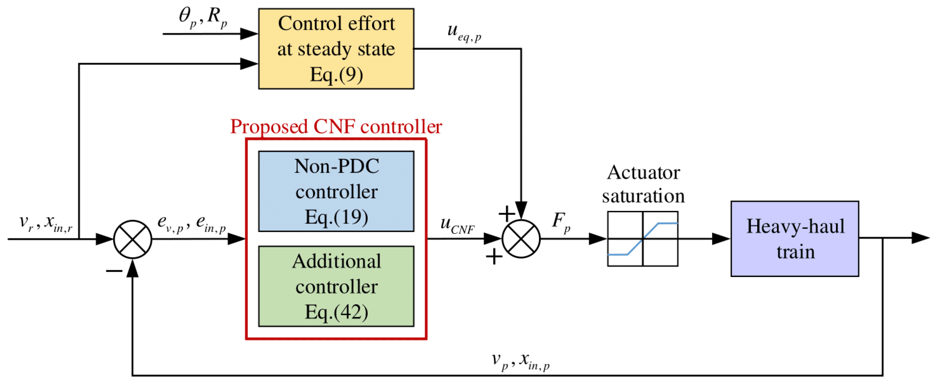
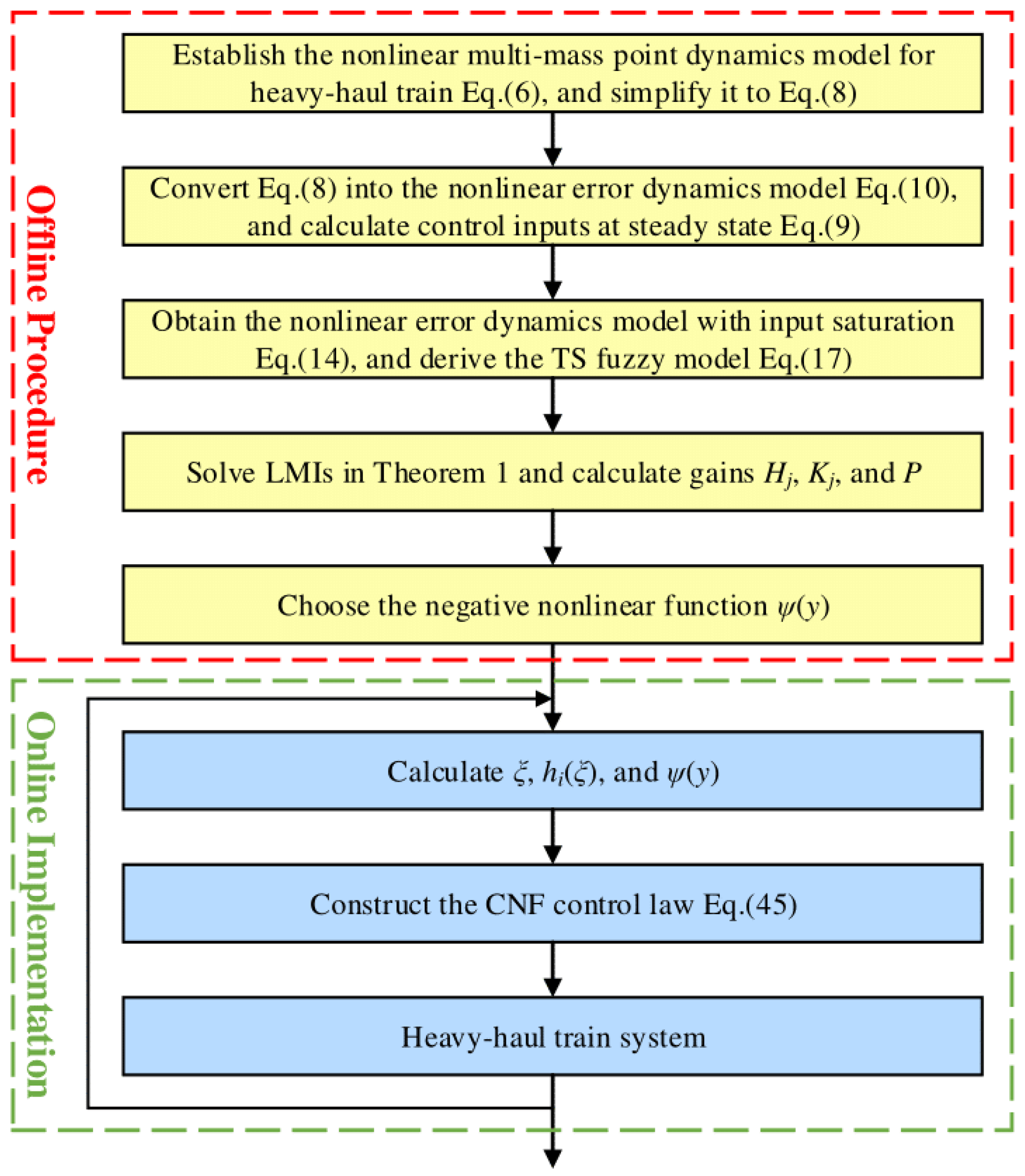
3. Non-PDC Fuzzy-Based CNF Controller Design

To achieve the cruise control goal of heavy-haul trains, a novel non-PDC fuzzy-based CNF controller is developed in this section. The structure of the proposed CNF controller is shown in Figure 2. The proposed controller comprises a non-PDC controller for closed-loop stability and an additional controller to enhance the transient performance. The overall controller $u_{CNF}$ can be expressed as

$$u_{CNF}=u_{non-PDC}+u_{add},$$

(18)

where $u_{non-PDC}$ represents the non-PDC controller, and $u_{add}$ denotes the additional controller. In addition, it should be noted that $\overline{u}=u_{CNF}$. Therefore, according to the definition of the control system model, the traction/braking efforts of each group $F_p=u_{CNF}^{\left(p\right)}+u_{eq,p}$, where $u_{CNF}^{\left(p\right)}$ represents the pth row of the vector $u_{CNF}$.

3.1. Design of Non-PDC Controller

To ensure the stability of the closed system, a non-PDC controller is constructed as follows

$$u_{non-PDC}=\left(\sum _{i=1}^2{h}_i\left(\xi \right)K_i\right){\left(\sum _{i=1}^2{h}_i\left(\xi \right)H_i\right)}^{-1}x=K_n{H}_n^{-1}x,$$

(19)

where $H_i=H_i^T>0$, $H_n={\sum }_{i=1}^2{h}_i\left(\xi \right)H_i$, $K_n={\sum }_{i=1}^2{h}_i\left(\xi \right)K_i$. To develop the stabilizing controller, the following lemmas have been employed:

Lemma 1

([28]). Consider the actuator saturation issues defined by (13), as long as $|{\overline{u}}_p|<u_{max,p}/{\epsilon }_p$, where ${\epsilon }_p$ is an arbitrary constant satisfying ${\epsilon }_p\in (0,1)$, the following inequality can be obtained

$${\left(sat\left({\overline{u}}_p\right)-{\displaystyle \frac{1+{\epsilon }_p}{2}}{\overline{u}}_p\right)}^T\left(sat\left({\overline{u}}_p\right)-{\displaystyle \frac{1+{\epsilon }_p}{2}}{\overline{u}}_p\right)\le {\left({\displaystyle \frac{1-{\epsilon }_p}{2}}\right)}^2{\overline{u}}_p^T{\overline{u}}_p.$$

(20)

Lemma 2

([29]). For an arbitrary parameter ${\Xi }_{ij}$, the inequality ${\sum }_{i=1}^r{\sum }_{j=1}^r{h}_i\left(\xi \right)h_j\left(\xi \right){\Xi }_{ij}<0$ is satisfied if

$$\left\{\begin{array}{c}{\Xi }_{ii}<0\hfill \\ {\displaystyle \frac{2}{r-1}}{\Xi }_{ii}+{\Xi }_{ij}+{\Xi }_{jj}<0\hfill \end{array}\right.,\mathrm{for}1\le i\ne j\le r,$$

(21)

where r is the number of fuzzy rules.

Lemma 3

((Finsler’s Lemma) [30]). Let $x\in {\mathbb{R}}^n$, $\mathbb{Q}={\mathbb{Q}}^T\in {\mathbb{R}}^n$ and $X\in {\mathbb{R}}^{s\times n}$ such that $rank\left(X\right)<n$. The following statements are equivalent:

$\begin{array}{cccc}& \left(1\right)\hfill & & x^T\mathbb{Q}x<0,\forall x\in \{x\in {\mathbb{R}}^n:X^{T}x=0,x\ne 0\};\hfill \\ & \left(2\right)\hfill & & \exists Y\in {\mathbb{R}}^{n\times s}:\mathbb{Q}+YX+X^T{Y}^T<0.\hfill \end{array}$

To facilitate the controller design, the original system should be reformulated, such that the hard input constraint can be eliminated. Since $B\mathbb{E}(\overline{u}-\overline{u})=0$, the open-loop system (14) can be rewritten as

$$\left\{\begin{array}{c}\dot{x}=A_{n}x+B\mathbb{E}\overline{u}+B\mu +B_{w}w\hfill \\ y=Cx\hfill \end{array}\right.,$$

(22)

where $A_n={\sum }_{i=1}^2{h}_i\left(\xi \right)A_i$, $\mathbb{E}=diag\left({\displaystyle \frac{1+{\epsilon }_1}{2}},\dots ,{\displaystyle \frac{1+{\epsilon }_{l_l}}{2}}\right)$, $\mu =sat\left(\overline{u}\right)-\mathbb{E}\overline{u}$. Furthermore, the closed-loop system can be deduced as follows by substituting the non-PDC controller (19) into the open-loop system (22).

$$\left\{\begin{array}{c}\dot{x}=\left(A_n+B\mathbb{E}{K}_n{H}_n^{-1}\right)x+B\mu +B_{w}w\hfill \\ y=Cx\hfill \end{array}\right..$$

(23)

Based on the above analysis, the following theorem can be presented.

Theorem 1.

Given the scalars $\tau >0$, $0<{\epsilon }_p<1$ and $c_0>0$, the closed-loop stability of (23) is guaranteed with $H_{\infty }$ disturbance attenuation level γ for the region $\Re (c_0,P)=\left\{x\right|x^{T}Px<c_0\}$ if there exists a symmetric and positive definite matrix Q, positive definite matrices $H_j$, and the matrices $K_j\left(j=1,2\right)$ such that the following LMIs are satisfied:

$$\left\{\begin{array}{c}{\Xi }_{ii}<0\hfill \\ 2{\Xi }_{ii}+{\Xi }_{ij}+{\Xi }_{jj}<0\hfill \end{array}\right.,\mathrm{for}1\le i\ne j\le 2,$$

(24)

$$\left[\begin{array}{cc}{\left({\displaystyle \frac{u_{max,p}}{{\epsilon }_p}}\right)}^2& K_j^{\left(p\right)}\\ \ast & H_j^T+H_j-c_{0}Q\end{array}\right]\ge 0,\mathrm{for}1\le p\le l_l,$$

(25)

where ${\Xi }_{ij}=\left[\begin{array}{cccccc}-Q& \Lambda & {\displaystyle \frac{1}{2}}{B}_w& {\displaystyle \frac{1}{2}}B& 0& 0\\ \ast & sym\left({\Theta }_{ij}\right)& B_w& B& K_j^T& H_j^T{C}^T\\ \ast & \ast & -{\gamma }^{2}I& 0& 0& 0\\ \ast & \ast & \ast & -\tau I& 0& 0\\ \ast & \ast & \ast & \ast & \Pi & 0\\ \ast & \ast & \ast & \ast & \ast & -I\end{array}\right]$, ${\Theta }_{ij}=A_i{H}_j+B\mathbb{E}{K}_j$, $\Lambda ={\displaystyle \frac{{\Theta }_{ij}}{2}}-Q+H_j$, $sym\left({\Theta }_{ij}\right)={\Theta }_{ij}+{\Theta }_{ij}^T$, $\Pi =-{\tau }^{-1}{\vartheta }^{-1}$, $K_j^{\left(p\right)}$ is the pth row of $K_j$.

Proof of Theorem 1.

The Lyapunuo function is defined as $V\left(x\right)=x^{T}Px$, where P is the Lyapunov matrix with $P=P^T>0$. Then we can obtain

$$\dot{V}={\dot{x}}^{T}Px+x^{T}P\dot{x}.$$

(26)

The objective of the non-PDC controller is to design matrices $H_j$ and $K_j$ so that speed tracking errors can asymptotically converge to zero, satisfying the following $H_{\infty }$ performance

$${\parallel y\parallel }_2\le \gamma {\parallel w\parallel }_2,\mathrm{for}w\ne 0.$$

(27)

To achieve this goal, the following inequality should be satisfied

$$J_{\infty }=\dot{V}+y^{T}y-{\gamma }^2{w}^{T}w<0.$$

(28)

Equation (23) can be rewritten as

$$\left[\begin{array}{cccc}-I& A_n+B\mathbb{E}{K}_n{H}_n^{-1}& B_w& B\end{array}\right]\left[\begin{array}{c}\dot{x}\\ x\\ w\\ \mu \end{array}\right]=0.$$

(29)

By substituting (23) and (26) into (28), we can obtain

$$J_{\infty }={\left[\begin{array}{c}\dot{x}\\ x\\ w\\ \mu \end{array}\right]}^T\left[\begin{array}{cccc}0& P& 0& 0\\ P& C^{T}C& 0& 0\\ 0& 0& -{\gamma }^{2}I& 0\\ 0& 0& 0& 0\end{array}\right]\left[\begin{array}{c}\dot{x}\\ x\\ w\\ \mu \end{array}\right]<0.$$

(30)

By substituting the non-PDC controller (19) into Lemma 1, we obtain

$${\mu }^T\mu \le x^T{H}_n^{-T}{K}_n^T\vartheta K_n{H}_n^{-1}x,$$

(31)

i.e.,

$${\left[\begin{array}{c}\dot{x}\\ x\\ w\\ \mu \end{array}\right]}^T\left[\begin{array}{cccc}0& 0& 0& 0\\ 0& H_n^{-T}{K}_n^T\vartheta K_n{H}_n^{-1}& 0& 0\\ 0& 0& 0& 0\\ 0& 0& 0& -I\end{array}\right]\left[\begin{array}{c}\dot{x}\\ x\\ w\\ \mu \end{array}\right]\ge 0.$$

(32)

where $\vartheta =diag\left({\left({\displaystyle \frac{1-{\epsilon }_1}{2}}\right)}^2,\dots ,{\left({\displaystyle \frac{1-{\epsilon }_{l_l}}{2}}\right)}^2\right)$.

By employing S-procedure on (30) subject to (32), we have

$$-{\left[\begin{array}{c}\dot{x}\\ x\\ w\\ \mu \end{array}\right]}^T\left[\begin{array}{cccc}0& P& 0& 0\\ P& C^{T}C& 0& 0\\ 0& 0& -{\gamma }^{2}I& 0\\ 0& 0& 0& 0\end{array}\right]\left[\begin{array}{c}\dot{x}\\ x\\ w\\ \mu \end{array}\right]>\tau {\left[\begin{array}{c}\dot{x}\\ x\\ w\\ \mu \end{array}\right]}^T\left[\begin{array}{cccc}0& 0& 0& 0\\ 0& H_n^{-T}{K}_n^T\vartheta K_n{H}_n^{-1}& 0& 0\\ 0& 0& 0& 0\\ 0& 0& 0& -I\end{array}\right]\left[\begin{array}{c}\dot{x}\\ x\\ w\\ \mu \end{array}\right],$$

(33)

where $\tau >0$. Therefore, if (33) can be satisfied, $\dot{V}<0$.

By applying Finsler’s Lemma with (33), we can transform the constraint (29) into the following expression

$$\left[\begin{array}{cccc}0& P& 0& 0\\ P& C^{T}C+\tau H_n^{-T}{K}_n^T\vartheta K_n{H}_n^{-1}& 0& 0\\ 0& 0& -{\gamma }^{2}I& 0\\ 0& 0& 0& -\tau I\end{array}\right]+sym\left\{\left[\begin{array}{c}{Y}_1\\ Y_2\\ Y_3\\ Y_4\end{array}\right]\times \left[\begin{array}{cccc}-I& A_n+B\mathbb{E}{K}_n{H}_n^{-1}& B_w& B\end{array}\right]\right\}<0.$$

(34)

Pre- and post-multiplying the aforementioned inequality by $diag(P^{-1},H_n^T,I,I)$ and $diag(P^{-1},H_n,I,I)$ yields

$$\left[\begin{array}{cccc}0& H_n& 0& 0\\ H_n^T& {\Psi }_n& 0& 0\\ 0& 0& -{\gamma }^{2}I& 0\\ 0& 0& 0& -\tau I\end{array}\right]+sym\left\{\left[\begin{array}{c}{P}^{-1}{Y}_1\\ H_n^T{Y}_2\\ Y_3\\ Y_4\end{array}\right]\times \left[\begin{array}{cccc}-P^{-1}& {\Theta }_n& B_w& B\end{array}\right]\right\}<0,$$

(35)

where ${\Psi }_n=H_n^T{C}^{T}C{H}_n+\tau K_n^T\vartheta K_n$, ${\Theta }_n=A_n{H}_n+B\mathbb{E}{K}_n$.

Let $Y_1={\displaystyle \frac{P}{2}}$, $Y_2=H_n^{-T}$, $Y_3=0$, $Y_4=0$. Accordingly, (35) can be rewritten as

$$\sum _{i=1}^2\sum _{j=1}^2{h}_i\left(\xi \right)h_j\left(\xi \right)\left[\begin{array}{cccc}-P^{-1}& {\Delta }_{ij}& {\displaystyle \frac{1}{2}}{B}_w& {\displaystyle \frac{1}{2}}B\\ \ast & sym\left({\Theta }_{ij}\right)+{\Psi }_j& B_w& B\\ \ast & \ast & -{\gamma }^{2}I& 0\\ \ast & \ast & \ast & -\tau I\end{array}\right]<0,$$

(36)

where ${\Delta }_{ij}={\displaystyle \frac{{\Theta }_{ij}}{2}}-P^{-1}+H_j$, ${\Psi }_j=H_j^T{C}^{T}C{H}_j+\tau K_j^T\vartheta K_j$.

By using the Schur complement, we obtain

$$\sum _{i=1}^2\sum _{j=1}^2{h}_i\left(\xi \right)h_j\left(\xi \right)\left[\begin{array}{cccccc}-P^{-1}& {\Delta }_{ij}& {\displaystyle \frac{B_w}{2}}& {\displaystyle \frac{B}{2}}& 0& 0\\ \ast & sym\left\{{\Theta }_{ij}\right\}& B_w& B& K_j^T& H_j^T{C}^T\\ \ast & \ast & -{\gamma }^{2}I& 0& 0& 0\\ \ast & \ast & \ast & -\tau I& 0& 0\\ \ast & \ast & \ast & \ast & \Pi & 0\\ \ast & \ast & \ast & \ast & \ast & -I\end{array}\right]<0.$$

(37)

Define $Q=P^{-1}$. Therefore, the constraint (37) is satisfied if the LMIs in (24) hold based on Lemma 2. As a consequence, $\dot{V}<0$.

Based on Lemma 1, (31) holds in the region $\Re (\overline{K},P)=\left\{x|\left|{\overline{u}}_p\right|=\left|{\left(K_n{H}_n^{-1}\right)}^{\left(p\right)}x\right|<{\displaystyle \frac{u_{max,p}}{{\epsilon }_p}}\right\}$. As a result, the sufficient condition satisfying the region $\Re (\overline{K},P)$ should be deduced. The condition for an ellipsoid $\Re (c_0,P)=\left\{x\right|x^{T}Px<c_0\}$ being a subset of $\Re (\overline{K},P)$, i.e., $\Re (c_0,P)\subseteq \Re (\overline{K},P)$, is [31]

$$c_0{\left(K_n{H}_n^{-1}\right)}^{\left(p\right)}{P}^{-1}{\left({\left(K_n{H}_n^{-1}\right)}^{\left(p\right)}\right)}^T\le {\left({\displaystyle \frac{u_{max,p}}{{\epsilon }_p}}\right)}^2.$$

(38)

Consequently, if the initial states are selected such that they belong to $\Re (c_0,P)$, the system states will maintain in this region. Applying Schur complement yields

$$\left[\begin{array}{cc}{\left({\displaystyle \frac{u_{max,p}}{{\epsilon }_p}}\right)}^2& {\left(K_n{H}_n^{-1}\right)}^{\left(p\right)}\\ \ast & {\displaystyle \frac{P}{c_0}}\end{array}\right]\ge 0.$$

(39)

Pre- and post-multiplying (39) by ${\mathbb{Q}}^T=\left(I,0;0,H_n^T\right)$ and $\mathbb{Q}$ yields

$$\left[\begin{array}{cc}{\left({\displaystyle \frac{u_{max,p}}{{\epsilon }_p}}\right)}^2& K_n^{\left(p\right)}\\ \ast & H_n^T{\displaystyle \frac{P}{c_0}}{H}_n\end{array}\right]\ge 0.$$

(40)

It is obvious that $\left(H_j^T-{\left({\displaystyle \frac{P}{c_0}}\right)}^{-1}\right){\displaystyle \frac{P}{c_0}}\left(H_j-{\left({\displaystyle \frac{P}{c_0}}\right)}^{-1}\right)\ge 0$. As a result,

$$H_j^T{\displaystyle \frac{P}{c_0}}{H}_j\ge H_j^T+H_j-{\left({\displaystyle \frac{P}{c_0}}\right)}^{-1}.$$

(41)

According to (41), (25) can be obtained. □

3.2. Additional Controller Design

To improve the transient performance of the closed-loop system, the additional controller is defined as

$$u_{add}=\psi \left(y\right)B^{T}Px,$$

(42)

where $\psi \left(y\right)$ is a negative nonlinear function of the speed-tracking error, and P is the Lyapunov matrix solved by Theorem 1. Since the heavy-haul train system is an MIMO system with the same number of inputs and outputs, $\psi \left(y\right)$ should be defined as the following diagonal form.

$$\psi \left(y\right)=diag\left({\psi }_1\left(y_1\right),{\psi }_2\left(y_2\right),\dots ,{\psi }_{l_l}\left(y_{l_l}\right)\right).$$

(43)

As pointed out in [32], the choice of ${\psi }_p\left(y_p\right)(p=1,\dots ,l_l)$ is not unique, but should be non-positive to ensure the system stability. In order to achieve the goal of enhancing transient performance, ${\psi }_p\left(y_p\right)$ should be significant as long as the tracking error $y_p$ becomes smaller. When $y_p$ is large, ${\psi }_p\left(y_p\right)$ is almost 0, which helps with a fast response. Based on the analysis, we choose the widely used format as [24]

$${\psi }_p\left(y_p\right)=-{\beta }_p{e}^{-{\lambda }_p{y}_p^2},$$

(44)

where ${\beta }_p>0$ and ${\lambda }_p$ are adjustable parameters. Nonlinear functions vary from 0 to $-{\beta }_p$, leading to a flexible additional control effort. When the system output is far from its set point, ${\psi }_p\left(y_p\right)$ is close to zero, resulting in a small $u_{add}$, otherwise, $u_{add}$ has a large impact on the control input since ${\psi }_p\left(y_p\right)$ is almost $-{\beta }_p$.

3.3. Stabilization of the Non-PDC Fuzzy-Based CNF Controller

By integrating (19) and (42), the overall CNF controller can be presented as

$$\begin{array}{c}\hfill u_{CNF}=\left(K_n{H}_n^{-1}+\psi \left(y\right)B^{T}P\right)x\end{array}.$$

(45)

Based on the above analysis, the overall stability of the closed-loop system can be described by the following theorem.

Theorem 2.

Consider the open-loop T-S fuzzy system (22) and the non-PDC fuzzy-based CNF controller (45). Based on Theorem 1, the control objective can be achieved by calculating the corresponding matrices, including Q, $H_j$, and $K_j$.

Proof of Theorem 2.

According to Lemma 1 and (20), we have

$${\mu }^T\mu \le x^T{\Omega }_n^T\vartheta {\Omega }_{n}x,$$

(46)

where ${\Omega }_n=K_n{H}_n^{-1}+\psi \left(y\right)B^{T}P$. Then the constraint (24) can be converted into

$${\tilde{\Xi }}_{ij}=\left[\begin{array}{cccccc}-P^{-1}& \tilde{\Lambda }& {\displaystyle \frac{1}{2}}{B}_w& {\displaystyle \frac{1}{2}}B& 0& 0\\ \ast & sym\left({\tilde{\Theta }}_{ij}\right)& B_w& B& {\Phi }_j& H_j^T{C}^T\\ \ast & \ast & -{\gamma }^{2}I& 0& 0& 0\\ \ast & \ast & \ast & -\tau I& 0& 0\\ \ast & \ast & \ast & \ast & \Pi & 0\\ \ast & \ast & \ast & \ast & \ast & -I\end{array}\right],$$

(47)

where $\tilde{\Lambda }={\displaystyle \frac{1}{2}}{\tilde{\Theta }}_{ij}-P^{-1}+H_j$, ${\Phi }_j=K_j^T+\psi \left(y\right)H_j^{T}PB$, ${\tilde{\Theta }}_{ij}=A_i{H}_j+B\mathbb{E}{\Phi }_j^T$.

Since $\psi \left(y\right)<0$ and $H_j>0$, we have $\psi \left(y\right)B{B}^{T}P{H}_j\le 0$. Consequently, ${\tilde{\Xi }}_{ij}<0$ is satisfied. □

Figure 3 illustrates a flowchart of the proposed cruise control algorithm for heavy-haul trains. The algorithm consists of the offline procedure and the online implementation. During the offline procedure, the system matrices $A_i$, B, $B_w$, and C are defined, and the gain matrices $H_j$, $K_j$, as well as the Lyapunov matrix P are obtained by solving the LMIs in Theorem 1. The constant controller gain matrices eliminate recalculation in the online implementation and can be easily stored in a microprocessor memory. In addition, obtaining the control inputs is also straightforward in terms of the measured premise variable and the calculated membership functions. Consequently, the computational cost required for this process will not be excessively high, allowing for effective implementation of the controller on a microcontroller unit (MCU).

4. Simulation

To evaluate the performance of the proposed cruise control strategy for the heavy-haul train, numerical experiments based on MATLAB/Simulink are conducted in this section. Without loss of generality, we set four distributed locomotives to power the heavy-haul train evenly, which means that the whole train consists of four fencing groups. In addition, the SS4B, one of the widely used locomotive types in China, is selected for the following simulations. The train configurations are listed in

Table 1. Simulation Parameters.

Parameter	Value	Unit
Locomotive mass	184	t
Wagon mass	20	t
$a_0$	0.9640	$\mathrm{N}/\mathrm{kN}\times {(\mathrm{km}/\mathrm{h})}^{-1}$
$a_1$	0.0047	$\mathrm{N}/\mathrm{kN}\times {(\mathrm{km}/\mathrm{h})}^{-2}$
$a_2$	$1.3480\times {10}^{-4}$	N/kN
k	$10\times {10}^4$	kN/m
$F_{max,p}$	450	kN
$F_{min,p}$	363	kN

, and the sampling period is 0.1 s. It should be noted that the long and steep downhill maneuver is not considered in the following simulations, and the slope gradients do not exceed ±4‰.

In the following simulations, the performance of the non-PDC fuzzy-based CNF controller is investigated first under two different maneuvers. Furthermore, the superiority of the proposed strategy will be highlighted through comparative analyses with existing methods. The controller parameters are obtained by trial and error as: $\tau =0.5$, $\epsilon =0.95$. The premise variable $e_{v,1}$ varies within [−80, 80] km/h.

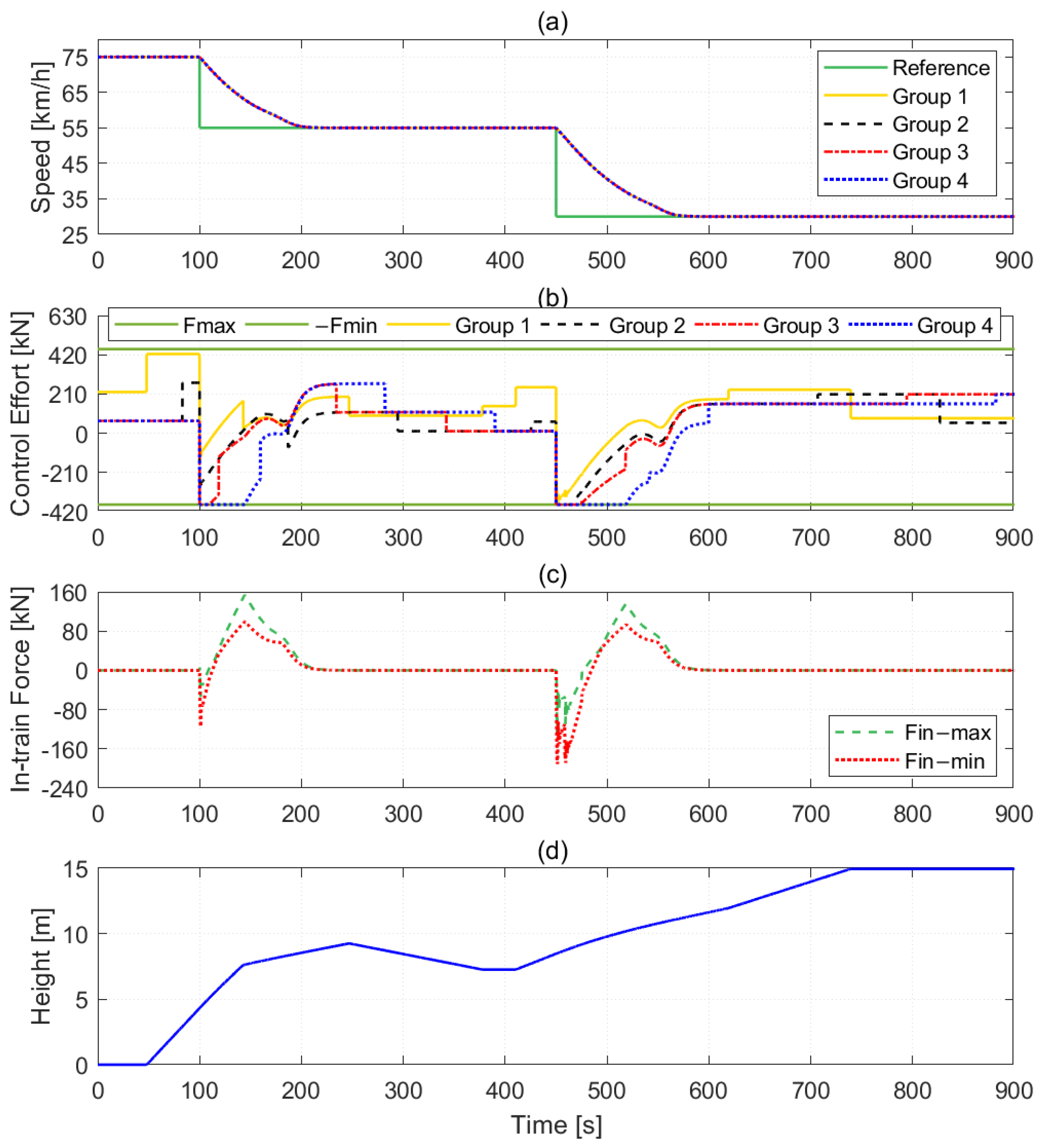
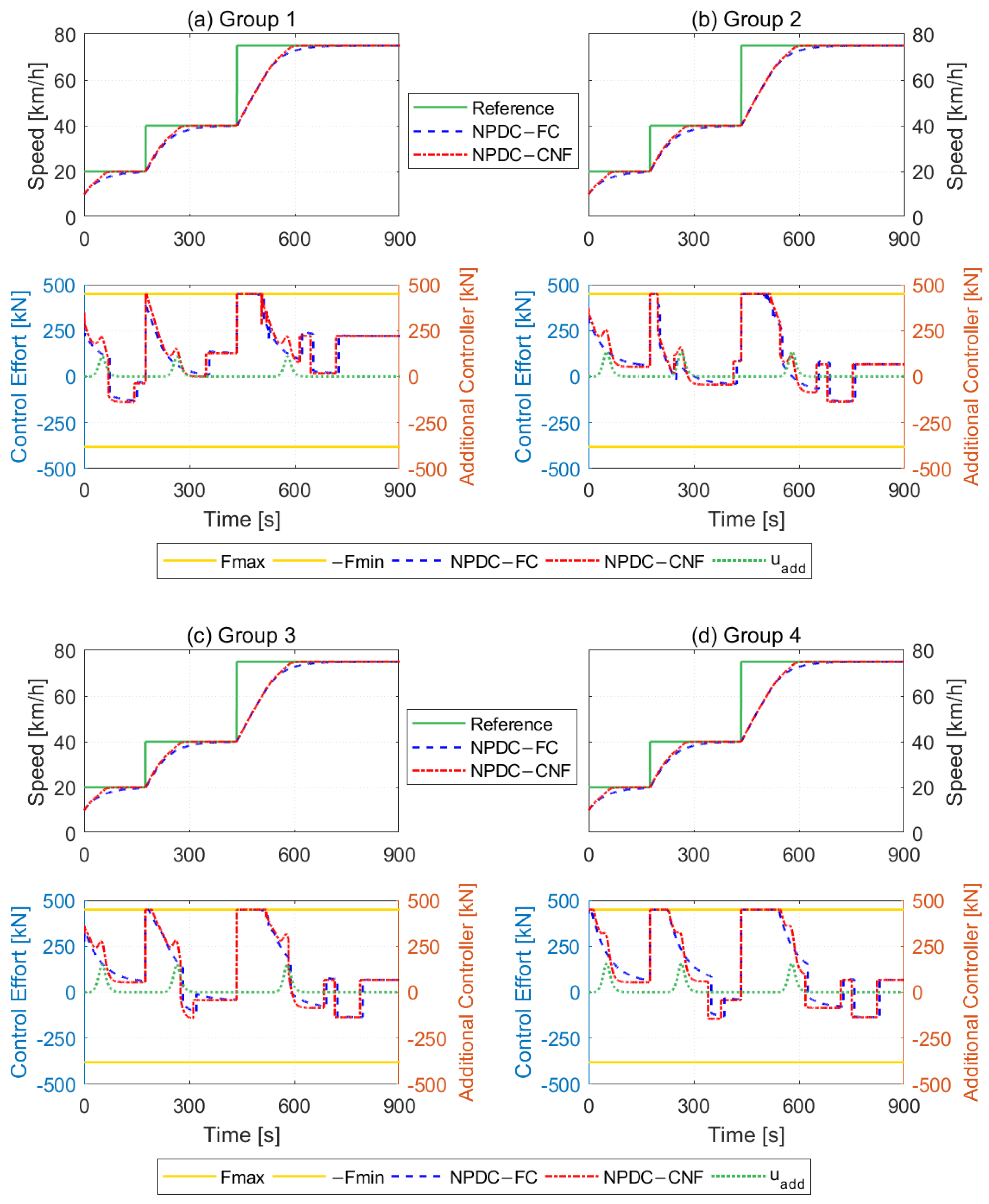
4.1. Performance of the Proposed Method

In this section, two simulation maneuvers are used to demonstrate the control performance of the presented strategy. The simulation results of maneuver 1 are shown in Figure 4, where the speed variation curves, control effort, the maximum and minimum in-train forces, and terrain topology are shown in sub-figures (a), (b), (c) and (d), respectively.

In this case, we assume that the initial speed of the heavy-haul train is 10 km/h, and the initial coupler displacements between adjacent groups are 0 m. In this paper, the tolerance band for speed tracking error is defined as 2% by referring to the classical control theory. Instead of using the traditional altitude—distance relationship curve to describe the rail track topology, this paper transforms it into an altitude—time curve to facilitate analysis of variations in traction/braking effort and speed as the slope changes over time. As shown in Figure 4a, each group starts to accelerate since the desired speed is 20 km/h during the period of [0, 175 s]. After about 72.8 s, all the speeds enter the steady state. When the desired speed rises to 40 km/h at 175 s, all speeds respond immediately, and about 104.6 s later, the higher reference speed is tracked. From 435 s, each group accelerates from 40 km/h to 75 km/h as the desired speed increases. All speeds converge to the equilibrium point at about 589.4 s.

According to (9) and the control input of the designed controller defined in Section 2.1, the control effort exerted on each group consists of the CNF control signal related to the state errors and the feedforward control signal counteracting the in-train force, the basic resistance, and the track slope resistance at the equilibrium point. Therefore, fluctuations in control efforts are inevitable due to the frequently changing track slope, as shown in Figure 4b. However, since downhill slopes are the majority in this maneuver, negative control inputs, i.e., braking efforts, are necessary to help each group maintain the desired speed. In addition, since the aerodynamic resistance is assumed to only act on the leading group, the control effort of group 1 is significantly different from others, which is shown clearly in steady states.

Meanwhile, the in-train forces vary with the changing reference speed, ranging from −287.4 kN to 88.55 kN. The maximum and minimum in-train forces share the same trend and converge to zero eventually, indicating that the proposed control strategy makes the spring-like couplers between adjacent groups remain at their natural length.

Furthermore, we validate the control performance of the controller under a deceleration maneuver. The simulation results are shown in Figure 5. Initially, the heavy-haul train travels at the reference speed of 75 km/h. After 100 s, the reference speed decreases to 55 km/h. Consequently, saturated braking forces are applied. The target speed is reached after about 92 s and maintained for 350 s. Then, the reference speed slows down further to 30 km/h. The train speed follows this trend and decreases to this speed within 109 s. As shown in Figure 5b, each control input experiences a change from negative to positive during each deceleration period. As the speed of each group approaches the reference speed gradually, the braking forces decrease to zero, and the control inputs become positive traction forces such that the speed of each group can remain at the current reference speed due to the uphill slopes. Throughout the running period, in-train forces are constrained in an appropriate range of [−191.1 kN,153.8 kN] from Figure 5c. In addition, each speed and in-train force converges to the equilibrium state almost at the same time.

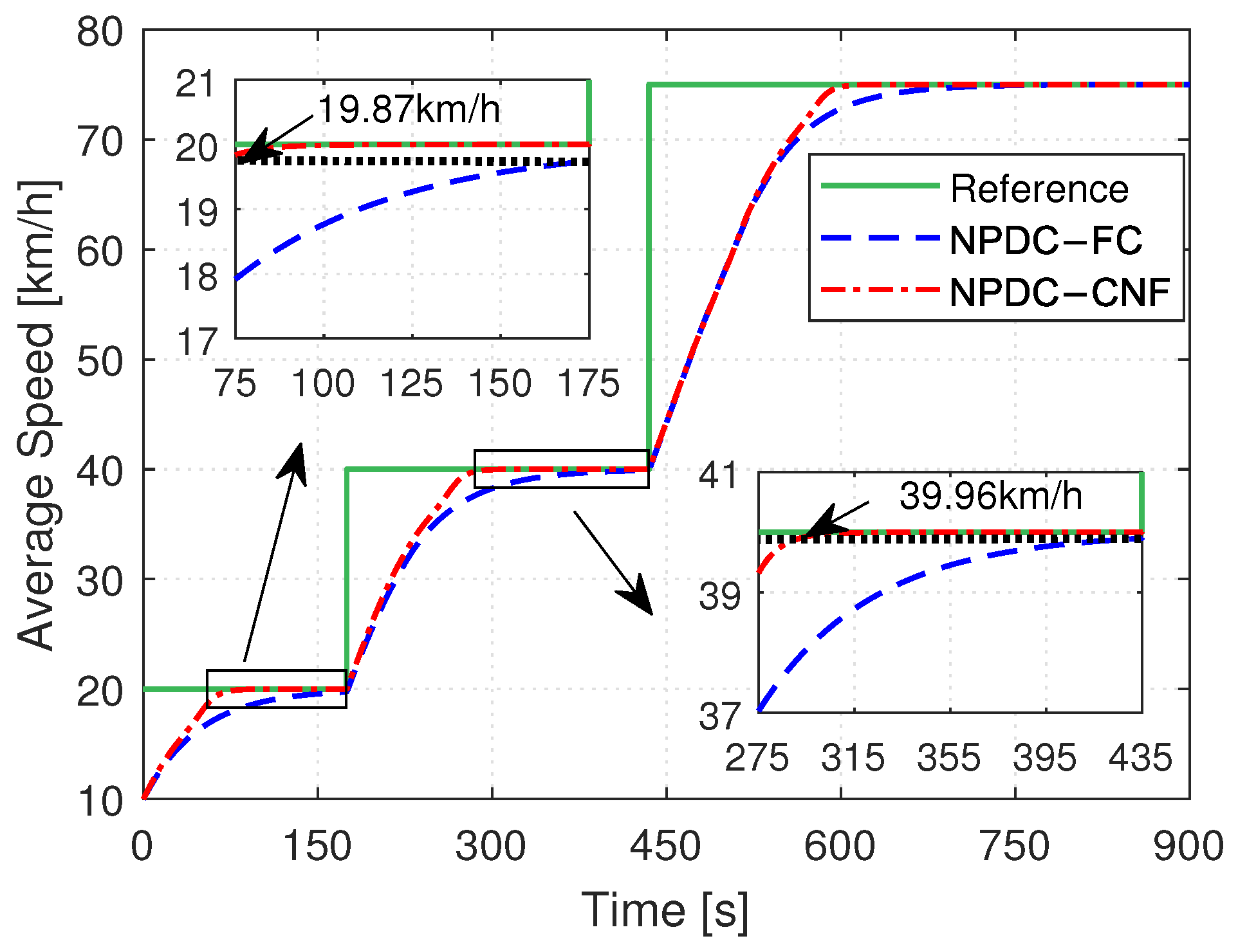
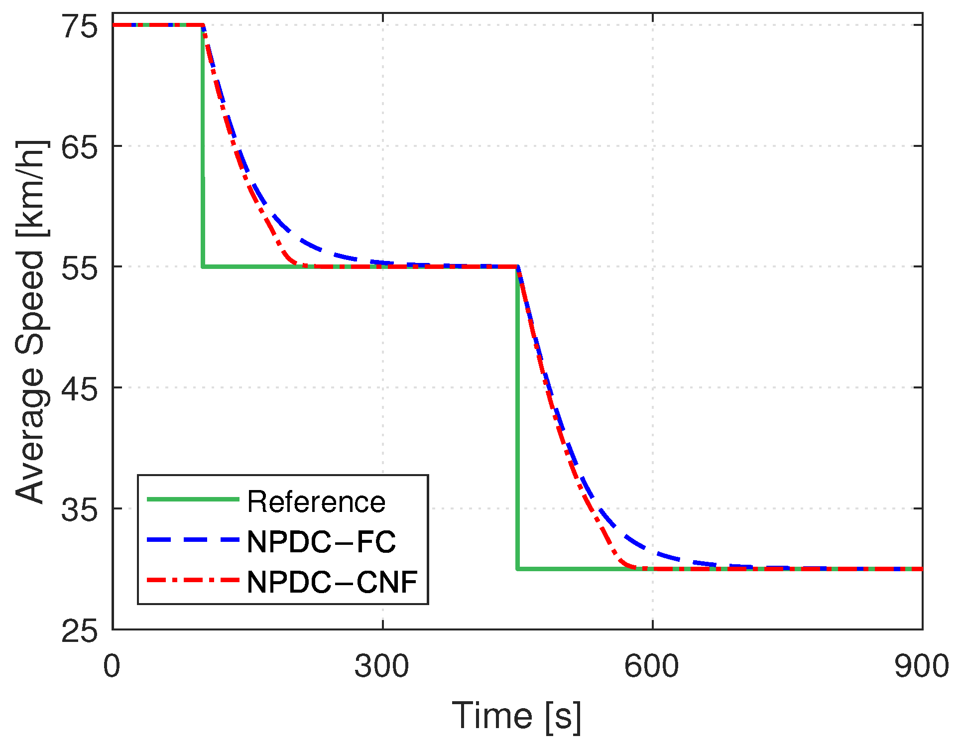
4.2. Comparison with Non-PDC Fuzzy Control Method

In order to demonstrate the superiority of the developed method, the non-PDC fuzzy controller is employed for comparison. For simplicity, we compare the average speed of the four groups for two different controllers. Figure 6 depicts the average speed of two methods, while Figure 7 shows four control inputs and speeds of two methods under Maneuver 1, as well as the additional control inputs of the proposed CNF controller. Figure 8 and Figure 9 demonstrate the deceleration comparison results. In these figures, the reference speed is denoted as “Reference”, the result of the proposed non-PDC fuzzy-based CNF controller and the non-PDC fuzzy controller are represented as “NPDC-CNF” and “NPDC-FC”, respectively, “${\mathrm{u}}_{\mathrm{add}}$” represents the output of the additional controller, and “Fmax” and “-Fmin” mark the upper and lower limits of the control input. In addition, the performance index comparison results of the speed tracking performance for acceleration and deceleration maneuvers are listed in

Table 2. Speed Tracking Performance Comparisons.

Maneuver	Running Time (s)	Settling Time (s) (2% Error Band)		Time to Equilibrium Point (s)
		NPDC CNF	NPDC FC	NPDC CNF	NPDC FC
Maneuver 1	0–175	72.8	156.3	105.6	>175
	175–435	104.6	166.9	143.4	>260
	435–900	154.4	198.7	198.1	391.7
Maneuver 2	0–100	0	0	0	0
	100–450	100.4	161.7	158.3	356.1
	450–900	117.5	172.6	158.3	356.1

.

As shown in Figure 6, both the proposed non-PDC fuzzy-based CNF controller and the non-PDC fuzzy control method can track the desired speed well under Maneuver 1. However, according to Table 2, the settling times of the proposed algorithm during each acceleration period are 72.8 s, 104.6 s, and 154.4 s, respectively, while for the non-PDC fuzzy control strategy, the corresponding times are 156.3 s, 166.9 s, and 198.7 s.

In addition, during the first acceleration period, the desired speed is tracked by the proposed method at 105.6 s, while there is a small steady-state tracking error of the non-PDC fuzzy method even at the end of the first acceleration period, i.e., the time to equilibrium point is more than 175 s. The same phenomenon happens in the second acceleration period. There is no doubt that the non-PDC fuzzy control has a larger steady-state speed tracking error compared with the proposed control method. Consequently, the proposed CNF controller improves transient performance and reduces the steady-state speed-tracking error for heavy-haul trains.

In Figure 7, the comparison results of four locomotive control efforts are depicted. One can observe that although the control inputs of the presented CNF method and the non-PDC fuzzy method have the same changing trends, there still exist some differences. By correlating the speed curves, control efforts curves and additional controller outputs curves, we can determine that, for each subgroup, the control effort of the CNF controller is not significantly different from that of the fuzzy controller during the initial acceleration period. However, as the speed approaches its set point, the additional controller of the CNF strategy $u_{add}$ becomes effective, leading to a noticeable improvement in speed regulation performance.

From Figure 8 and Figure 9 and Table 2, the proposed non-PDC fuzzy-based CNF method performs better than the non-PDC fuzzy strategy under Maneuver 2, which is similar to Maneuver 1.

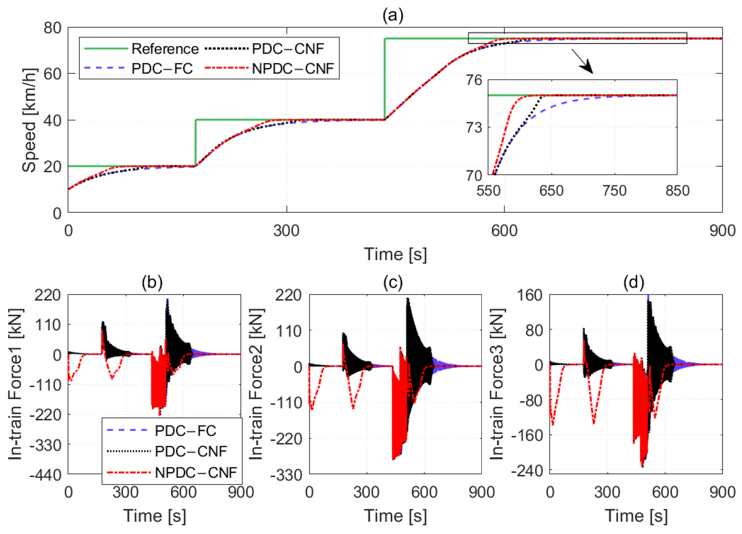
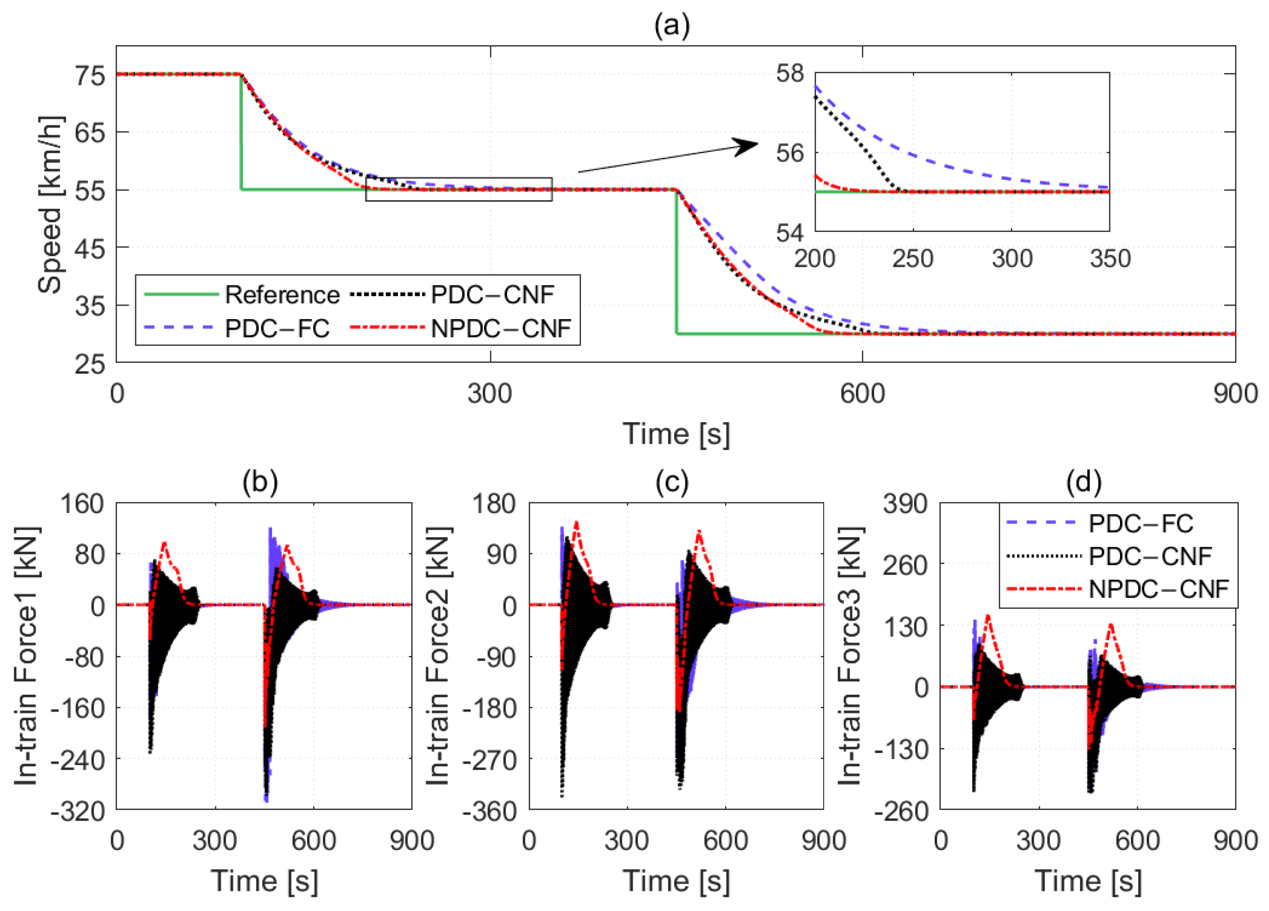
4.3. Comparison with PDC-Based Control Methods

In this section, we compare the control performance of the PDC fuzzy controller [21], the PDC-based CNF controller [26], and the proposed non-PDC fuzzy-based CNF controller. The simulation results for the average speed and in-train forces of three couplers under two maneuvers are presented in Figure 10 and Figure 11, where “PDC-FC” represents the PDC fuzzy controller, and “PDC-CNF” refers to the PDC-based CNF controller. The results indicate that the proposed non-PDC fuzzy-based CNF controller shows superior control performance, as it tracks the target speed more quickly and has smaller in-train forces. Ref. [33] attributed this phenomenon to the fact that more information about the simulation system is used by the non-PDC fuzzy-based controller than the PDC-based fuzzy controller. Additionally, the disturbance attenuation levels for the PDC-based CNF and non-PDC fuzzy-based CNF controllers are 0.0822 and 0.0127, respectively, which suggests that the closed-loop system demonstrates greater robustness due to the non-PDC fuzzy-based CNF controller. Moreover, the simulation comparison results between the PDC-based CNF controller and the PDC fuzzy controller reconfirm the effectiveness and superiority of the CNF algorithm in enhancing system transient performance.

In conclusion, simulation results qualitatively and quantitatively verify that the proposed CNF control strategy has apparent transient and steady-state performance enhancement capabilities.

5. Conclusions

A rapid response in speed tracking can significantly improve the transportation efficiency of heavy-haul trains. However, prior research on cruise control for these trains has primarily focused on steady-state performance, with inadequate attention to transient performance. To address this issue, we proposed a novel cruise control strategy aimed at improving transient performance while accounting for actuator saturation. A multi-particle error dynamics model was developed to capture the characteristics of heavy-haul trains. By applying the fencing concept and the T-S modeling method, we simplified the high-order nonlinear dynamics model into a low-dimensional fencing T-S model. Owing to the advantages of solving the input saturation and enhancing transient performance, we employed the CNF technique and designed a non-PDC fuzzy-based CNF controller. This novel controller offers a lower calculation burden and reduced conservativeness. Numerical simulation results validated the effectiveness of the proposed method and verified its capability for improving transient performance.

In future work, we may extend our strategy to heavy-haul trains equipped with ECP braking systems for long and steep downhill maneuvers while considering the limitations of in-train forces. Additionally, we will explore the analysis method of the feasible solution space for the proposed CNF controller.

References

1. Wang, X.; Su, S.; Cao, Y.; Qin, L.; Liu, W. Robust cruise control for the heavy haul train subject to disturbance and actuator saturation. IEEE Trans. Intell. Transp. Syst. 2023, 24, 8003–8013. [Google Scholar] [CrossRef]
2. Lu, Q.; He, B.; Wu, M.; Zhang, Z.; Luo, J.; Zhang, Y.; He, R.; Wang, K. Establishment and analysis of energy consumption model of heavy-haul train on large long slope. Energies 2018, 11, 965. [Google Scholar] [CrossRef]
3. Liu, W.; Tang, T.; Su, S.; Yin, J.; Cao, Y.; Wang, C. Energy-efficient train driving strategy with considering the steep downhill segment. Processes 2019, 7, 77. [Google Scholar] [CrossRef]
4. Zhang, W.; Sun, X.; Yang, S.; Yu, Z.; Wang, W.; Liu, Y. Optimization of speed curve for energy-saving of freight train based on equivalent gradient. In Proceedings of the 2021 IEEE International Intelligent Transportation Systems Conference (ITSC), Indianapolis, IN, USA, 19–22 September 2021; IEEE: Piscataway, NJ, USA, 2021; pp. 3438–3443. [Google Scholar] [CrossRef]
5. Zhuan, X.; Xia, X. Cruise control scheduling of heavy haul trains. IEEE Trans. Control Syst. Technol. 2006, 14, 757–766. [Google Scholar] [CrossRef]
6. Chou, M.; Xia, X. Optimal cruise control of heavy-haul trains equipped with electronically controlled pneumatic brake systems. Control Eng. Pract. 2007, 15, 511–519. [Google Scholar] [CrossRef]
7. Gao, K.; Huang, Z.; Wang, J.; Peng, J.; Liu, W. Decentralized control of heavy-haul trains with input constraints and communication delays. Control Eng. Pract. 2013, 21, 420–427. [Google Scholar] [CrossRef]
8. Zhang, L.; Zhuan, X. Optimal Operation of Heavy-Haul Trains Equipped with Electronically Controlled Pneumatic Brake Systems Using Model Predictive Control Methodology. IEEE Trans. Control Syst. Technol. 2014, 22, 13–22. [Google Scholar] [CrossRef]
9. Zhang, L.; Zhuan, X. Braking-penalized receding horizon control of heavy-haul trains. IEEE Trans. Intell. Transp. Syst. 2013, 14, 1620–1628. [Google Scholar] [CrossRef]
10. Zhang, L.; Zhuan, X. Development of an optimal operation approach in the MPC framework for heavy-haul trains. IEEE Trans. Intell. Transp. Syst. 2014, 16, 1391–1400. [Google Scholar] [CrossRef]
11. Wang, X.; Li, S.; Tang, T. Robust optimal predictive control of heavy haul train under imperfect communication. ISA Trans. 2019, 91, 52–65. [Google Scholar] [CrossRef]
12. Wang, X.; Li, S.; Tang, T. Periodically intermittent cruise control of heavy haul train with uncertain parameters. J. Frankl. Inst. 2019, 356, 6989–7008. [Google Scholar] [CrossRef]
13. Wang, X.; Li, S.; Tang, T. Robust efficient cruise control for heavy haul train via the state-dependent intermittent control. Nonlinear Anal. Hybrid Syst. 2020, 38, 100918. [Google Scholar] [CrossRef]
14. Zhuan, X.; Xia, X. Speed regulation with measured output feedback in the control of heavy haul trains. Automatica 2008, 44, 242–247. [Google Scholar] [CrossRef]
15. Zhu, B.; Xia, X. Nonlinear Trajectory Tracking Control for Heavy-Haul Trains. IFAC-PapersOnLine 2015, 48, 41–46. [Google Scholar] [CrossRef]
16. He, J.; Yang, X.; Zhang, C.; Liu, J.; Zhang, Q.; Chen, X. Tracking control via sliding mode for heavy-haul trains with input saturation. Meas. Control 2020, 53, 1720–1729. [Google Scholar] [CrossRef]
17. Wang, W.; Cui, K.; Lv, X.; Chang, M.; Gu, L. Automatic Train Operation for Heavy-Haul Trains Based on Adaptive Nonsingular Terminal Sliding Mode Control. In Proceedings of the 34th Chinese Control and Decision Conference (CCDC), Hefei, China, 15–17 August 2022; IEEE: Piscataway, NJ, USA, 2022; pp. 610–615. [Google Scholar] [CrossRef]
18. Huang, Y.; Bai, S.; Meng, X.; Yu, H.; Wang, M. Research on the driving strategy of heavy-haul train based on improved genetic algorithm. Adv. Mech. Eng. 2018, 10, 1687814018791016. [Google Scholar] [CrossRef]
19. Wang, X.; Li, S.; Tang, T.; Wang, X.; Xun, J. Intelligent operation of heavy haul train with data imbalance: A machine learning method. Knowl.-Based Syst. 2019, 163, 36–50. [Google Scholar] [CrossRef]
20. Liu, W.; Su, S.; Tang, T.; Wang, X. A DQN-based intelligent control method for heavy haul trains on long steep downhill section. Transp. Res. Part C Emerg. Technol. 2021, 129, 103249. [Google Scholar] [CrossRef]
21. Tanaka, K.; Wang, H.O. Fuzzy Control Systems Design and Analysis: A Linear Matrix Inequality Approach; John Wiley & Sons: Hoboken, NJ, USA, 2004. [Google Scholar] [CrossRef]
22. Wang, X.; Zhao, Y.; Tang, T. Fuzzy constrained predictive optimal control of high speed train with actuator dynamics. Discret. Dyn. Nat. Soc. 2016, 2016, 704743. [Google Scholar] [CrossRef]
23. Wang, X.; Tang, T. Optimal operation of high-speed train based on fuzzy model predictive control. Adv. Mech. Eng. 2017, 9, 1687814017693192. [Google Scholar] [CrossRef]
24. Chen, B.M.; Lee, T.H.; Peng, K.; Venkataramanan, V. Composite nonlinear feedback control for linear systems with input saturation: Theory and an application. IEEE Trans. Automat. Contr. 2003, 48, 427–439. [Google Scholar] [CrossRef]
25. Ebrahimi Mollabashi, H.; Mazinan, A.; Hamidi, H. Takagi–Sugeno fuzzy-based CNF control approach considering a class of constrained nonlinear systems. IETE J. Res. 2019, 65, 872–886. [Google Scholar] [CrossRef]
26. Hu, C.; Chen, Y.; Wang, J. Fuzzy observer-based transitional path-tracking control for autonomous vehicles. IEEE Trans. Intell. Transp. Syst. 2020, 22, 3078–3088. [Google Scholar] [CrossRef]
27. TB/T 1407.1-2018; Railway Train Traction Calculation Part 1: Trains with Locomotives. National Railway Administration of People’s Republic of China: Beijing, China, 2018. (In Chinese)
28. Vafamand, N.; Asemani, M.H.; Khayatiyan, A. A robust L1 controller design for continuous-time TS systems with persistent bounded disturbance and actuator saturation. Eng. Appl. Artif. Intell. 2016, 56, 212–221. [Google Scholar] [CrossRef]
29. Tuan, H.D.; Apkarian, P.; Narikiyo, T.; Yamamoto, Y. Parameterized linear matrix inequality techniques in fuzzy control system design. IEEE Trans. Fuzzy Syst. 2001, 9, 324–332. [Google Scholar] [CrossRef]
30. Duan, Z.; Ghous, I.; Shen, J. Fault detection observer design for discrete-time 2-D TS fuzzy systems with finite-frequency specifications. Fuzzy Sets Syst. 2020, 392, 24–45. [Google Scholar] [CrossRef]
31. Cao, Y.Y.; Lin, Z. Robust stability analysis and fuzzy-scheduling control for nonlinear systems subject to actuator saturation. IEEE Trans. Fuzzy Syst. 2003, 11, 57–67. [Google Scholar] [CrossRef]
32. Vazani, A.; Ghaffari, V. An innovative algorithm for tuning of composite nonlinear feedback control in continuous-time systems. Asian J. Control 2023, 25, 2295–2304. [Google Scholar] [CrossRef]
33. Zhao, L.; Li, L. Robust stabilization of T–S fuzzy discrete systems with actuator saturation via PDC and non-PDC law. Neurocomputing 2015, 168, 418–426. [Google Scholar] [CrossRef]
Figure 1. Longitudinal dynamics of heavy-haul train.
Electronics 14 02317 g001
Figure 2. Structure of the proposed CNF controller.
Electronics 14 02317 g002
Figure 3. Flowchart of the proposed cruise control algorithm.
Electronics 14 02317 g003
Figure 4. Cruise control results of Maneuver 1. (a) The speed tracking results of the four groups. (b) The control efforts of four groups. (c) The minimum and the maximum of the in-train forces. (d) The terrain topology.
Electronics 14 02317 g004
Figure 5. Cruise control results of Maneuver 2. (a) The speed tracking results of the four groups. (b) The control efforts of four groups. (c) The minimum and the maximum of the in-train forces. (d) The terrain topology.
Electronics 14 02317 g005
Figure 6. Average speed comparison result of Maneuver 1.
Electronics 14 02317 g006
Figure 7. Comparison results of the input and speed of each group under Maneuver 1. (a) The speed tracking results and control efforts of two control methods for group 1. (b) The speed tracking results and control efforts of two control methods for group 2. (c) The speed tracking results and control efforts of two control methods for group 3. (d) The speed tracking results and control efforts of two control methods for group 4.
Electronics 14 02317 g007
Figure 8. Average speed comparison result of Maneuver 2.
Electronics 14 02317 g008
Figure 9. Comparison results of the input and speed of each group under Maneuver 2. (a) The speed tracking results and control efforts of two control methods for group 1. (b) The speed tracking results and control efforts of two control methods for group 2. (c) The speed tracking results and control efforts of two control methods for group 3. (d) The speed tracking results and control efforts of two control methods for group 4.
Electronics 14 02317 g009
Figure 10. Comparison results of the PDC-based controllers and non-PDC fuzzy-based CNF controller under Maneuver 1. (a) The speed tracking results of three control methods. (b) The in-train forces of three control methods for coupler 1. (c) The in-train forces of three control methods for coupler 2. (d) The in-train forces of three control methods for coupler 3.
Electronics 14 02317 g010
Figure 11. Comparison results of the PDC-based controllers and non-PDC fuzzy-based CNF controller under Maneuver 2. (a) The speed tracking results of three control methods. (b) The in-train forces of three control methods for coupler 1. (c) The in-train forces of three control methods for coupler 2. (d) The in-train forces of three control methods for coupler 3.
Electronics 14 02317 g011