Abstract
Plant 3D reconstruction plays a critical role in precision agriculture and plant growth monitoring, yet it faces challenges such as complex background interference, difficulties in capturing intricate plant structures, and a slow reconstruction speed. In this study, we propose PlantSamGaussianReconstruction (PSGR), a novel method that integrates Grounding SAM with 3D Gaussian Splatting (3DGS) techniques. PSGR employs Grounding DINO and SAM for accurate plant–background segmentation, utilizes algorithms such as Scale-Invariant Feature Transform (SIFT) for camera pose estimation and sparse point cloud generation, and leverages 3DGS for plant reconstruction. Furthermore, a 3D–2D projection-guided optimization strategy is introduced to enhance segmentation precision. The experimental results of various multi-view plant image datasets demonstrate that PSGR effectively removes background noise under diverse environments, accurately captures plant details, and achieves peak signal-to-noise ratio (PSNR) values exceeding 30 in most scenarios, outperforming the original 3DGS approach. Moreover, PSGR reduces training time by up to 26.9%, significantly improving reconstruction efficiency. These results suggest that PSGR is an efficient, scalable, and high-precision solution for plant modeling.
1. Introduction
Plants are among the most diverse and widely distributed life forms on Earth, and their growth patterns, morphological characteristics, and ecological adaptations have long been subjects of scientific research [1]. In plant phenotyping studies, the observation of external plant morphology helps scientists quantitatively analyze growth patterns [2], disease responses, and adaptation mechanisms [3]. However, due to the complexity of plant growth environments, the irregularity of plant morphology, and the dynamic changes across different growth stages, traditional observation methods have significant limitations.
Observations and analyses of plants under various environmental and temporal conditions have revealed key features of their growth and adaptation mechanisms [4]. Long-term ecological studies have shown that plants exhibit remarkable plasticity in response to environmental factors [5]. For instance, rice demonstrates an adaptive root growth pattern under varying moisture conditions [6]. The response of plants to light is also highly noticeable; for example, certain fern species can adjust their leaf angles in low-light environments to maximize light absorption and maintain normal growth [7]. However, due to the vast diversity and complexity of plant species, the comprehensive recording and analysis of their growth states often face challenges, especially when dealing with complex or changing environments. To gain a deeper understanding of plant growth processes, an efficient, precise, and non-destructive reconstruction method is required that can observe various plants at different locations and times, supporting subsequent analysis.
Advances in digital [8] imaging technologies have provided new tools for plant phenotyping research. Two-dimensional (2D) image-based computational methods enable the non-contact and non-destructive measurement of basic plant morphological parameters, such as width, length, and area. However, these methods face limitations in capturing complex backgrounds or three-dimensional (3D) structures [9]. In contrast, 3D reconstruction technologies offer comprehensive geometric modeling tools [10], enabling the creation of high-precision 3D models of different plant species through standardized data collection. Current 3D reconstruction methods primarily rely on point clouds [11], voxels [12], and meshes [13]. Some research has made progress with a limited number of plant types. However, these methods usually rely on manual annotations or large-scale supervised data. Moreover, they face major challenges when dealing with complex backgrounds and irregular plant shapes. Furthermore, they are time-consuming, which severely restricts their application in scenarios requiring rapid results, such as real-time plant growth monitoring or large-scale plant phenotyping projects, where the long reconstruction time of traditional methods turns into a bottleneck.
During plant segmentation and 3D reconstruction, complex backgrounds may interfere with the extraction of features from the target plant, making it difficult to distinguish between the foreground and background. This can lead to mixed segmentation of the target plant and background, or result in partial loss of the target. Moreover, the growth patterns and structural characteristics of plants add to the modeling difficulty. Plant morphology is highly complex and variable, with leaves, stems, and other parts exhibiting diverse shapes and considerable structural differences. Traditional 3D reconstruction methods often struggle to capture these small features, potentially leading to incomplete or inaccurate models. Issues such as leaf gaps and occlusions further complicate the process. Gaps between leaves may result in data loss or reconstruction errors if not properly addressed. Additionally, overlapping and occluding leaves make it harder to obtain a complete 3D structure.
To address these challenges, especially the issue of slow reconstruction speed, this study proposes an innovative plant 3D reconstruction method. The method not only focuses on improving the reconstruction precision but also aims to significantly accelerate the 3D reconstruction process. It is designed to reduce the computational time required for plant 3D reconstruction without sacrificing accuracy, making it more suitable for practical applications. The objectives of this method are as follows: (1) A foreground segmentation method is proposed using Grounding SAM that accurately separates the plant from the background. This approach reduces background interference during 3D reconstruction, improving both segmentation quality and reconstruction efficiency. (2) A 3D–2D projection-guided optimization is introduced that utilizes 2D mask-based Gaussian ellipsoid projection. This enhances the background segmentation accuracy during 3D Gaussian Splatting, leading to more detailed and precise 3D reconstructions.
2. Related Work
Plant 3D reconstruction represents a crucial intersection between computer vision and agricultural information technology, aiming to generate high-precision 3D models of plants using multi-view imaging, depth sensing, or laser scanning technologies [14]. These reconstructions support precision agriculture, plant growth monitoring, and ecological studies. With the advancement of artificial intelligence (AI) and optical sensing technologies, the application scope of plant 3D reconstruction has significantly expanded to include crop phenotyping, pest and disease detection, and virtual ecosystem simulation [15]. Despite these developments, numerous challenges remain. The three-dimensional structures of plants often exhibit complex topologies, requiring reconstruction models to accurately capture fine-grained features such as leaves, stems, and their spatial hierarchies, while also distinguishing the geometric characteristics of different plant species. External factors such as complex backgrounds, occlusions (e.g., leaf overlapping), and data noise further complicate the reconstruction process. Therefore, improving the precision, robustness, and computational efficiency of plant 3D reconstruction remains a key challenge in the field.
Early plant reconstruction methods relied on rule-based models. For example, the L-system introduced by Lindenmayer [16] simulated plant growth topology but was limited in its ability to model real-world plant morphology. With the advent of non-contact sensing technologies, Light Detection and Ranging (LiDAR) became a tool for plant 3D modeling. Garcia et al. [17] utilized LiDAR scanning to obtain high-precision point clouds of crops, though the equipment was costly and sensitive to lighting conditions. Subsequently, computer vision-based methods emerged. Xu et al. [18] employed binocular stereo vision for reconstruction, but their approach struggled with variations in lighting and viewpoints, especially when reconstructing complex leaf structures. In recent years, multi-view reconstruction techniques such as Structure-from-Motion and Multi-View Stereo (SfM-MVS) [19] have become mainstream. Zhou et al. [20] used this approach to generate dense point clouds, significantly improving reconstruction accuracy. However, the method is computationally intensive and still suffers from occlusion problems. To address this, Liu et al. [21] incorporated PointNet and attention mechanisms to enhance the model’s ability to learn key structural features. Nevertheless, deep learning methods typically require large annotated datasets and considerable computational resources, which limits their practical applicability.
The field of 3D reconstruction has recently advanced through the use of differentiable rendering technologies. Neural Radiance Fields (NeRF) [22], employ multilayer perceptrons (MLPs) to map spatial coordinates and viewing angles to color and density, enabling a photorealistic view of synthesis via volumetric rendering. NeRF has demonstrated promise in plant phenotyping. However, its implicit representation limits its controllability and results in a slow training process, making high-resolution, real-time rendering difficult. In contrast, 3D Gaussian Splatting (3DGS) [23] uses explicit point cloud representations that support model storage and editing. By leveraging parallelized, differentiable rasterization pipelines, 3DGS achieves a high rendering efficiency while maintaining visual fidelity. While 3DGS is designed to deliver high-speed rendering and reconstruction, its application in plant modeling still faces challenges such as long optimization times and the need to manage occlusion. Furthermore, while 3DGS significantly outperforms NeRF in training and rendering speed, several hours of optimization are still required for high-precision reconstructions.
This study proposes a novel model called PSGR, which integrates Grounding Segment Anything Model (Grounding SAM) with 3DGS to achieve high-precision and accelerated plant modeling. The model structure is shown in Figure 1. The diagram illustrates the main stages of the framework, including segmentation, pose estimation, and 3D reconstruction. While not shown as a modular flowchart, the key components—such as 3D–2D projection-guided optimization—are integral to the reconstruction process and are further detailed in Section 3.1, Section 3.2, Section 3.3 and Section 3.4. The PSGR framework combines Grounding SAM, 3DGS, and 3D–2D-guided segmentation techniques to overcome background interference and improve the overall efficiency of 3DGS. First, Grounding SAM performs accurate plant object detection and initial segmentation, effectively separating the plant from a complex background. Then, the 3DGS method builds the 3D model, leveraging its unique point-based representation to capture the fine morphological details of the plant. Finally, a 3D–2D-guided segmentation strategy iteratively optimizes the geometric and texture fidelity between the reconstructed model and the original image data. By integrating PSGR’s efficient segmentation and background removal techniques, this multi-technique framework not only addresses traditional issues like background interference and low computational efficiency but also accelerates the overall reconstruction process. This results in faster training and rendering, making it well-suited for real-time or large-scale plant modeling tasks, while significantly enhancing both the accuracy and generalizability of plant 3D reconstruction.
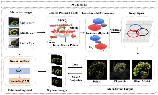
Figure 1.
Conceptual overview of the PSGR pipeline.
3. Methods
3.1. Accurate Plant Background Segmentation Based on Grounding DINO and the Segment Anything Model
Traditional 3D reconstruction generally aims to restore entire scenes using multi-view images as input. However, this study focuses on reconstructing a 3D model of a single plant specimen. To achieve this, we propose an innovative integration of Grounding DINO [24] and the Segment Anything Model (SAM) [25] for precise background removal in multi-view plant images. This hybrid approach allows for the effective isolation of the target plant even in complex environments, thereby providing clean, background-free images that serve as a reliable foundation for subsequent 3D visualization and rendering.
Grounding DINO is an open-vocabulary object detection model based on a Transformer architecture [26]. Unlike conventional detectors that rely on predefined categories, Grounding DINO formulates object detection as a sequence prediction task and uses textual prompts for visual grounding. In our application, prompts such as “a single plant” or “a maize plant” can be input to the model to automatically locate and draw bounding boxes around the target plant. The detection process of Grounding DINO is illustrated in Figure 2.
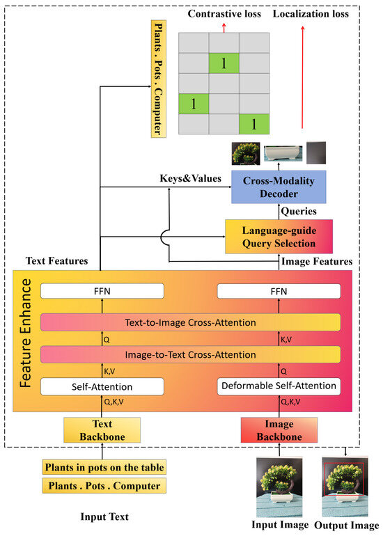
Figure 2.
The object detection process of Grounding DINO. The text and the image are respectively encoded into feature vectors through the Text Backbone and the Image Backbone. They are fused by multiple layers of modules, including self-attention. The language-guided mechanism extracts target words from the text and guides the cross-modal decoder to locate regions in the image. Detection is completed based on the matching degree between the detected objects and the text prompts.
To robustly detect plants under various conditions, such as inconsistent lighting, occlusions, or cluttered backgrounds, Grounding DINO employs a Transformer-based matching loss computed using the Hungarian algorithm to find the optimal assignment between predicted and ground truth objects. The optimization objective is formulated in Equation (1) using Hungarian matching. The individual loss components are defined in Equation (2), and the total loss is described in Equation (3):
where denotes the set of all possible match permutations, and is the matching cost that measures the discrepancy between predicted and ground truth objects. Specifically, represents the classification loss, is the L1 loss for bounding box regression, and denotes the generalized Intersection-over-Union (GIoU) loss. The coefficients , , and are weighting factors that balance the contributions of different loss terms.
This mechanism enables Grounding DINO to generate highly accurate bounding boxes under varied and challenging field or laboratory conditions, thereby supporting reliable plant background segmentation for SAM-based instance mask generation.
This study takes a set of multi-view plant images captured from different angles as input and performs object detection using Grounding DINO. Based on predefined textual prompts, Grounding DINO automatically identifies and generates bounding boxes for the target plant, accurately localizing its position and outputting the detection results. These bounding boxes, along with their corresponding image crops, are then passed to the SAM for further processing.
The SAM segmentation model [25] can automatically perform instance segmentation guided by various types of prompts. Compared with conventional segmentation approaches, SAM demonstrates a strong generalization ability and can adapt to various plant types, lighting conditions, and background complexities without requiring additional training. Specifically, SAM utilizes a powerful image encoder [27] to extract features from the input image. It applies a Transformer-based architecture to convert the entire image into a high-dimensional feature representation, in which spatial information and visual content are encoded into vectors suitable for model interpretation.
By incorporating a self-attention mechanism, SAM effectively captures the long-range spatial dependencies within the image, which is critical for fine-grained segmentation tasks. The self-attention operation is typically defined as in Equation (4):
where Q, K, and V denote the query, key, and value matrices, respectively, and represents the dimensionality of the key vectors. This mechanism enables the model to capture correlations between distant pixels, which is particularly beneficial for object segmentation.
In the context of multi-view plant 3D reconstruction, where background complexity poses significant challenges, we leverage the open-vocabulary Transformer-based object detector Grounding DINO to compute object matching and total training loss, thereby achieving precise plant localization and bounding box generation. These outputs are subsequently fed into the SAM model, which uses its powerful visual encoder and self-attention mechanism to perform fully automated plant region segmentation. As a result, only the target plant is retained while background noise is removed. This ensures clean, interference-free, multi-view inputs, significantly improving the precision and efficiency of the subsequent 3D visualization and rendering.
3.2. Camera Pose Estimation and Sparse Point Cloud Generation
Camera pose estimation and sparse point cloud generation are core procedures in the 3D reconstruction pipeline. The former estimates the camera’s position and orientation in 3D space to ensure multi-view image alignment, while the latter reconstructs 3D scene points via triangulation, serving as the foundation for dense reconstruction. These processes critically affect the overall accuracy and quality of the reconstruction results. Accordingly, this module is divided into four sequential steps: feature extraction, feature matching, camera pose estimation, and sparse point cloud generation.
Initially, the Scale-Invariant Feature Transform (SIFT) [28] is employed to detect keypoints at multiple scales using the Difference of Gaussian (DoG) pyramid. Each keypoint is encoded into a 128-dimensional orientation histogram descriptor. The local orientation normalization mechanism embedded in SIFT ensures robustness against variations in scale, in-plane rotation, and illumination, thus providing reliable 2D–2D correspondences across views and enhancing the baseline stability of the reconstruction system.
Subsequently, Approximate Nearest Neighbor (ANN) search and Lowe’s ratio test are applied for feature matching. Geometric consistency is then validated using RANSAC [29] to effectively reject outliers. This ensures reliable feature correspondences between image pairs, supporting accurate camera pose estimation and scene recovery.
Based on the matching results, the Perspective-n-Point (PnP) algorithm [30] is applied in conjunction with RANSAC to estimate the extrinsic parameters of newly introduced camera views using existing 3D–2D correspondences. The PnP problem is formulated as the minimization of the reprojection error, as expressed in Equation (5):
where denotes a 3D point in world coordinates, is its corresponding 2D image projection, R and t represent the camera’s rotation and translation, and is the projection function. This objective function minimizes the sum of the squared distances between the observed 2D points and the projected 3D points, yielding optimal camera pose estimation. To further enhance geometric consistency, global camera trajectories and scene structure are refined using Structure-from-Motion (SfM) and Bundle Adjustment (BA). These procedures improve pose accuracy and provide a stable foundation for triangulation.
Finally, triangulation is performed to recover 3D point positions, followed by BA optimization of both the sparse point cloud and the camera parameters. The resulting sparse reconstruction serves as the initialization for Multi-View Stereo (MVS), playing a crucial role in improving the accuracy and completeness of the final 3D model.
3.3. Gaussian Splatting-Based Plant Reconstruction
To achieve high-precision and high-fidelity 3D plant modeling, this study adopts a multi-view reconstruction approach based on 3D Gaussian splatting. The method consists of three key stages: the initialization of 3D Gaussian ellipsoids, rasterization-based Gaussian rendering, and the density regulation of Gaussian points. The initial plant point cloud is used to initialize Gaussians, generating Gaussian ellipsoids for leaves and flowers. These are projected using camera poses and processed through adaptive density control. A tile-based rasterizer then renders the final plant image. The overall workflow is illustrated in Figure 3.
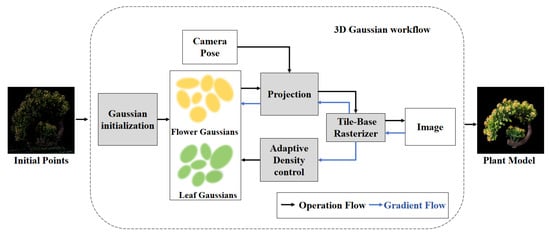
Figure 3.
Workflow of 3D Gaussian splatting.
3.3.1. Initialization of 3D Gaussian Points
Each sparse point obtained from the previous reconstruction step is initialized as a 3D Gaussian ellipsoid. Specifically, for every point in the sparse cloud, a 3D Gaussian function is constructed to model both its spatial location and shape. These 3D Gaussian distributions are mathematically defined in Equation (6):
where x is a 3D spatial coordinate, denotes the mean vector encoding the position of the Gaussian center, and is the covariance matrix representing the shape and orientation of the ellipsoid. To simplify matrix operations and preserve the positive semi-definite property, the covariance matrix is factorized into a rotation matrix R and a scaling matrix S, as shown in Equation (7):
Geometrically, this factorization represents first aligning the ellipsoid with the world coordinate system via rotation, and then scaling it along the principal axes and rotating it back.
3.3.2. Splatting and Rendering in Plant Reconstruction
After obtaining the 3D Gaussian ellipsoids, the next step is to project them onto the 2D image plane for rendering. The fundamental idea is to project each 3D Gaussian point using the camera parameters, generating a set of 2D Gaussian distributions that are blended to synthesize the final image. We adopt the Elliptical Weighted Average (EWA) filtering technique, which uses a local affine transformation to approximate the projection of 3D Gaussians, as shown in Equation (8):
where W is the view transformation matrix (mapping from world to camera coordinates), J is the Jacobian of the affine approximation, and is the resulting 2D covariance matrix on the image plane.
During rendering, each pixel is covered by N 2D Gaussian distributions. According to the physical imaging principle, closer objects occlude those farther away. In volume rendering, this principle is modeled by sorting the Gaussians in depth order and performing front-to-back alpha compositing. The final color c of a pixel is computed by aggregating the contributions of sorted Gaussians, as shown in Equations (9) and (10):
where denotes the color of the i-th Gaussian, and is the updated opacity. The term encodes the occlusion effect by accumulating the transparency from preceding Gaussians in depth order. Larger values result in reduced contribution from subsequent Gaussians.
Based on the computed color and opacity, Gaussian splats are rendered from different viewpoints to generate the final image. This enables flexible 3D visualization from arbitrary camera angles and facilitates the construction of complete 3D digital plant models.
3.3.3. Density Control of 3D Gaussian Points
In the initial stage, 3D Gaussian splatting relies solely on the sparse point cloud for constructing Gaussian ellipsoids. However, the rendering quality of the final 3D plant model is directly affected by the density of Gaussian points. Merely optimizing the parameters of existing Gaussian points is insufficient to achieve the desired rendering performance. When the current Gaussians fail to adequately cover the reconstruction domain, cloning operations are applied to duplicate existing ellipsoids. Conversely, when the coverage is coarse, splitting operations are used to refine the point distribution. Each 3D Gaussian ellipsoid is associated with an opacity parameter. To reduce unnecessary computational load and maintain rendering quality, ellipsoids with opacities below a predefined threshold are discarded. This process effectively increases the number of meaningful Gaussian points in 3D space while removing those with negligible rendering contribution, thereby significantly improving both rendering quality and computational efficiency.
3.4. 3D–2D Projection-Guided Background Segmentation Optimization
In the process of 3D plant reconstruction, overlapping between foreground plants and the background in 2D images can result in coarse segmentation if grounding DINO and SAM are applied without refinement. Moreover, issues such as leaf occlusions and internal holes further degrade reconstruction quality. To address this challenge, we propose a 3D–2D Projection-Guided (3D–2D PG) background optimization strategy in Figure 4. The Gaussian distribution is projected onto the image plane, with each Gaussian ellipsoid having a different projection range, indicated in blue. The red regions represent areas that are irrelevant to the target segmentation. After optimization, the Gaussians belonging to the target are marked in blue, while those not belonging to the target are marked in red. This approach incorporates a projection-guided Gaussian ellipse masking mechanism into the 3DGS pipeline to improve segmentation fidelity and enhance the quality of 3D plant models.
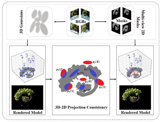
Figure 4.
3D–2D projection-guided method. The effectiveness of this method is demonstrated through visualization.
Given a specific 3D Gaussian point cloud , its projection onto image plane I forms a 2D ellipse. A high-quality 2D mask provided by Grounding SAM is used as supervisory information. We analyze the spatial relationship between the projected ellipse and the 2D mask in three cases: (1) intersection—partial overlap between projection and target region; (2) containment—projection fully lies within the target region; and (3) exclusion—projection lies entirely within the background.
To quantify this relationship, we define the 3D–2D Projection Consistency Score (3D–2D PS) in Equation (11):
where i denotes the index of the 3D Gaussian, j refers to the index of a specific query, represents the 2D mask region, and denotes the 2D projection of the 3D Gaussian. A higher value indicates better alignment between the projected Gaussian and the ground truth target region, and thereby serves as a guide to improve projection-aware segmentation refinement.
During training, the PSGR model renders 2D images from the current 3D Gaussian ellipsoid configuration via differentiable splatting. The rendered images are then compared with the corresponding ground-truth views to compute reconstruction losses. These losses are backpropagated through the splatting operation to update Gaussian parameters (position, orientation, color, and opacity). Additionally, the 3D–2D projection-guided consistency score serves as an auxiliary supervision term that refines the selection and optimization of Gaussians, especially in background filtering. By jointly leveraging image-level losses and projection-based geometric alignment, the model is able to suppress irrelevant structures and enhance the fidelity of the reconstructed plant models.
4. Experiments
4.1. Plant and Image Acquisition
To validate the effectiveness of the proposed method, multi-view image datasets of various plant species were collected in two distinct environments: indoor potted settings and outdoor potted settings. Three commonly cultivated ornamental plants were selected for analysis, namely Ctenanthe setosa (Grey Star Ctenanthe), Sansevieria trifasciata ‘White Jade’ (Snake Plant), and Pachira aquatica (Money Tree). Image acquisition was conducted in two stages from three different viewpoints. In the first stage, each plant was photographed from a top view, a front view, and an upward view to capture its overall structure. In the second stage, close-up images focusing on key structural components and fine-grained phenotypic features were obtained.To increase the diversity of image acquisition sources and improve the generalizability of the proposed method, multiple smartphone models from different manufacturers were employed. These included the iPhone 13 Pro, Redmi K50, Redmi K80, and Huawei Nova 7 SE.
4.2. Experimental Environment and Evaluation Metrics
All model training and evaluation procedures were conducted on the same workstation, configured with the following hardware specifications: a 64-bit Windows operating system, a 12th Gen Intel(R) Core(TM) i5-12490F CPU (Intel, Santa Clara, CA, USA) operating at 3.00 GHz, and an NVIDIA GeForce RTX 4060 GPU (NVIDIA, Santa Clara, CA, USA) with 16 GB of memory. The software environment included Anaconda v3.4, Python v3.7.13, CUDA v11.8, and PyTorch v1.21.1.
To ensure reproducibility and clarify the training configurations, we provide the key hyperparameter settings used in all experiments. The optimization was performed for 30,000 iterations using the Adam optimizer. The learning rates were set to 0.001 for position, 0.01 for color, and 0.1 for opacity. The opacity threshold for pruning Gaussian ellipsoids was fixed at 0.005. Gaussian splitting was conducted every 2000 iterations to enhance coverage. Additionally, in the 3D–2D projection-guided optimization module, the consistency score threshold was set to 0.6 to filter background projections. All experiments were performed using the same random seed to maintain reproducibility.
To rigorously assess the effectiveness of our plant 3D reconstruction framework, we adopted a set of standard yet diverse metrics targeting both visual quality and computational performance. We evaluated reconstruction fidelity by computing the peak signal-to-noise ratio (PSNR), mean absolute error (MAE), and L1 loss between the synthesized views and their corresponding ground-truth images. The final scores were averaged over all test perspectives to obtain a holistic measurement. The PSNR metric reflects the logarithmic proportion between the highest possible pixel intensity and the mean squared deviation, with higher scores indicating superior perceptual similarity. MAE, on the other hand, measures the average of absolute per-pixel differences, offering robustness to local anomalies. The L1 loss further complements this by summing the pixel-wise absolute deviations, thus reflecting the fine-grained rendering precision. Moreover, the total training duration was recorded to represent the method’s computational footprint. Given the computational demands of 3D reconstruction tasks, training time serves as a critical indicator of method practicality. As such, we particularly value the efficiency with which our approach completes the reconstruction process. To ensure fairness in comparative evaluations, all experiments were conducted in identical hardware environments. Collectively, these indicators enable a comprehensive and balanced assessment of both the visual realism and processing efficiency involved in recovering plant geometries from multi-view input.
4.3. Ablation Study
To evaluate the contributions of the individual components in the proposed PSGR plant 3D reconstruction model, we conducted a series of ablation experiments by removing key modules. The results of these experiments are summarized in Table 1.

Table 1.
Results of the ablation experiment with 30,000 iterations at a 50 k point cloud scale.
The ablation experiment was conducted under a 50 k point cloud scale, using the original 3DGS [23] as the baseline model, with a PSNR of 29.72 and a time cost of 4130 s. After incorporating the Grounding SAM foreground segmentation module, the time cost decreased by 27.55%, and the PSNR improved to 31.87, indicating a significant acceleration effect while maintaining and even enhancing reconstruction quality. When the 3D–2D-guided optimization module was added, the time cost slightly increased, but the impact on overall reconstruction time was negligible. This module effectively improved the reconstruction accuracy, increasing the PSNR to 33.25.
The ablation results confirm that the Grounding SAM foreground segmentation module is crucial for speeding up the 3D reconstruction process while maintaining high reconstruction quality. Removing this module significantly increases the processing time. The 3D–2D-guided optimization also contributes to accuracy but has a lesser impact on time efficiency compared to Grounding SAM. Overall, the full PSGR model provides the best trade-off between speed and quality.
4.4. Visualization Experimental Results of Plants
4.4.1. Foreground Segmentation of Plants
By integrating Grounding DINO [24] with the SAM segmentation model [25], our approach enables accurate background removal for most plants across diverse environments, resulting in cleanly segmented plant foregrounds. Figure 5 illustrates the processing pipeline using the Grounding SAM framework on a plant captured in an arbitrary setting. Given an input image containing a plant and a textual prompt “plant”, Grounding DINO first detects and highlights the region corresponding to the plant. Subsequently, Grounding SAM refines the detection and performs precise segmentation. The final output image clearly presents the isolated foreground plant, demonstrating the effectiveness of the proposed method in complex visual scenes.
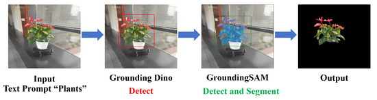
Figure 5.
Visualization workflow of Grounding SAM.
4.4.2. Comparison Between 3D Gaussians and PSGR
Figure 6 and Figure 7 presents a comprehensive visual comparison between 3DGS and PSGR across three plant species—Grey Star Ctenanthe, Snake Plant, and Money Tree—under both indoor and outdoor conditions. From a qualitative perspective, the PSGR model demonstrates markedly improved visual clarity. It achieves more effective background removal, significantly reduces visual artifacts, and enhances the preservation of fine structural details. These improvements enable the clear observation of morphological features such as leaf curvature and spatial topology, which are often obscured or lost in conventional 3DGS outputs.
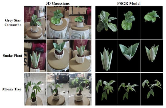
Figure 6.
Visual comparison of original 3D Gaussians and PSGR for three indoor plants.
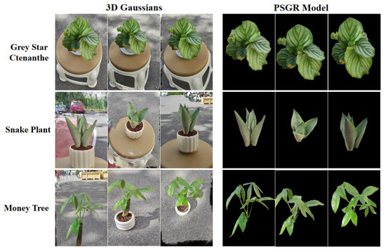
Figure 7.
Visual comparison of original 3D Gaussians and PSGR for three outdoor plants.
To quantitatively compare PSGR with 3DGS across different environmental conditions, we computed the loss, mean absolute error (MAE), and peak signal-to-noise ratio (PSNR) for all three plant species in both indoor and outdoor settings, at 7000 and 30,000 training iterations. As shown in Table 2 and Table 3, PSGR consistently maintains high PSNR values across all stages and plant types. Notably, in indoor environments—where lighting is more controlled and background interference is lower—PSGR achieves PSNR values exceeding 38 for Snake Plant and Money Tree, and maintains a strong performance even for Grey Star Ctenanthe. In more challenging outdoor scenarios, where background complexity and lighting variability are higher, PSGR still achieves a PSNR above 30 in most cases. This confirms its robustness in handling real-world noise and structural occlusions. Although PSGR shows a slightly lower PSNR in a few cases compared to 3DGS, particularly for Grey Star Ctenanthe, it overall demonstrates more stable and high-fidelity reconstruction results across varied environmental conditions. These results quantitatively support PSGR’s adaptability to both indoor and outdoor plant modeling tasks.
Table 2.
The results for three kinds of indoor potted plants at the 7000th iteration and the 30,000th iteration.
Table 3.
The results for three kinds of outdoor potted plants at the 7000th iteration and the 30,000th iteration.
Table 4 and Figure 8 illustrate the reconstruction training times of PSGR and 3DGS under various initial point cloud scales. The last row shows the percentage of time reduction achieved by PSGR compared to 3DGS at 30,000 iterations. The results show that PSGR significantly accelerates the training process across all tested configurations. Specifically, as the number of initial point clouds increases from 5 k to 50 k, PSGR consistently achieves notable reductions in training time, with improvements ranging from 15.4% to 26.9% at the 30,000 iteration mark. This substantial time efficiency highlights the scalability and computational advantage of our method, making it highly suitable for time-sensitive or large-scale plant reconstruction applications.
Table 4.
Comparison of time consumption (in seconds) between 3DGS and PSGR under different numbers of initial point clouds at 7000 and 30,000 training iterations.
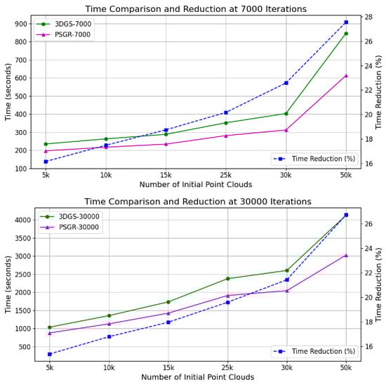
Figure 8.
Time consumption and reduction comparison between 3DGS and PSGR.
To assess computational efficiency, we compare PSGR and 3DGS under varying point cloud sizes. As shown in Table 5, PSGR achieves 25–33% faster inference across all scales. It also reduces both model size and output volume significantly. For example, at 50 k, the model file shrinks from 396 MB to 211 MB, and the output from 136 MB to 72.9 MB. These results demonstrate PSGR’s superior speed and memory efficiency while maintaining high reconstruction quality.
Table 5.
Comparison of model size, parameter count, inference time, and output file size under varying point cloud scales.
The experimental results demonstrate that the PSGR model achieves a robust reconstruction performance in both indoor and outdoor environments, effectively reducing background interference and preserving fine plant details. PSGR offers improved visual fidelity compared to baseline 3DGS while significantly accelerating the training process. These advantages make it a practical and scalable solution for plant structural modeling in diverse and complex conditions.
4.4.3. Comparative Visualization of Plants in Various Scenes
To further evaluate the performance of PSGR, we conducted a comparative experiment with Instant-NGP [31] and the original NeRF model. The comparison includes both qualitative and quantitative results based on three plant species captured in indoor and outdoor environments. As shown in Figure 9, PSGR produces clearer and more detailed reconstructions than the NeRF-based methods. Table 6 further quantifies these differences, showing that PSGR achieves the highest PSNR across all settings while maintaining a significantly reduced training time compared to original NeRF.
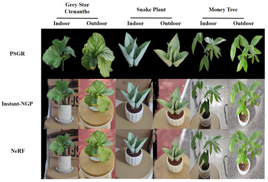
Figure 9.
Visual comparison of the PSGR, Instant-NGP, and NeRF of three plant species under indoor and outdoor scenes.
Table 6.
Comparison of PSNR (dB) and time consumption (min) across three reconstruction methods under different plants and environments.
In terms of image quality, PSGR produces sharper and more structurally accurate reconstructions. Its precise background removal preserves clear plant contours and fine leaf details. In contrast, NeRF often suffers from leaf blurring and detail loss under occlusion or low-texture conditions. While Instant-NGP is faster, it sacrifices visual quality—edges appear blurred and the plant often merges with the background. PSGR overcomes these issues, delivering cleaner, well-separated, and more interpretable 3D reconstructions across diverse environments.
In terms of computational efficiency, Instant-NGP achieves significantly shorter training times compared to PSGR. This is primarily attributed to its internal use of hash-encoded neural representations, which fundamentally differ from PSGR’s explicit point-based modeling and optimization strategy. While this design allows Instant-NGP to accelerate reconstruction, it inherently compromises structural fidelity to some extent. Notably, PSGR maintains high reconstruction accuracy while still substantially outperforming NeRF in terms of efficiency. For instance, in the indoor reconstruction of Grey Star Ctenanthe, NeRF requires up to 374 min, whereas PSGR completes the process in only 8.03 min, demonstrating remarkable computational efficiency.
In summary, compared with conventional NeRF-based plant 3D reconstruction methods, PSGR demonstrates clear advantages. By effectively eliminating background interference through precise foreground segmentation and 3D-2D projection-guided optimization, our method ensures cleaner inputs for reconstruction. Meanwhile, PSGR consistently achieves higher PSNR values across various plant types and environments, indicating improved image fidelity. Most notably, it significantly reduces training time while maintaining high reconstruction accuracy, offering a practical and scalable solution for large-scale plant phenotyping applications.
5. Discussion
The 3DGS technique represents a significant breakthrough in the field of 3D reconstruction. It has achieved remarkable results in various domains, particularly in large-scale scene reconstruction and object modeling, where its point-cloud-based representation improves rendering efficiency while maintaining high visual fidelity. However, the potential of 3DGS in the agricultural plant domain remains underexplored. The structural complexity of plants and the variability of their growing environments present unique challenges for 3D reconstruction.
While our proposed framework leverages Grounding SAM for foreground segmentation, it is important to note that our primary research objective is to improve the precision and efficiency of 3D plant reconstruction. The segmentation component is a supporting mechanism to enhance reconstruction quality by reducing background interference. As such, we adopted the Grounding DINO + SAM combination for its open-vocabulary and fine-grained segmentation capabilities, without conducting extensive comparisons with other segmentation approaches such as YOLO-based models. In future work, we plan to evaluate how different foreground extraction methods may affect overall reconstruction performance in order to further assess the robustness and generalizability of our approach.
This study utilized small potted plants for the experimental tests, with the initial point cloud data ranging from 5 k to 50 k points. In practical applications, variations in plant morphology and size may result in larger point clouds, especially when processing high-resolution images or more complex environments, where the point cloud size may reach up to millions of points. As image quality improves, the number of point clouds will increase, which, while potentially raising computational time, will also make the acceleration effects of the proposed method more pronounced. Therefore, future research can further validate the effectiveness of this method in plant 3D reconstruction.
6. Conclusions
This study proposed a novel plant 3D reconstruction framework PSGR, which combines Grounding SAM, 3D Gaussians, and a 3D–2D projection-guided segmentation refinement strategy. The PSGR pipeline effectively addresses key challenges in plant reconstruction, including complex background interference and the need for fine-grained structural preservation. The experimental results demonstrate that PSGR achieves consistently high reconstruction fidelity across multiple plant species and environmental settings. Specifically, PSGR maintains PSNR values above 30 in most scenarios and outperforms the original 3DGS method in terms of both PSNR and MAE metrics. In addition to its visual quality improvements, PSGR also delivers a significant reduction in computational time—achieving up to 26.9% faster training under large-scale point cloud configurations—thereby enhancing its applicability in time-sensitive or large-scale phenotyping tasks. Overall, these results highlight PSGR as a robust, efficient, and scalable solution for high-precision plant modeling. Future research will explore extensions toward temporal consistency across growth stages, the integration of multimodal sensing modalities, and deployment in large-scale in-field phenotyping systems to support intelligent agricultural decision-making and data-driven breeding programs.
Author Contributions
Conceptualization: J.C. and Y.J.; Methodology: J.C. and Y.J.; Software: J.C. and Y.J.; Validation: J.C., Y.J. and F.J.; Formal Analysis: J.C., Y.N. and Y.J.; Investigation: J.C. and Y.J.; Resources: J.C. and Y.J.; Data Curation: J.C. and Y.J.; Writing—Original Draft Preparation: J.C. and Y.J.; Writing—Review and Editing: J.C., Y.J. and Y.Z.; Visualization: J.C. and Y.J.; Supervision: Y.J. and M.Y.; Project Administration: Y.J. and M.Y.; Funding Acquisition: X.Q. All authors have read and agreed to the published version of the manuscript.
Funding
This work was supported by the Guangxi Key Research and Development Program (AB25069476, AB24010164, AB23026048), the Beijing Natural Science Foundation (F2024205028), the Hebei Natural Science Foundation (F2024205028), and the Guilin Science and Technology Project (20230112-1, 20230104-6).
Institutional Review Board Statement
Not applicable.
Informed Consent Statement
Not applicable.
Data Availability Statement
Data are contained within the article.
Conflicts of Interest
The authors declare no conflicts of interest.
References
- Antonelli, A.; Govaerts, R.; Nic Lughadha, E.; Onstein, R.E.; Smith, R.J.; Zizka, A. Why plant diversity and distribution matter. New Phytol. 2023, 240, 1331–1336. [Google Scholar] [CrossRef] [PubMed]
- Noshita, K.; Murata, H.; Kirie, S. Model-based plant phenomics on morphological traits using morphometric descriptors. Breed. Sci. 2022, 72, 19–30. [Google Scholar] [CrossRef] [PubMed]
- Schneider, H.M. Characterization, costs, cues and future perspectives of phenotypic plasticity. Ann. Bot. 2022, 130, 131–148. [Google Scholar] [CrossRef] [PubMed]
- Adams, W.W., III; Stewart, J.J.; Polutchko, S.K.; Cohu, C.M.; Muller, O.; Demmig-Adams, B. Foliar phenotypic plasticity reflects adaptation to environmental variability. Plants 2023, 12, 2041. [Google Scholar] [CrossRef]
- Brooker, R.; Brown, L.K.; George, T.S.; Pakeman, R.J.; Palmer, S.; Ramsay, L.; Schöb, C.; Schurch, N.; Wilkinson, M.J. Active and adaptive plasticity in a changing climate. Trends Plant Sci. 2022, 27, 717–728. [Google Scholar] [CrossRef]
- Yamauchi, T.; Pedersen, O.; Nakazono, M.; Tsutsumi, N. Key root traits of Poaceae for adaptation to soil water gradients. New Phytol. 2021, 229, 3133–3140. [Google Scholar] [CrossRef]
- Khan, I.; Sohail; Zaman, S.; Li, G.; Fu, M. Adaptive responses of plants to light stress: Mechanisms of photoprotection and acclimation. A review. Front. Plant Sci. 2025, 16, 1550125. [Google Scholar] [CrossRef]
- Omari, M.K.; Lee, J.; Faqeerzada, M.A.; Joshi, R.; Park, E.; Cho, B.K. Digital image-based plant phenotyping: A review. Korean J. Agric. Sci. 2020, 47, 119–130. [Google Scholar] [CrossRef]
- Luo, L.; Jiang, X.; Yang, Y.; Samy, E.R.A.; Lefsrud, M.; Hoyos-Villegas, V.; Sun, S. Eff-3DPSeg: 3D organ-level plant shoot segmentation using annotation-efficient point clouds. arXiv 2022, arXiv:2212.10263. [Google Scholar]
- Okura, F. 3D modeling and reconstruction of plants and trees: A cross-cutting review across computer graphics, vision, and plant phenotyping. Breed. Sci. 2022, 72, 31–47. [Google Scholar] [CrossRef]
- Sun, G.; Wang, X. Three-dimensional point cloud reconstruction and morphology measurement method for greenhouse plants based on the kinect sensor self-calibration. Agronomy 2019, 9, 596. [Google Scholar] [CrossRef]
- Feng, J.; Saadati, M.; Jubery, T.; Jignasu, A.; Balu, A.; Li, Y.; Attigala, L.; Schnable, P.S.; Sarkar, S.; Ganapathysubramanian, B.; et al. 3D reconstruction of plants using probabilistic voxel carving. Comput. Electron. Agric. 2023, 213, 108248. [Google Scholar] [CrossRef]
- Paproki, A.; Sirault, X.; Berry, S.; Furbank, R.; Fripp, J. A novel mesh processing based technique for 3D plant analysis. BMC Plant Biol. 2012, 12, 63. [Google Scholar] [CrossRef]
- Yang, D.; Yang, H.; Liu, D.; Wang, X. Research on automatic 3D reconstruction of plant phenotype based on Multi-View images. Comput. Electron. Agric. 2024, 220, 108866. [Google Scholar] [CrossRef]
- Zhou, L.; Wu, G.; Zuo, Y.; Chen, X.; Hu, H. A comprehensive review of vision-based 3d reconstruction methods. Sensors 2024, 24, 2314. [Google Scholar] [CrossRef]
- Lindenrnayer, A. Mathematical models for cellular interactions in development. J. Theor. Biol. 1968, 18, 280–315. [Google Scholar] [CrossRef]
- Garcia, M.; de Souza, M.; Gebbers, R.; Peets, S.; Cielniak, G.; Hämmerle, M.; Bennertz, D.; Tang, L.; Andújar, D.; Tsiropoulos, Z. LiDAR-based point cloud acquisition for crop modeling: Precision and challenges. Comput. Electron. Agric. 2020, 175, 105579. [Google Scholar]
- Xu, J.; Ma, Y.; Liang, Y.; Guan, Y.; Luo, X.; Cui, S.; Zhang, H.; Fan, J.; Wang, S. Binocular stereo vision for plant 3D reconstruction: Challenges and solutions. Comput. Electron. Agric. 2019, 158, 184–192. [Google Scholar]
- Schonberger, J.L.; Frahm, J.M. Structure-from-motion revisited. In Proceedings of the IEEE Conference on Computer Vision and Pattern Recognition, Las Vegas, NV, USA, 27–30 June 2016; pp. 4104–4113. [Google Scholar]
- Zhou, Z.; Li, Y.; Xue, Z.; Luo, Z.; Zhang, X.; Xu, J.; Chen, Q.; Li, R.; Tang, Y.; Wang, Z. Multi-view reconstruction techniques in plant modeling: A review and comparison. Comput. Biol. Med. 2022, 137, 104794. [Google Scholar]
- Liu, Z.; Zhao, C.; Wang, L.; Liu, Y.; Xu, Y.; Zhao, Y.; Wang, H.; Li, C.; Wang, J.; Zhang, L. PointNet-based 3D plant reconstruction with attention mechanisms. Comput. Electron. Agric. 2021, 182, 105968. [Google Scholar]
- Mildenhall, B.; Srinivasan, P.P.; Tancik, M.; Barron, J.T.; Ramamoorthi, R.; Ng, R. Nerf: Representing scenes as neural radiance fields for view synthesis. Commun. ACM 2021, 65, 99–106. [Google Scholar] [CrossRef]
- Kerbl, B.; Kopanas, G.; Leimkühler, T.; Drettakis, G. 3D Gaussian splatting for real-time radiance field rendering. ACM Trans. Graph. 2023, 42, 1–14. [Google Scholar] [CrossRef]
- Liu, S.; Zeng, Z.; Ren, T.; Li, F.; Zhang, H.; Yang, J.; Jiang, Q.; Li, C.; Yang, J.; Su, H.; et al. Grounding dino: Marrying dino with grounded pre-training for open-set object detection. In European Conference on Computer Vision; Springer: Cham, Switzerland, 2024; pp. 38–55. [Google Scholar]
- Kirillov, A.; Mintun, E.; Ravi, N.; Mao, H.; Rolland, C.; Gustafson, L.; Xiao, T.; Whitehead, S.; Berg, A.C.; Lo, W.Y.; et al. Segment anything. In Proceedings of the IEEE/CVF International Conference on Computer Vision, Paris, France, 1–6 October 2023; pp. 4015–4026. [Google Scholar]
- Vaswani, A.; Shazeer, N.; Parmar, N.; Uszkoreit, J.; Jones, L.; Gomez, A.N.; Kaiser, Ł.; Polosukhin, I. Attention is all you need. Adv. Neural Inf. Process. Syst. 2017, 30, 5998–6008. [Google Scholar]
- Dosovitskiy, A.; Beyer, L.; Kolesnikov, A.; Weissenborn, D.; Zhai, X.; Unterthiner, T.; Dehghani, M.; Minderer, M.; Heigold, G.; Gelly, S.; et al. An image is worth 16 × 16 words: Transformers for image recognition at scale. arXiv 2020, arXiv:2010.11929. [Google Scholar]
- Lowe, D.G. Object recognition from local scale-invariant features. In Proceedings of the seventh IEEE International Conference on Computer Vision, Kerkyra, Greece, 20–27 September 1999; Volume 2, pp. 1150–1157. [Google Scholar]
- Fischler, M.A.; Bolles, R.C. Random sample consensus: A paradigm for model fitting with applications to image analysis and automated cartography. Commun. ACM 1981, 24, 381–395. [Google Scholar] [CrossRef]
- Lepetit, V.; Moreno-Noguer, F.; Fua, P. EPnP: An accurate O(n) solution to the PnP problem. Int. J. Comput. Vis. 2009, 81, 155–166. [Google Scholar] [CrossRef]
- Müller, T.; Evans, A.; Schied, J.; Keller, A. Instant Neural Graphics Primitives with a Multiresolution Hash Encoding. ACM Trans. Graph. 2022, 41, 102:1–102:15. [Google Scholar] [CrossRef]
Disclaimer/Publisher’s Note: The statements, opinions and data contained in all publications are solely those of the individual author(s) and contributor(s) and not of MDPI and/or the editor(s). MDPI and/or the editor(s) disclaim responsibility for any injury to people or property resulting from any ideas, methods, instructions or products referred to in the content. |
© 2025 by the authors. Licensee MDPI, Basel, Switzerland. This article is an open access article distributed under the terms and conditions of the Creative Commons Attribution (CC BY) license (https://creativecommons.org/licenses/by/4.0/).