Building Electricity Prediction Using BILSTM-RF-XGBOOST Hybrid Model with Improved Hyperparameters Based on Bayesian Algorithm

Abstract

Accurate building energy consumption prediction is essential for efficient energy management and energy optimization. This study utilizes bidirectional long short-term memory (BiLSTM) to automatically extract deep time series features. The nonlinear fitting and high-precision prediction capabilities of Random Forest (RF) and XGBoost models are then utilized to develop a BiLSTM-RF-XGBoost stacked hybrid model. To enhance model generalization and reduce overfitting, a Bayesian algorithm with an early stopping mechanism is utilized to fine-tune hyperparameters, and strict K-fold time series cross-validation (TSCV) is implemented for performance evaluation. The hybrid model achieves a high TSCV average R² value of 0.989 during cross-validation. When evaluated on an independent test set, it yields a mean square error (MSE) of 0.00003, a root mean square error (RMSE) of 0.00548, a mean absolute error (MAE) of 0.00130, and a mean absolute percentage error (MAPE) of 0.26%. These values are significantly lower than those of comparison models, indicating a significant improvement in predictive performance. The study offers insights into the internal decision-making of the model through SHAP (SHapley Additive exPlanations) feature significance analysis, revealing the key roles of temperature and power lag features, and validating that the stacked model effectively utilizes the outputs of base models as meta-features. This study makes contributions by proposing a novel hybrid model trained with Bayesian optimization, analyzing the influence of various feature factors, and providing innovative technological solutions for building energy consumption prediction. It also provides theoretical value and guidance for low-carbon building energy management and application.

1. Introduction

Sustainable social development has led to an increasing number of buildings in all walks of life, while economic growth and human development have also brought about rapid growth in energy consumption [1]. Electricity, as an energy resource that is generated, transmitted, planned, and distributed to users, is a necessary resource and strong support for the development of market economies and industrial research and progress [2]. How to reasonably plan the use of electricity resources is critical to energy conservation, emission reduction, and low-carbon green development, and it is also a necessary means to promote social development. Electricity consumption forecasting is an important measure in resource planning, which can effectively help improve energy utilization, reduce energy consumption costs, and improve equipment management [3]. Accurate electricity consumption forecasting can avoid redundant energy waste [4]. With the development of industry, energy consumption forecasting has gradually become more important than ever [5]. Energy consumption forecasting can generally be divided into short-, medium-, and long-term forecasting according to the time range [6]. For building power consumption prediction, short-term prediction with a time range of 3–7 days can not only accurately provide the trend of power consumption, but also assist managers in making timely responses to regulate power consumption so as to achieve the goal of building energy-saving and emission reduction [7].

Most buildings that rely heavily on electricity for energy consumption not only consume a huge amount of electricity but also are affected by factors such as temperature, time, holidays, etc. Power consumption data generally has the characteristics of high dimensionality, high volatility, and nonlinear non-stationarity. For energy consumption prediction, researchers usually use traditional linear statistical methods, grey system models, intelligent deep learning, and machine learning models [8]. Traditional linear models, such as ARIMA, AR, MA, and other models, are based on the assumption that all time series are stationary and linear. These traditional research methods cannot cope with the prediction challenges posed by highly complex electricity consumption data [9], which can lead to prediction bias and reduced prediction accuracy. Although traditional models such as RNN and SVR can model the correlation between nonlinear data to improve prediction accuracy, the drawback of these models is that the input and output are independent when processing data, ignoring the potential dependence between energy consumption data, which leads to a decrease in prediction accuracy and difficulty in developing the potential of the model [10]. Studies have demonstrated that bidirectional long short-term memory networks (BILSTMs) are a suitable method for achieving predictions [11]. They can not only effectively handle long-term dependencies in time series data but also identify complex, nonlinear relationships between learning input features, which are difficult for traditional models to deal with.

However, the existing research tends to focus on the optimization of a single model, ignoring the potential of model combination and the significant impact of hyperparameters on model performance. It is difficult for a single model to adequately capture the complex patterns in the data when facing the challenges of high data dimensionality and complex, nonlinear relationships in building electricity forecasting [12]. In the field of complex time series prediction and pattern recognition, model fusion and hierarchical processing strategies show notable advantages. For example, in the study of unmanned aerial vehicle (UAV) trajectory prediction [13], Shi emphasized the importance of flight state-based recognition. They significantly improved the accuracy of trajectory prediction by first accurately identifying the flight states (e.g., climbing, leveling, and hovering) of UAVs, and then constructing independent prediction models for different states.

In addition, most researchers in the field have favored the use of fixed hyperparameters, which may lead to inefficient results because the a priori process of hyperparameters is usually quite complex when facing a high-dimensional parameter space [14], and it is difficult to obtain the optimal model performance with fixed hyperparameters. Therefore, an approach that can combine the advantages of multiple models and select optimal hyperparameters to improve the accuracy and robustness of predictive forecasting is of research interest, and hybrid models often outperform single models [15].

In terms of fine-grained modeling for specific application domains, ZhuoYong Shi et al.’s study on the design of a motor skill recognition and hierarchical assessment system for table tennis players successfully demonstrated the importance of combining fine-feature engineering and pattern recognition [16]. They realized the accurate determination of athletes’ skill level by constructing a database of action features and combining it with a machine learning model for skill recognition and multilevel assessment. The idea of multi-dimensional feature construction and hierarchical assessment in this study has some commonality with the proposed hierarchical feature learning and decision-making mechanism through multi-scale temporal feature derivation as well as stacking model in this study, both aiming to capture the behavioral patterns of complex systems from different granularities and levels. And data fusion technology plays a key role in some recognition tasks that rely on multi-source information. In ZhuoYong Shi et al.’s study on the design of UAV flight state recognition system based on multi-sensor data fusion, the accuracy and robustness of UAV flight state recognition are improved by effectively integrating data from different sensors [17]. Together, these related studies confirm the effectiveness of using decomposition, layering, and fusion strategies to deal with multi-dimensional and multi-scale information in complex system modeling, and also provide theoretical references and methodologies for the construction of hybrid models proposed in the follow-up of this study.

In summary, aiming to make up for the shortcomings of the existing building electricity prediction methods, this study novelly develops a hybrid model of BILSTM-RF-XGBOOST based on Bayesian improved hyperparameters in order to make full use of the advantages of each model, and more crucially, the study implements a strict K-fold time series cross-validation (Time Series Cross- Validation (TSCV). This approach ensures that hyperparameters are chosen based on the average performance of the model over multiple consecutive time periods rather than a single validation split, thus significantly reducing the risk of overfitting and improving the generalization ability of the model. Finally, the model is evaluated on a completely independent test set to verify its true performance. Bayesian optimization methods have been used to efficiently improve model hyperparameters for optimal predictive performance [14].

Contribution

The main contributions of this study are shown as follows:

• A new hybrid model is proposed by integrating the advantages of three single models, which can effectively deal with the complex characteristics of high-dimensional, high-noise and nonlinear energy consumption data.
• The model hyperparameters are improved by a Bayesian algorithm to overcome the limitations of traditional methods while achieving optimal model performance.
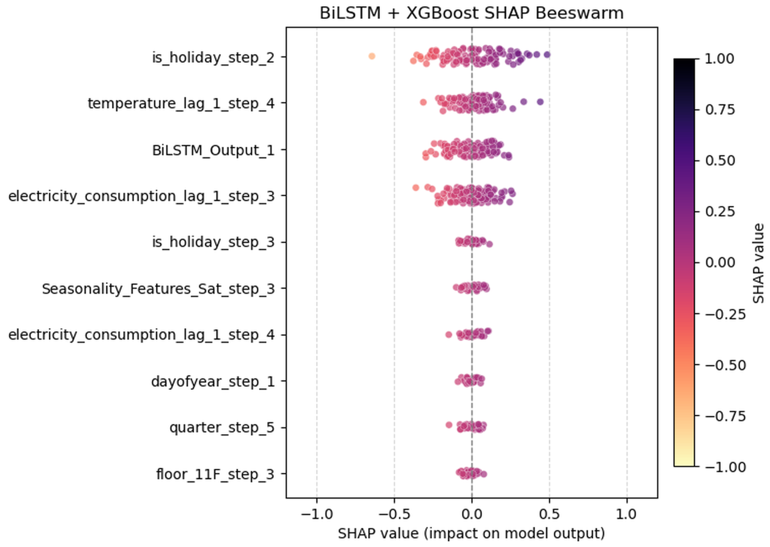
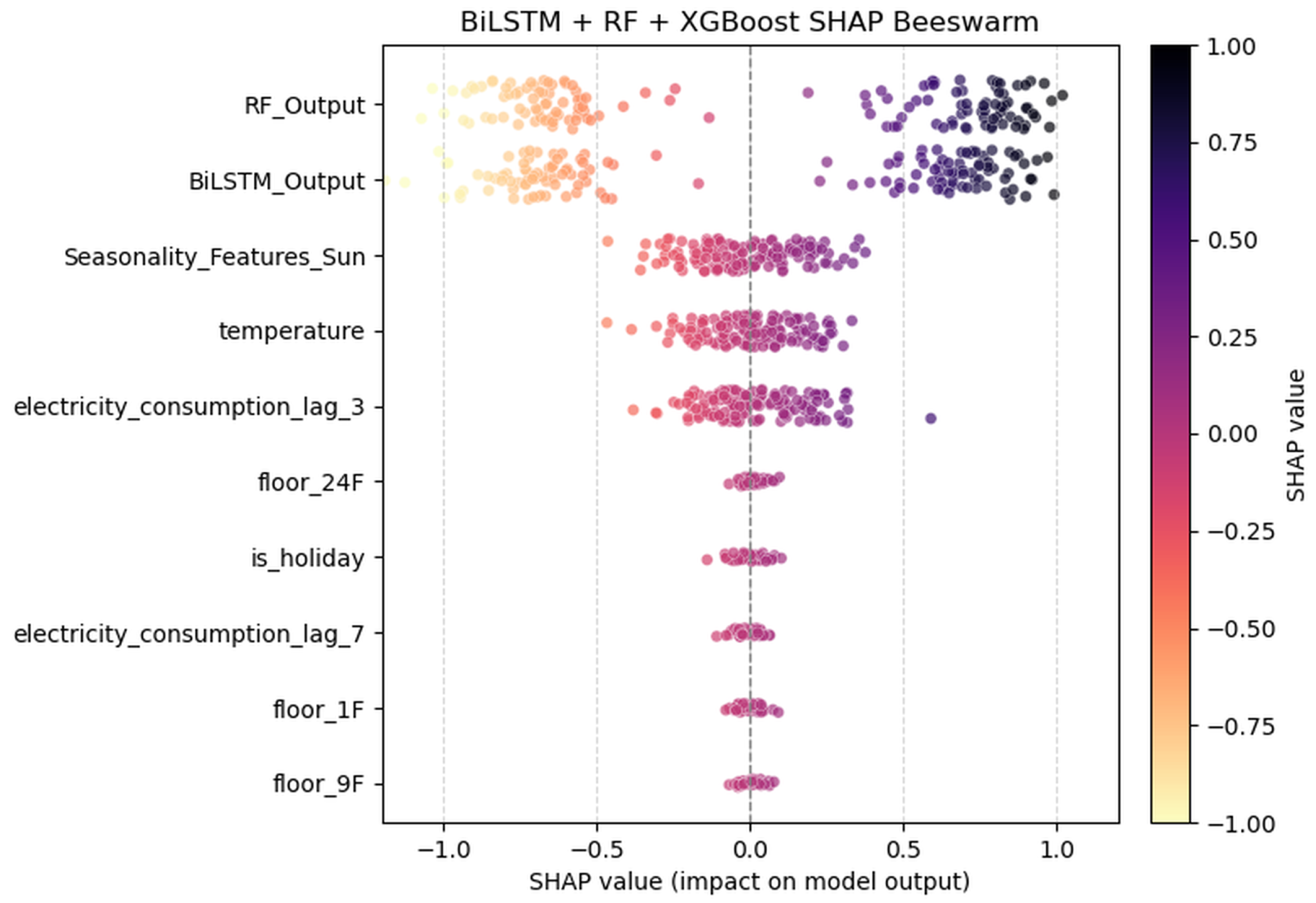
• Using SHAP as the main tool for feature significance analysis reveals the key factors affecting electricity consumption, quantifies the positive and negative influence of different feature factors on model predictions, and provides a transparent and reliable basis for the development of energy management strategies.

2. Related Work

Electricity consumption forecasting is crucial for the stable development of the power industry and the rational operation of the energy system. In previous studies by scholars such as Mehmet Bilgili and Engin Pinar, a single long short-term memory network LSTM was used to predict total electricity consumption, and the LSTM prediction was verified to be more accurate through comparison with the SARIMA model. However, the comparison of too few model types is not convincing. The research only used a single form of power data and failed to fully incorporate important external factors affecting power consumption, so it cannot prove the universality of the LSTM model [2]. Andrea Maria N. C. Ribeiro and Pedro Rafael X. do Carmo used various single models such as ARIMA to predict energy consumption. After determining the optimal configuration of model parameters through grid search, they found that the GRU model performed well. However, the disadvantage is that although grid search hyperparameters are used, the efficiency and effectiveness are limited by the preset search space, especially in the high-dimensional hyperparameter space, where grid search may miss a better model configuration [3]. Namrye Son and Yoonjeong Shin et al. proposed a short- to medium-term electricity consumption prediction algorithm by combining the GRU model with the prophet model, which can help save a significant amount of electricity costs and reduce carbon emissions. The disadvantage is that this fusion strategy is mainly based on empirical observation and intuition, and lacks a more in-depth theoretical analysis to support the rationality and effectiveness of this fusion [8]. Fang Liu and Chen Liang et al. proposed the AC-BILSTM model for electricity compliance prediction, which was optimized using the random search method (RSM). The prediction performance and accuracy were demonstrated under different time steps. However, the features used in the paper are relatively basic, and the deep factors of effective electricity compliance were not fully explored. In addition, the RSM method is still based on a preset range, which has the hidden problem of the global optimal solution not being explored [10]. Shu Cheng Luo and Qing Zhong Gao and others used a stacked ensemble algorithm based on CNN-BILSTM and XGBOOST to predict short-term power loads, and successfully applied this algorithm to the Quanzhou area. However, the drawback is that the model performance is affected by obvious temperature changes, and it is still unable to cope with the hyperparameter adjustment mechanism. The accuracy and validity of the prediction results under some extreme conditions are affected by this [12]. Chao Tang, Yufeng Zhang and others developed a data-driven power load model using a hybrid model of CNN-BILSTM for experimental comparison under uncertain power conditions, which confirmed the effectiveness of the CNN-BILSTM model in predicting power loads under uncertain conditions. However, the research process only briefly mentioned the hyperparameter setting, and lacked a detailed description of the hyperparameter optimization process, which makes the reproducibility of the experimental results and the scientific nature of the model optimization process slightly insufficient [6]. Zi Qing Yu and Shuai Yuan et al. stacked and integrated the XGBOOST-BILSTM model for power load prediction, making full use of the mastery of BILSTM of the long-term dependence of past and future data, and using XGBOOST to compensate for interpretability, successfully improving the accuracy of load prediction. However, the study did not thoroughly explore the interpretability of the model in the experimental part, such as feature significance analysis and visualization of the model decision-making process, etc., which limits the credibility and application value of the model in practical applications to a certain extent [18]. Zhi Han Fu and Yifei Chen and others used a hybrid CNN-BILSTM model with grid search hyperparameter optimization under a recursive multi-step prediction strategy to predict energy consumption in the US residential and commercial sectors. The final verification showed that this hybrid model had better prediction accuracy. The paper used grid search for hyperparameter optimization. However, grid search is computationally expensive and is prone to local optima, making it difficult to find the global optimum [19]. Ali Fiaz, Ali Ouni, and others used a hybrid model of long short-term memory networks (LSTMs) and recurrent neural networks (RNNs) for electricity load forecasting, and searched for hyperparameters using genetic algorithms and particle swarm optimization, providing more accurate forecasting results. However, the research lacks more in-depth analysis and discussion of key issues such as the convergence speed and stability of the optimization algorithm, and whether it will fall into a local optimum [20]. Hamdi A. Al-Jamimi and Galal M. BinMakhashen et al. established the potential of a deep learning model with hyperparameter optimization to improve the accuracy of power consumption prediction, but lack theoretical analysis and interpretable research to enhance the effectiveness of the hyperparameter optimization method [21].

3. Experimental Design and Research Methodology

3.1. Model Structure

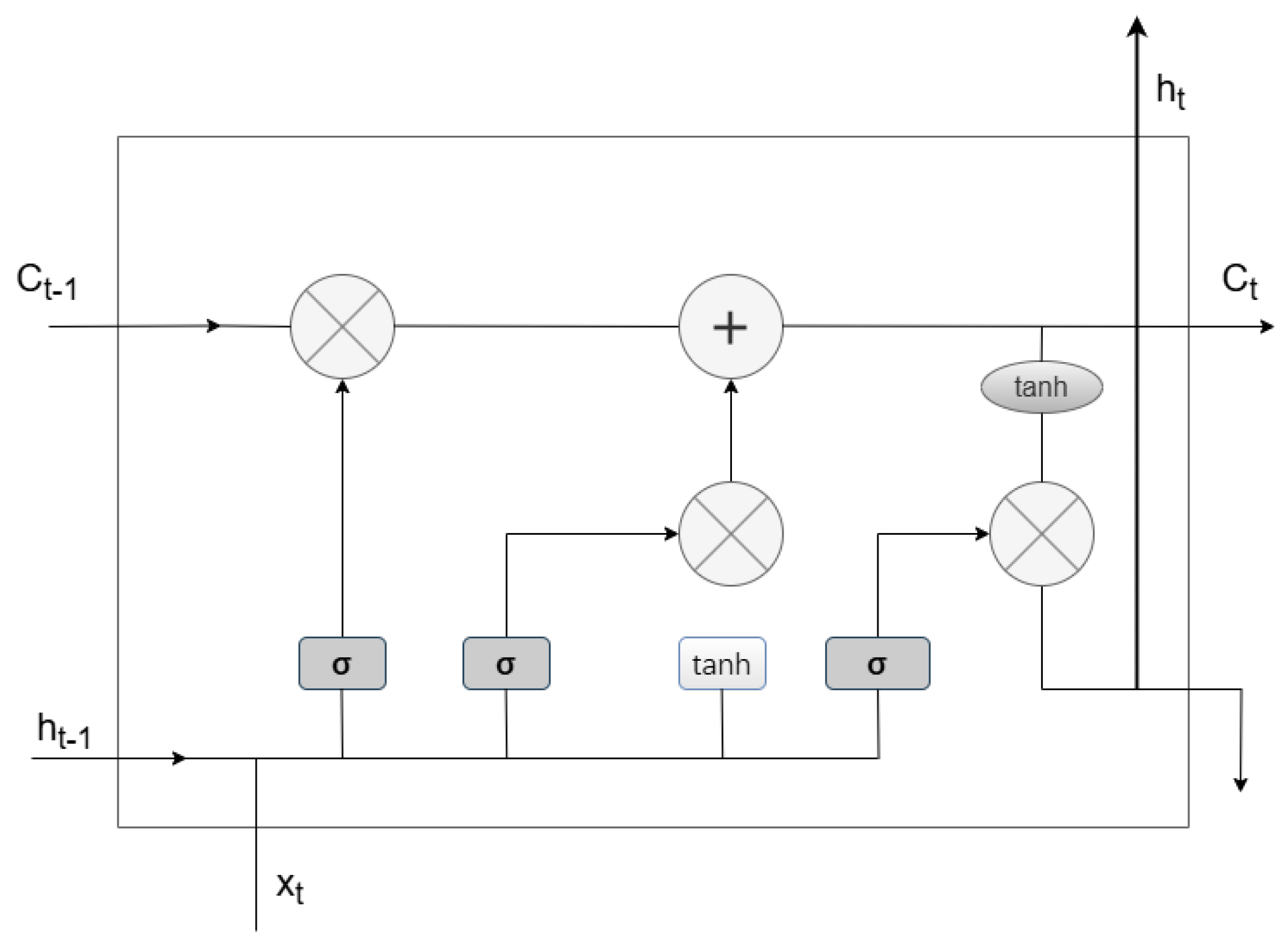
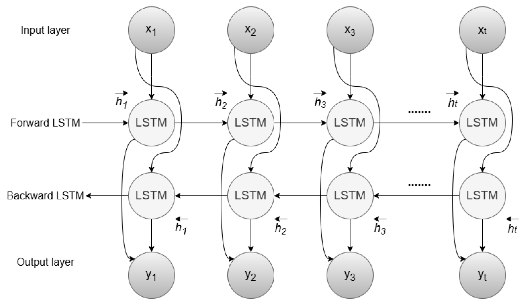
3.1.1. Bidirectional Long Short-Term Memory Neural Network (BILSTM) Model

Building electricity data has complex long-term dependencies. Long short-term memory neural network (LSTM) models are adept at using historical data for prediction but lack consideration of future information [10]. To deal with the characteristics of building electricity data, this study uses a bidirectional long short-term memory neural network (BILSTM) model as one of the base models. BILSTM is an improved recurrent neural network (RNN) composed of forward and backward double LSTM layers. It also incorporates past data and future information into model training to further improve the prediction accuracy compared to the unidirectional LSTM model [22].

There are three gates in the LSTM model architecture: the input gate, the output gate, and the forget gate [23]. The structure of an LSTM unit is shown in Figure 1. The forget gate determines the information that the cell needs to forget.

$$f_t=\sigma \left(W_f·[h_{t-1},x_t]+b_f\right)$$

(1)

The input gate is responsible for determining the data signal that needs to be output:

$$i_t=\sigma (W_i\times h_{t-1}+W_i\times x_i+b_i)$$

(2)

$${\tilde{C}}_t=tanh(W_c·[h_{t-1},x_t]+b_c)$$

(3)

$C_{t-1}$ is the old cell state, and the forgetting and input gates update it to $C_t$:

$$C_t=f_t\times C_{t-1}+i_t\times \widetilde{C_t}$$

(4)

The output gate determines the long-term state that needs to be output, and the neuron state that needs to be output is passed through the tanh layer and then multiplied by the activation function layer to obtain the output unit $h_t$ [10]:

$$o_t=\sigma (W_0·[h_{t-1},x_t]+b_o)$$

(5)

$$h_t=o_t\times tanh\left(C_t\right)$$

(6)

where $o_t$ is the output information, and $b_o$ is the deviation information.

The BILSTM unit structure is shown in Figure 2. At moment t, the forward LSTM computes the state of its own hidden layer as $\overrightarrow{h_t}$, the backward LSTM computes the state of its own hidden layer as $\overleftarrow{h_t}$, and the LSTM cell in the figure represents the computation process of the traditional LSTM model:

$$\overrightarrow{h_t}=LSTM(x_t,\overrightarrow{h_{t-1}})$$

(7)

$$\overline{h_t}=LSTM(x_t,\overline{h_{t-1}})$$

(8)

$$y_t=\sigma \left\{W_y·\left[\overrightarrow{h_t},\overline{h_t}\right]+b_y\right\}$$

(9)

$W_y$ denotes the weight and $b_y$ denotes the weight. In the structure diagram, $x_1$ to $x_t$ denotes the input information (i = 1, 2, 3, …, t) at each moment from $T_1$ moment until $T_i$ moment, and $y_1$ to $y_t$ denotes the output information (i = 1, 2, 3, …, t) at each moment from $T_1$ moment until $T_i$ moment.

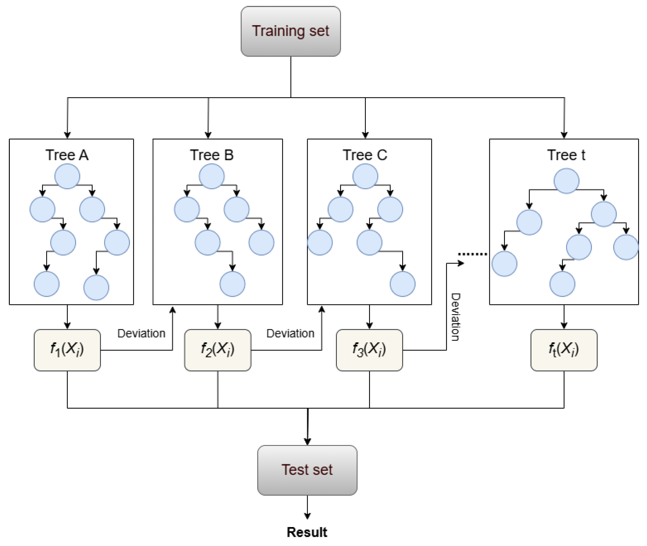
3.1.2. Random Forest (RF) Model

Random Forest (RF) is one of the Boosting algorithm models, which essentially integrates the weak learners to boost to strong learners. Random Forest uses the idea of random packing to take samples from the original dataset [24], constituting n new sample datasets, and then the data are processed using n different decision tree models respectively, and finally the final processing results are obtained after taking the average of these n decision tree models. The structure of the RF model algorithm is shown in Figure 3:

$$\widehat{y_i}={\displaystyle \frac{1}{N}}\Sigma \left(y_i\left(x\right)\right)$$

(10)

As in Equation (10), the final predicted value $\widehat{y_l}$ of the Random Forest is the average of the results of N decision trees, where x is the input sample, and $y_i\left(x\right)$ is the prediction result of each decision tree.

Random Forest integrates multiple decision trees following the principle of randomly selecting data samples as well as randomly selecting data features to make its prediction results more accurate and less prone to overfitting, which further improves the model’s generalization ability.

3.1.3. Extreme Gradient Boosting (XGBOOST) Model

XGBOOST is an ensemble learning algorithm based on Gradient Decision Trees (GBDTs) using the framework of gradient enhancement and is usually used for regression or classification tasks [25] as shown in Figure 4.

A number of different weak learners such as trees A, B, and C all the way up to tree t are stacked into one strong learner, and the prediction result of the strong learner is the sum of the results of the many weak learners. Equation (11) represents the tree from 1 to t, where each $f_k$ is a weak learner and $x_i$ represents the input information. Equations (12) and (13) represent the loss function and regularization term, respectively, where $y_i$ is the true value, $\widetilde{y_l}$ is the predicted value, T is the number of leaf nodes, $w_j$ is the weights of the leaf nodes, $\gamma$ is the decision tree complexity value, and $\lambda$ is the regularization parameter. XGBOOST is based on the greedy algorithm, which takes into account all the splitting points, and selects the feature with the smallest loss function at each step. XGBOOST has the ability to deal with the multiple feature input regression problem, and it performs in dealing with the high-dimensional data better, and the performance and stability of the model is also better [12]:

$$\widetilde{y_i}=\sum _{i=1}^t{f}_k\left(x_i\right)$$

(11)

$$(y_i,\widetilde{y_i})={(y_i-\widetilde{y_i})}^2$$

(12)

$$\Omega \left(f\right)=\gamma ·T+{\displaystyle \frac{1}{2}}\lambda ·\sum _{j=1}^T{w}_j^2$$

(13)

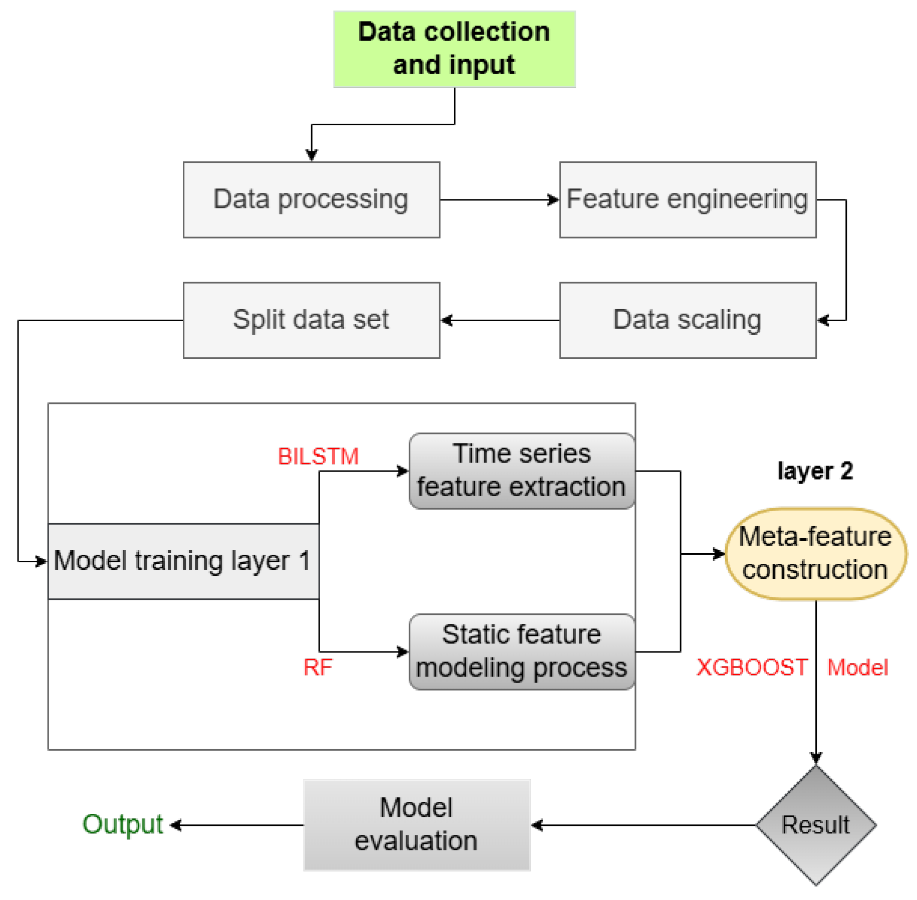
3.1.4. BILSTM-RF-XGBOOST Hybrid Model

This study proposes a novel hybrid model: the BILSTM+RF+XGBOOST model to improve the accuracy of electricity consumption prediction in buildings. The study adopts a two-layer stacked hybrid model structure, which is designed to fully consider the complex timing dependencies, nonlinear feature interactions, and potential noises in the electricity consumption data so as to significantly improve the robustness and accuracy of the model prediction.

Specifically, BILSTM and RF models are deployed in the first layer, which perform feature extraction and preliminary modeling of the input data from different dimensions. As the core functional part of time series extraction, the BILSTM model learns the dependence, periodicity, and consumption trend of power consumption in a long time series through its bi-directional structure, and uses the rich time series dynamics information as the feature vector training output.

The RF model is responsible for modeling static features and nonlinear relationships, and it focuses on mining original static features, time-derived features, and lagged features, and obtaining complex nonlinear mapping relationships between these input features and target variables. RF can effectively handle high-dimensional data by constructing multiple decision trees and integrating the results, capturing interactions between features, and providing good robustness to noise and outliers in the data. With good robustness, RF provides more robust prediction guarantees based on multiple decision trees while reducing the risk of overfitting, and can further simulate the feature interactions that are missed by BILSTM, reflecting the impact of static features on power consumption, making the output to the second layer more accurate and effective.

The study chooses to introduce both RF and BILSTM in the first layer, firstly due to the consideration of feature diversity and complementarity. In the context of the task of this study, due to the uniqueness of the electricity consumption behavior of different floors in that particular temperature interval, this trend of electricity consumption may not strictly follow the temporal pattern, and the ability of RF to capture such patterns is better than the purely temporal model BILSTM, so the work of dynamic temporal feature extraction and nonlinear static feature modeling can work together to provide the meta-learner with a more comprehensive and diversified perspective of information. Second, since one of the core ideas of stacked integration is to improve the overall performance through diversity, two base models with completely different mechanisms and focuses can better enrich the input features of the meta-learner. The fundamental reason for choosing XGBOOST as the meta-learner in stacked integration is that the model has high efficiency, high accuracy, and good generalization ability, which not only can effectively handle inputs from multiple base models but also can minimize the risk of overfitting to a certain extent as follows.

In the second layer, the XGBOOST model is used as a meta-learner, which uses a stacking mechanism to combine the two set-based models in the first layer to form a meta-feature vector, which is then used as an input feature [26] and trained using the XGBOOST model. As a meta-learner, the goal of XGBOOST is to weigh and combine the optimal prediction information from the two models in the previous layer so as to generate highly accurate prediction results that ultimately fuse the temporal and static features. The implementation of this study is shown in Figure 5.

3.2. Bayesian Optimization Algorithm Under K-Fold Cross-Validation

The Bayesian algorithm is an efficient global optimization method based on a surrogate model and an acquisition function. Its fast convergence to an optimal value is the main reason for its wide application in the process of model-based optimal hyperparameter selection [27]. The model algorithm adopted in this study faces the challenge of a large number of hyperparameters with high complexity in hyperparameter selection. Traditional grid search or random search of hyperparameters will encounter problems of high computational cost and long running time [28]. The core advantage of the Bayesian algorithm is to use the prior mechanism, combined with the historical hyperparameter evaluation results, and then use the surrogate model to guide the subsequent search range, quickly and accurately improve the optimal hyperparameter combination obtained, and reduce the running cost of the model. The hyperparameter combination improved by the Bayesian algorithm often maximizes model performance.

To ensure the effectiveness of the Bayesian optimization process and also to ensure that the model reduces the risk of overfitting, a 5-fold time series cross-validation is integrated in this study. First, the original dataset is chronologically divided into a training set (first 70%), an initial validation set (10%) and a final test set (last 20%). In the Bayesian optimization stage, this study merges the training set with the initial validation set (80% of the total data), and next, for the merged training set and initial validation set, it is divided into five folds, and in each fold, the earlier data are used as the training data for the cross-validation (CV-train), and the immediately following data blocks are used as the validation data for the cross-validation (CV-validation). Finally, for each set of hyperparameters, each model will be trained on each of the five CV-train sets and the R2 metric performance will be evaluated on the pairwise used five CV-train sets. Whereas the objective of Bayesian optimization is to maximize the average of the performance metrics on these 5 CV-validation sets, the approach taken in this study makes the selection of hyperparameters insensitive to a single validation segmentation, which enhances the robustness of the selected hyperparameters.

Also, this study predefines explicit search space boundaries for the hyperparameters to be optimized for each prediction model. These boundaries frame the range of parameter combinations explored by the optimizer, and the detailed information is shown in

Table 1. Bayesian optimization hyperparameter search space boundaries.

Model/Component	Hyperparameter	Search Range	Remarks
Base Models (RNN, LSTM, BiLSTM)
RNN	units	(32, 128)	Number of RNN units
	dropout_rate	(0.0, 0.5)	Dropout rate
	learning_rate	(0.0001, 0.01)	Learning rate
LSTM	units	(32, 128)	Number of LSTM units
	dropout_rate	(0.0, 0.5)	Dropout rate
	learning_rate	(0.0001, 0.01)	Learning rate
BiLSTM	units	(32, 128)	Units per LSTM in BiLSTM
	dropout_rate	(0.0, 0.5)	Dropout rate
	learning_rate	(0.0001, 0.01)	Learning rate
	seq_length	(5, 20)	Input sequence length
XGBoost (Base Model and Meta-Learner Component)
XGBoost	n_estimators	(100, 1000)	Number of trees
	learning_rate	(0.005, 0.1)	Learning rate
	max_depth	(3, 10)	Tree max depth
	subsample	(0.6, 1.0)	Subsample ratio of training samples
	colsample_bytree	(0.5, 1.0)	Subsample ratio of columns
	gamma	(0.0, 0.5)	Minimum loss reduction for split
	reg_alpha	(0.0, 0.5)	L1 regularization
	reg_lambda	(0.0, 0.5)	L2 regularization
BiLSTM-XGBoost (Hybrid Model)
BiLSTM component	lstm_units	(32, 128)	BiLSTM units
	lstm_dropout_rate	(0.0, 0.5)	BiLSTM dropout rate
	lstm_learning_rate	(0.0001, 0.01)	BiLSTM learning rate
XGBoost component	n_estimators	(100, 1000)	XGBoost trees
	learning_rate	(0.005, 0.1)	XGBoost learning rate
	max_depth	(3, 10)	XGBoost tree depth
	subsample	(0.6, 1.0)	XGBoost subsample
	colsample_bytree	(0.5, 1.0)	XGBoost column subsample
	gamma	(0.0, 0.5)	XGBoost gamma
	reg_alpha	(0.0, 0.5)	XGBoost L1 regularization
	reg_lambda	(0.0, 0.5)	XGBoost L2 regularization
BiLSTM-RF-XGBoost (Hybrid Model)
BiLSTM component	lstm_units	(32, 64)	BiLSTM units
	lstm_dropout_rate	(0.1, 0.4)	BiLSTM dropout rate
	lstm_learning_rate	(0.001, 0.01)	BiLSTM learning rate
RF component	n_estimators_rf	(50, 300)	RF number of trees
	max_features	(0.6, 0.9)	RF max features ratio
	min_samples_leaf	(3, 15)	RF minimum samples per leaf
XGBoost component	n_estimators_xgb	(100, 500)	XGBoost number of trees
	learning_rate_xgb	(0.01, 0.1)	XGBoost learning rate
	max_depth_xgb	(3, 8)	XGBoost tree depth
	subsample_xgb	(0.6, 0.9)	XGBoost subsample ratio
	colsample_bytree_xgb	(0.5, 0.9)	XGBoost column subsample
	gamma_xgb	(0.1, 0.6)	XGBoost gamma
	reg_alpha_xgb	(0.1, 0.6)	XGBoost L1 regularization
	reg_lambda_xgb	(0.1, 0.6)	XGBoost L2 regularization

. Within these defined search spaces, the Bayesian optimization process consists of 5 initial random exploration points and 15 subsequent iterations of optimization, for a total of 20 evaluations of the hyperparameter combinations for each model.

3.2.1. Gaussian Process (GP) Surrogate Model

Although the inputs can be defined during the research process, the hyperparameter indicators are obtained by training and evaluating the BILSTM-RF-XGBOOST model, but this complex process is not visible. The relationship between hyperparameters and the final model performance not only depends on the hyperparameters themselves, but also on the training and validation sets and the randomness within the model. When we try to improve the hyperparameters to make them an optimal solution for model performance, this required goal is equivalent to optimizing a black box function. Complex hybrid models result in high computational costs for the optimization of this black box function. Bayesian algorithms reduce these costs while improving the effectiveness of hyperparameter improvement by defining computationally cheap surrogate models to approximate the true but unknown objective function.

In this study, the Gaussian process (GP) is used by default for the Bayesian optimization process as a proxy model for the Bayesian optimization algorithm. This is because we used the default configuration of the bayes_opt library, i.e., Matern 2.5 kernel function. This study explicitly defines kind = “ei” during BayesianOptimization initialization, i.e., Expected Improvement (EI) is used as the acquisition function. The Gaussian process is a flexible non-parametric probabilistic model that can model the mapping function of various hyperparameter combinations to model performance in this study, which is important for the integrity of the Bayesian optimization framework [14].

The core idea of the GP is to define a target function that approximates a prior distribution defined by a mean function and a covariance function without any observational data as in Equation [28]:

$$f\sim N\left(m\left(X\right),K(X,X)\right)$$

(14)

where f is the objective function, $N\left(m\left(X\right),K(X,X)\right)$ represents a Gaussian distribution with mean $m\left(X\right)$ and covariance matrix $K(X,X)$, where the covariance matrix is also called the kernel matrix, and its element $K_{ij}=k(x_i,y_j)$ is calculated by the kernel function $k(x,x^{\prime })$. The choice of the kernel function results in an approximation of the assumptions made about the objective function. The radial basis function kernel is widely used in Bayesian algorithms and is also called the Gaussian kernel as shown in Equation (15):

$$k(x,x^{\prime })={\sigma }^{2}exp\left(-{\displaystyle \frac{{∥x-x^{\prime }∥}^2}{2l^2}}\right)$$

(15)

Among them, the signal variance ${\sigma }^2$ controls the range of changes in the function value. $\parallel x-x^{\prime }{\parallel }^2$ measures the distance between two input points in the feature space. The Gaussian kernel proposes that points with similar distances in the hyperparameter space tend to have similar model performance. Given the existing observations $D={\left\{(x_i,y_i)\right\}}_{\mathrm{i}=1}^n$, where $y_i=f\left(x_i\right)+{\epsilon }_i,{\epsilon }_i\sim N(0,{\sigma }_n^2)$ is the observation noise. The Gaussian process updates the prior distribution using Bayes’ theorem so that the posterior distribution of the objective function at an unknown point still conforms to a Gaussian distribution where $u\left(x_{*}\right)$ is the posterior mean and ${\sigma }^2\left(x_{*}\right)$ is the posterior variance:

$$f\left(x_{*}\right)\sim N\left(u\left(x_{*}\right),{\sigma }^2\left(x_{*}\right)\right)$$

(16)

The GP prediction is more accurate near existing observation points, and the a posteriori variance is smaller. Conversely, the GP prediction in unobserved areas is more uncertain, which leads to a larger a posteriori variance. As a non-parametric probability model, the GP has the flexibility to fit the form of complex objective functions. The a posteriori variance of the uncertainty in the prediction is quantified and provided to the Bayesian algorithm as the search strategy for subsequent improvement of the expected function.

3.2.2. Expected Improvement (EI) Collection Function

The role of the Expected Improvement Acquisition (EI) function is to guide the Bayesian optimization algorithm in selecting the next point to be evaluated, and the EI value gives the next prediction suggestion based on the predicted mean as well as the variance of the GP, and tends to select the regions with higher mean values, which represent potential hyperparameter combinations with better performance. Regions with higher variance are chosen because they represent insufficient exploration of the model, and better solutions may exist in these unknown regions [28].

The Bayesian optimization algorithm is an iterative optimization method that iteratively maximizes the EI acquisition function, selects the next evaluation point, and continuously updates the Gaussian process agent model to ultimately find a globally optimal or near-globally optimal solution of the objective function within a finite number of iterations [14]. The goal of the desired improvement of the acquisition function is to maximize the improvement of the objective function value $f\left(x\right)$ at the next evaluation point x compared to the current optimal value $y_{best}$, as in Equation (17), where $y_{best}$ is the optimal objective function value. When assuming that $y_{best}$ is known and that the function value $f\left(x\right)$ at point x conforms to a Gaussian distribution, the Expected Improvement Acquisition (EI) function is formulated as in Equation (18) where $\Phi \left(z\left(x\right)\right)$ is the cumulative distribution function of the standard state distribution, and $\varphi \left(z\right(x\left)\right)$ is the probability density function of the standard state distribution. $u\left(x\right)$ and $\sigma \left(x\right)$ make the posterior mean and posterior standard deviation, respectively, of the predictions of the Gaussian process agent model:

$$EI\left(x\right)=E\left[\max (0,f\left(x\right)-y_{best})\right]$$

(17)

In Equation (17), a larger value of $EI\left(x\right)$ indicates a greater expectation of sampling at point x and obtaining a better result than the current optimal objective function value $y_{best}$:

$$EI\left(x\right)=\sigma \left(x\right)\left[z\left(x\right)\Phi \left(z\left(x\right)\right)+\varphi \left(z\left(x\right)\right)\right]$$

(18)

$$z\left(x\right)={\displaystyle \frac{u\left(x\right)-y_{best}}{\sigma \left(x\right)}}$$

(19)

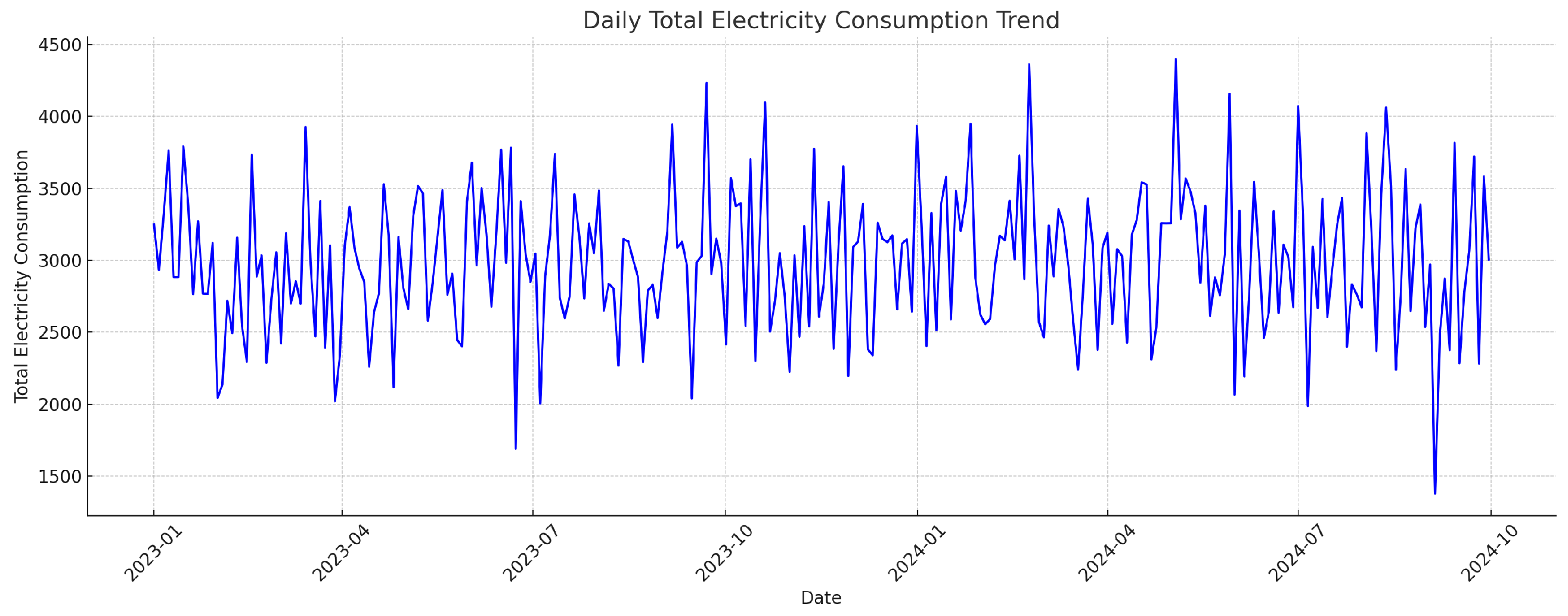
3.3. Data Collection and Pre-Processing

To ensure that the stacked mixed model proposed in this study provides a more realistic and reliable prediction of building electricity consumption, this study uses actual electricity consumption data from the real world. The following section details the source and collection of the experimental data and the data processing implemented to meet the model input requirements and improve data quality, with the aim of laying a solid and reliable data foundation for model construction and result analysis.

3.3.1. Data Sources and Pre-Processing

The source of the dataset used in this study is the power consumption data of the T8 building in the smart energy system developed by the project partner company—Shanghai Pudong Taopu Company, which is read and stored in the local server by means of an API interface. The dataset used in this study covers the power consumption data of this building from 1 to 25 floors during the period from 1 January 2023 to 30 September 2024, with a total size of 15,975 data, and the time resolution of the data collection is once a day, with power data of 25 floors per day. The data was collected through the company’s building automation system to ensure the authenticity and reliability of the data. The building’s power consumption is affected by a combination of factors, which are mainly considered in this paper, such as the ambient temperature in which the building is located, the different floors in the building structure, and the weekday holidays. The dataset contains key fields as shown in

Table 2. Table 1 Key fields in the data.

Field Name	Data Type	Description
data	Datetime	Date
electricity_consumption	Numerical	Daily total electricity consumption
temperature	Numerical	Daily average temperature
is_holiday	Boolean	Whether the day is a holiday
Seasonality_Features	Categorical	reflecting weekly seasonality

.

The original dataset needs to undergo a strict and effective pre-processing process to improve the data quality and ensure the effectiveness and accuracy of the model training before it is applied to the model training. In the data processing stage, the outliers are first eliminated to prevent the interference of abnormal data on the model training, and then the data are examined, and a small number of missing values due to the lagging operation in the feature engineering are found. For these missing values, a zero-filling strategy is used. This strategy is chosen because the percentage of missing values is small and zero-filling has a relatively small impact on the overall data distribution and model learning. Then the date format is converted from string to datetime, which is convenient for time series analysis and feature extraction.

Then, this paper adopts the method of Min-Max Scaling to normalize the numerical features, and scales the data to the range of [0, 1] interval to accelerate the convergence of model training [22]. For categorical features, such as floor floors as well as Seasonality_Features weekly seasonal features, a solo thermal coding technique is used to convert them into dummy variables so that the machine learning model can handle the data. Finally, in order to ensure the continuity of the time series data as well as the consistency of the order of the floors, the data are sorted according to the DATA field. In fact, during the data collection phase, this study already organized the data in order, but in order to ensure the rigorous accuracy of the study, the sorting work is performed again. Meanwhile, in order to carry out effective model training, hyperparameter optimization, and performance evaluation, this study adopts the temporal order segmentation method to divide the dataset into a training set, validation set, and test set. In this study, 70% of the dataset is selected as the training set to train the model (from 1 January 2023, to 22 March 2024), 10% as the validation set for hyperparameter tuning and model selection (from 23 March 2024, to 25 May 2024), and finally 20% as an independent test set. The performance of the final selected model is evaluated and the generalization capability indicator is obtained (from 26 May 2024, to 30 September 2024). Since the data of the test set is completely invisible in the model training and parameter adjustment stage, this practice is an important means to ensure the effectiveness of model evaluation. It can simulate the predictive performance of the model in real conditions so that the model cannot contact future data in the training stage and only evaluates its predictive ability of future data on the verification set and test set, thus avoiding data leakage. It more truly reflects the generalization of the model. The total daily power consumption on all floors of the building in the raw data is shown in Figure 6.

3.3.2. Feature Engineering

Electricity data contains multi-scale and multi-dimensional information, and effective feature engineering can make the model more accurate for training and learning of electricity consumption prediction [4]. In this study, the autocorrelation of time series is utilized to construct lagged features, specifically, the 1st-, 2nd-, 3rd-, and 7th-order lagged features are selected to represent the power consumption and temperature information of the previous 1, 2, 3, and 7 days, respectively, and the lagged features can help the model to better capture the impact of historical information on the current stage of power consumption. In addition, in order to learn the long-term seasonal and short-term cyclical fluctuations in power consumption, the data date field data is derived to extract the annual scale, quarterly scale, monthly scale, and daily scale temporal features. It should be noted that the annual scale temporal features may make the model mistakenly think that the 365th day and the 1st day are numerically “very far away” if the day of year (1 to 365) is used, while in fact they are adjacent to each other in the annual cycle. So in this study, in order to help the model more accurately capture the annual periodicity law and solve the cyclic continuity problem of this temporal feature, it is studied that the day of year is transformed by the sine and cosine functions so that the values of the end of the year and the beginning of the year in the transformed space are continuous to help the model learn the cyclic fluctuation patterns at different time granularities and provide more accurate forecasting results.

4. Experimental Setup and Analysis of Results

4.1. Model Evaluation Criteria

In this study, a variety of common time series forecasting evaluation metrics (all evaluation metrics are completed by calculating the forecasts of the model’s test set) are used, namely, the Mean Squared Error MSE (Mean Squared Error), the Root Mean Squared Error RMSE (Root Mean Squared Error), the Mean Absolute Error MAE (Mean Absolute Error), Mean Absolute Percentage Error (MAPE), and the coefficient of determination R² (R-squared), where RMSE is the root of MSE [23]. These four evaluation indexes can observe the accuracy of the model prediction results and the excellence of the model fit from different perspectives, providing strong support for the research. As shown in Equation (20) to Equation (23) below, where $\widehat{y_i}$ denotes the model predicted value of the ith sample, $y_i$ denotes the true value of the ith sample, and N is the total number of samples. In the evaluation indexes, the ranges of the MSE value, RMSE value, MAPE value, and MAE value are all $[0,+\infty )$. The smaller the value, the higher the prediction precision of the model and the higher the accuracy. As in Equation (24), the coefficient of determination R² typically ranges between 0 and 1 when evaluated on training data. However, when evaluated on an independent test set, R² may be negative if the model performs inferiorly to a benchmark predictor (e.g., predicting the average of the training data), which is not a rigorous approach for academic research. In this study, although the average R² value using K-fold time series cross-validation (TSCV R²) is chosen to guide hyperparameter optimization, the main metrics used to evaluate the performance of the final model on an independent test set are MSE, root mean square RMSE, MAE, and MAPE, due to the fact that they are the only evaluative metrics that directly quantify the prediction error:

$$MSE={\displaystyle \frac{1}{\mathrm{N}}}\sum _{i=1}^{\mathrm{N}}{(y_i-{\widehat{y}}_l)}^2$$

(20)

$$RMSE=\sqrt{{\displaystyle \frac{1}{N}}{\displaystyle \sum _{i=1}^N}{(y_i-{\widehat{y}}_l)}^2}$$

(21)

$$MAE={\displaystyle \frac{1}{\mathrm{N}}}{\Sigma }_{i=1}^{\mathrm{N}}|y_i-{\widehat{y}}_l|$$

(22)

$$MAPE={\displaystyle \frac{1}{N}}\sum _{i=1}^N\left|{\displaystyle \frac{y_i-{\widehat{y}}_i}{y_i}}\right|\times 100\%$$

(23)

$$R^2=1-{\displaystyle \frac{{\Sigma }_{\mathrm{i}=1}^n{(y_i-\widehat{y_l})}^2}{{\Sigma }_{\mathrm{i}=1}^n{(y_i-\overline{y})}^2}}$$

(24)

4.2. Optimal Hyperparameter Setting

In order to overcome the blindness and inefficiency of traditional manual hyperparameter tuning and to effectively prevent model overfitting, this study introduces rigorous K-fold time series cross-validation in the Bayesian optimization process to screen the optimal hyperparameter configurations for each model, which are obtained after optimizing the average performance of TSCV. The core of Bayesian optimization lies in iteratively searching for the optimal parameter combinations based on the performance on the validation set, and selecting hyperparameters that maximize the generalization capability by continuously evaluating the model’s performance on the validation set so as to avoid the model overfitting the training data. For traditional neural network models (RNN, LSTM, BILSTM), Bayesian optimization mainly adjusts the units, dropout rate and learning rate, in which the reasonable setting of the dropout layer can effectively avoid the phenomenon of neural network model overfitting. For the hyperparameter optimization of the XGBOOST model, a higher number of trees and tree depth allow the model to build deeper and more complex tree integrations to capture the complex relationships in the data. A moderate learning rate is used to balance the speed of model learning and the stability of model convergence.

The Bayesian optimization results of this study for each model hyperparameter are shown in

Table 3. Optimal hyperparameters for all evaluated models.

Name	RNN	LSTM	BILSTM	XGBOOST	BILSTM-XGB	BILSTM-RF-XGB
units	68	95	125	\	64 (BILSTM)	116 (BILSTM)
dropout_rate	0.024	0.001	0.030	\	0.094 (BILSTM)	0.1 (BILSTM)
learning_rate	0.009	0.010	0.007	\	0.010 (BILSTM)	0.002 (BILSTM)
seq_length	5	5	5	\	\	\
n_estimators	\	\	\	912	217	114
XGB learning_rate	\	\	\	0.050	0.080	0.066
max_depth	\	\	\	11	7	4
subsample	\	\	\	0.864	0.618	0.936
colsample_bytree	\	\	\	0.567	0.761	0.867
gamma	\	\	\	0.011	0.008	0.015
reg_alpha	\	\	\	0.030	0.023	0.092
reg_lambda	\	\	\	0.165	0.140	0.175
RF max_features	\	\	\	\	\	0.855
RF min_samples_leaf	\	\	\	\	\	3
RF n_estimators	\	\	\	\	\	350

, and some hyperparameters that must be integers in the actual implementation of the model training were rounded up. By comparison, it is easy to find that the optimal BILSTM hyperparameter configuration for the BILSTM -RF-XGBOOST model tends to have a higher number of cells and stronger regularization (higher Dropout ratio), while adopting a more conservative learning strategy (smaller learning rate). This implies that in more complex stacked structures, BILSTM needs to take on heavier feature extraction tasks and requires finer hyperparameters to avoid overfitting. Whereas in the XGBOOST meta-learner focuses more on a high number of, shallower depth tree structures, focusing on fusing the predictions of the base model rather than constructing overly complex decision trees.

In addition, it is worth noting that the Early Stopping early stopping mechanism is also used in this study during the training process of the neural network model. This mechanism terminates the training early by determining that the loss function does not decrease within a specified number of epochs, and restores the model weights to the number of epochs when the performance on the validation set, in order to further improve the model’s generalization ability and prevent the overfitting phenomenon during the training process.

The analytical results of the optimal hyperparameter table reveal the learning mechanism of the model while corroborating the complexity of stacked model design and tuning. The complexity of the BILSTM + RF + XGBOOST model proposed in this study is high, and both its base model and meta-learner require finer parameter configurations to achieve optimal performance. Bayesian optimization in automatically searching and determining the optimal hyperparameter combinations for these complex models achieves a model that can pursue high accuracy while effectively preventing overfitting and reflecting good generalization ability.

In addition, it is worth noting that this study also uses an early stopping mechanism during the training of the neural network model. This mechanism terminates the training early by judging that the loss function has not decreased within a specified number of epochs, and restores the model weights to the epoch number when the validation set performance is the best, in order to further enhance the generalization ability of the model and prevent overfitting during training.

The analysis results of the optimal hyperparameter table not only confirm the complexity of stacked model design and tuning but also reveal the learning mechanism of the model. The BILSTM + RF + XGBOOST model proposed in this study is highly complex, and both its base model and meta-learner require more refined parameter configurations to achieve optimal performance. Bayesian optimization automatically searches for and determines the optimal combination of hyperparameters for these complex models, enabling the model to pursue high accuracy while also effectively preventing overfitting and demonstrating good generalization ability.

4.3. Experimental Results and Analysis

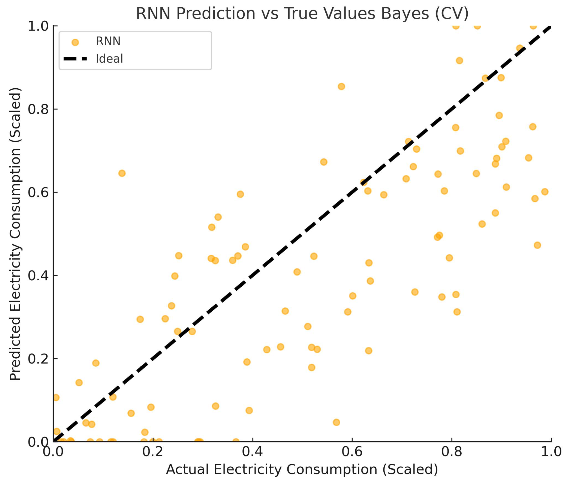
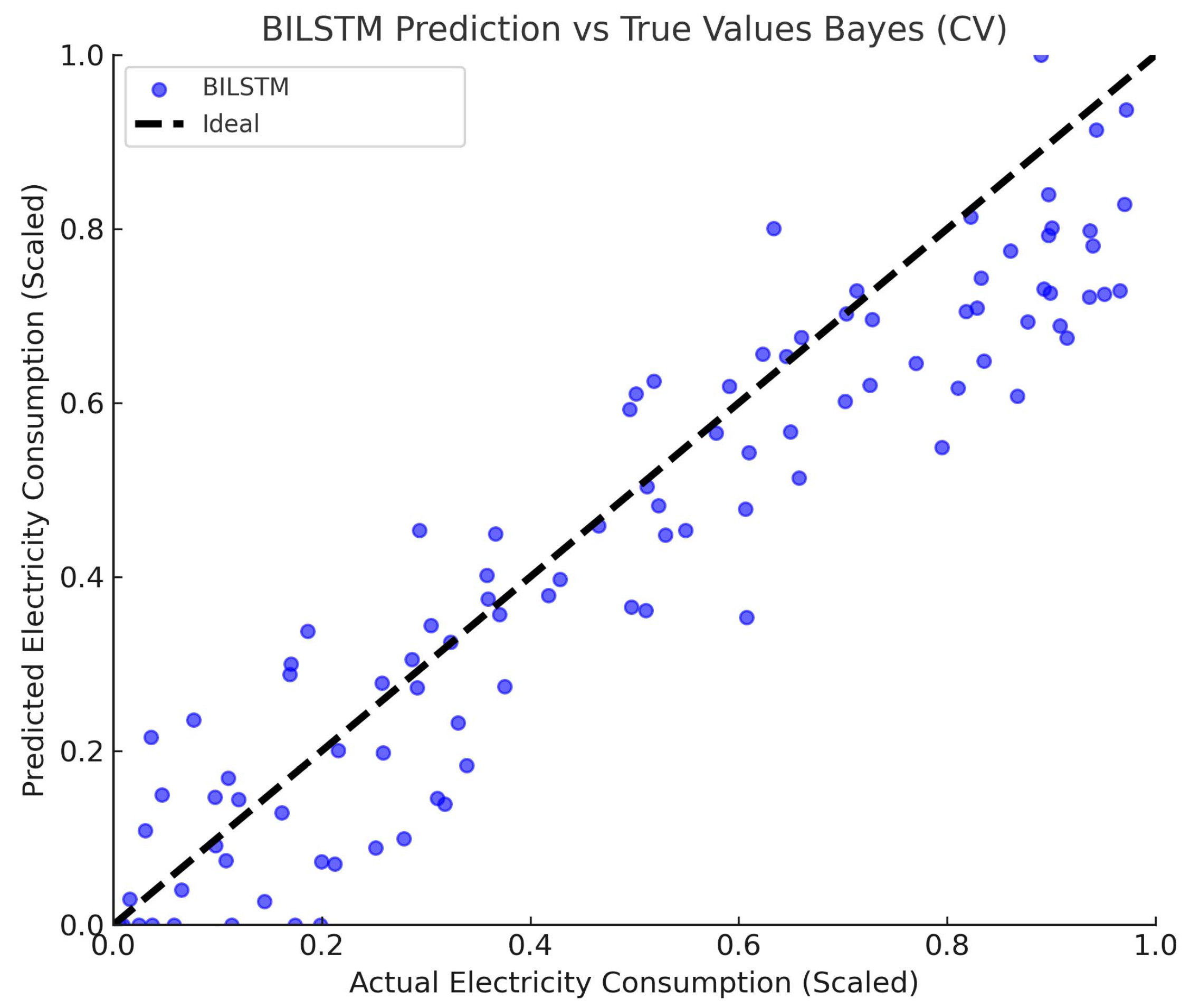
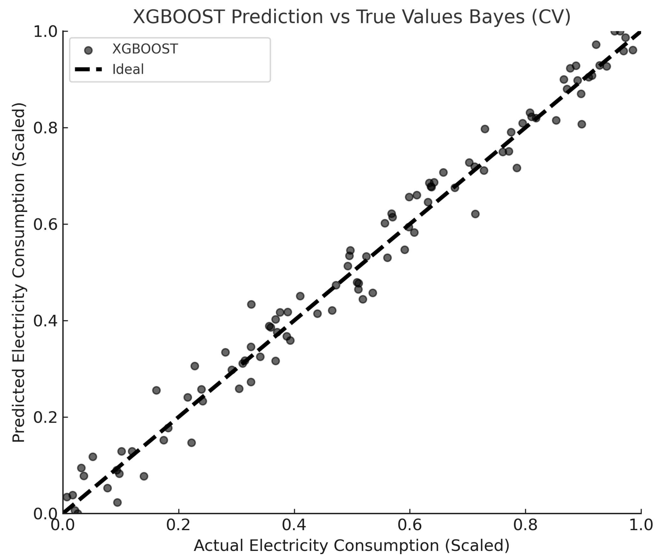
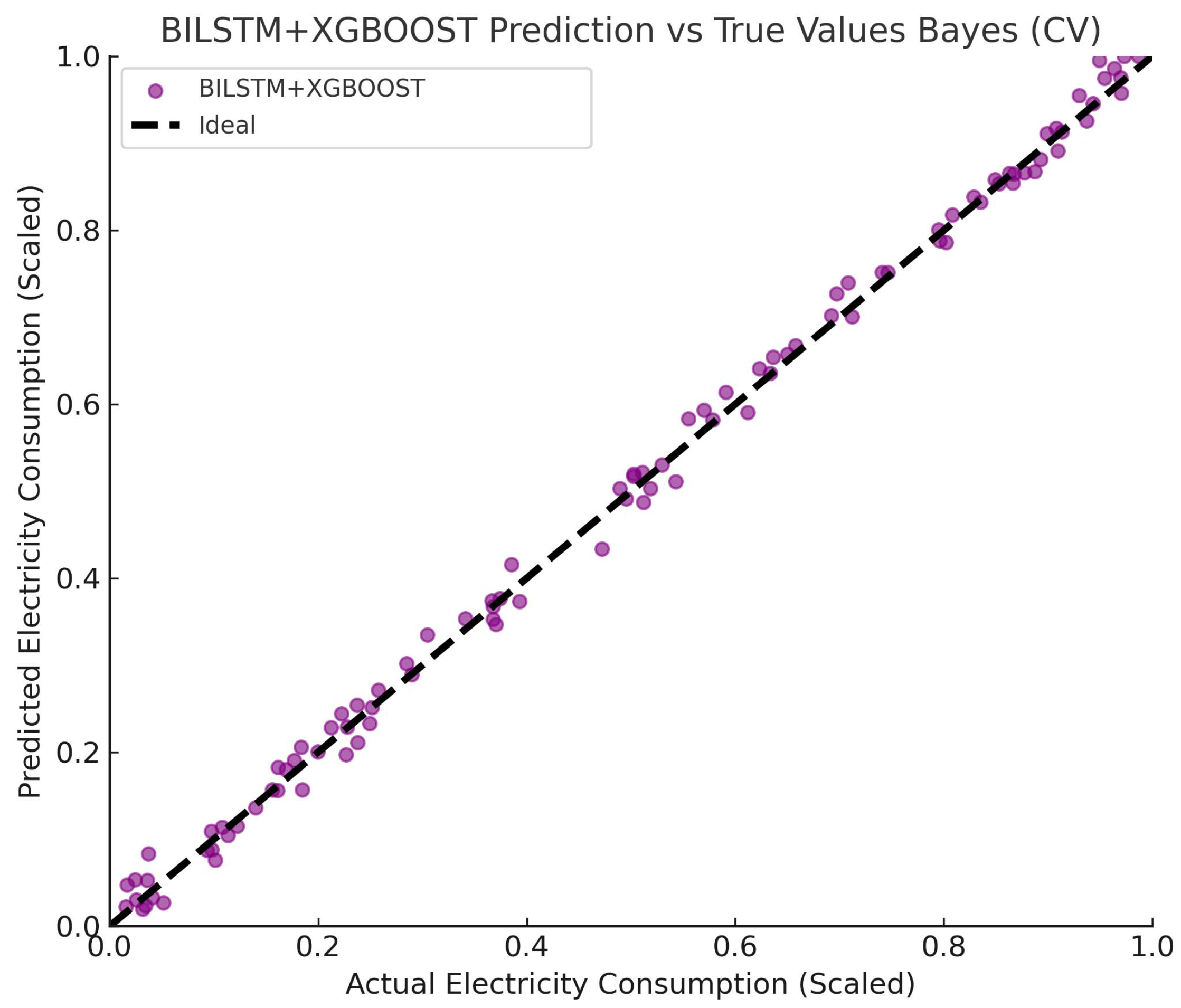
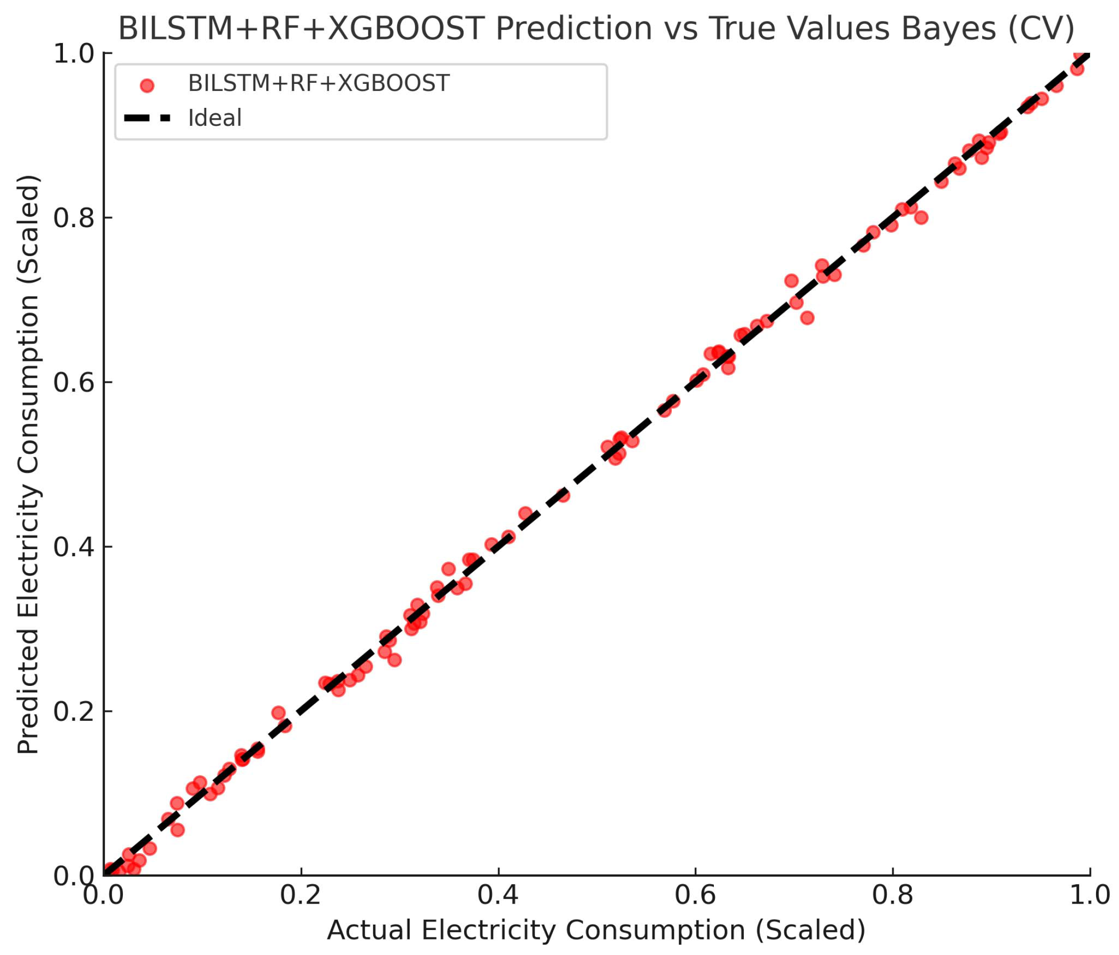
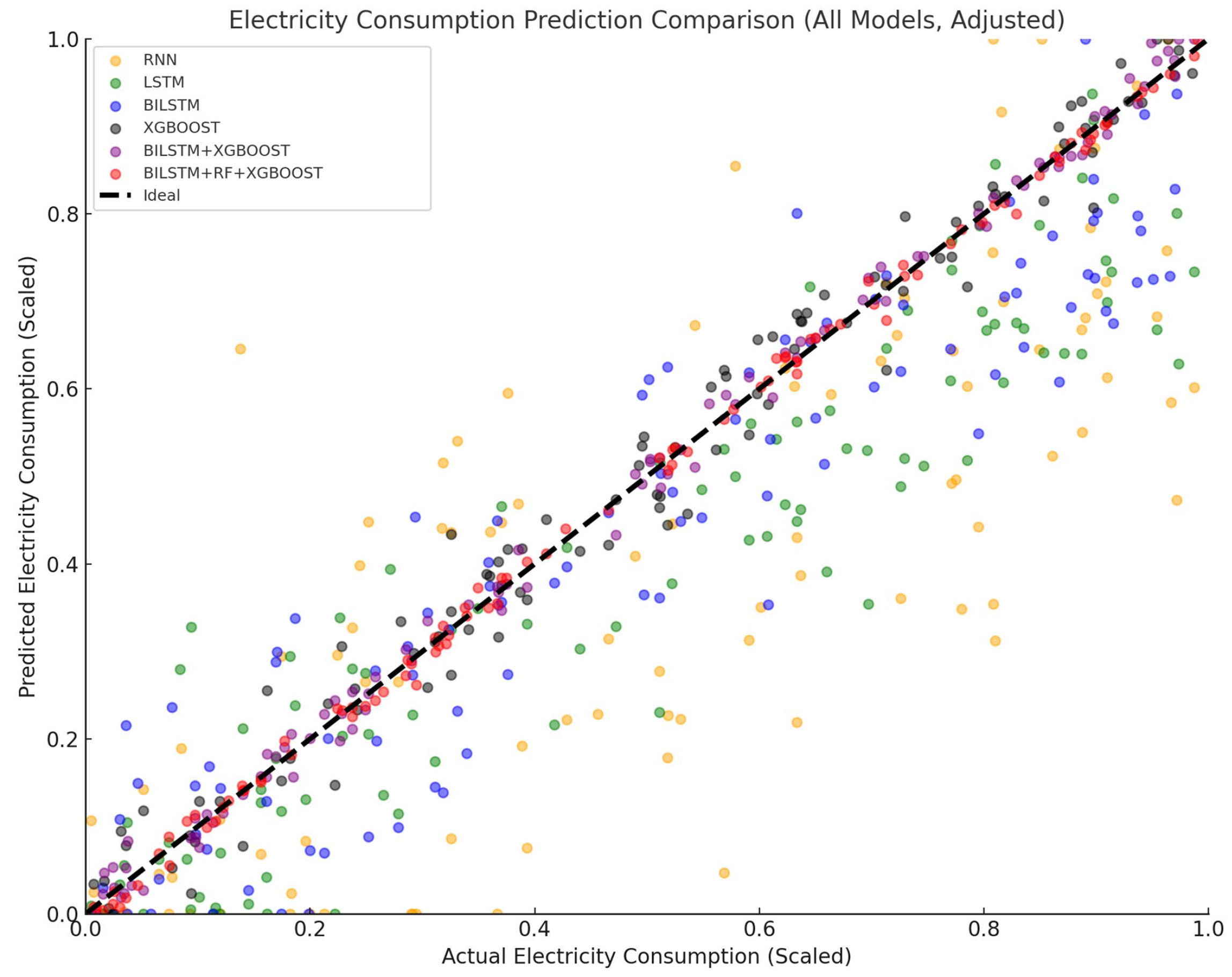
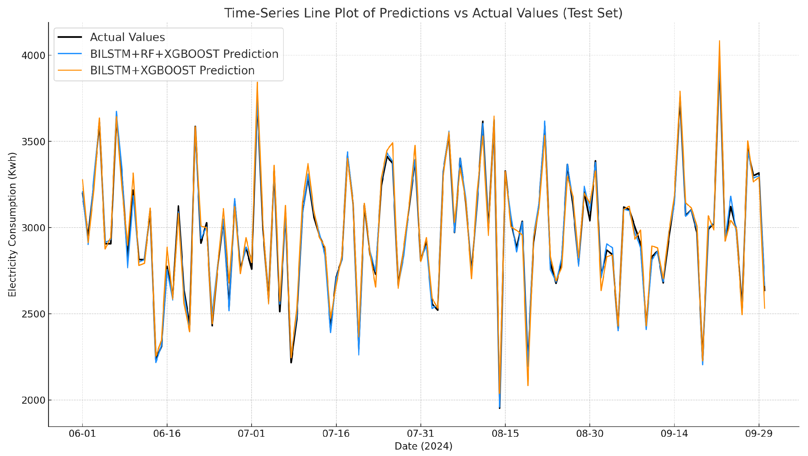
4.3.1. Analysis of Projected Results

In this section, we will delve into the prediction results of the BILSTM+RF+XGBOOST stacked hybrid and comparison models (including RNN, LSTM, BILSTM, XGBOOST, and the BILSTM+XGBOOST hybrid model) trained based on an independent test set. To ensure the rigor of the study, all model hyperparameters are screened by a Bayesian optimization algorithm incorporating K-fold time series cross-validation. The prediction results of each model are shown in Figure 7, Figure 8, Figure 9, Figure 10, Figure 11, Figure 12 and Figure 13. In order to intuitively assess the good or bad performance of the models in building electricity prediction, this study adopts the scatterplot of predicted and real values of electricity consumption normalized by Min–Max values in the range of [0, 1] for visualization and analysis. Due to the large range of raw electricity consumption values, without normalization, the experimental results will have problems such as excessive differences in data points and loss of detailed information for smaller variables due to compression. These problems will make it impossible for researchers to observe the subtle differences between data points as well as the distribution patterns, and will also make the graphs difficult to interpret, losing the essential purpose of visualization to convey information. Finally, it should be emphasized that the standardized visual graph analysis does not appear to have any impact on assessing the predictive performance of the model and still reflects the accuracy and degree of bias of the model prediction.

As can be seen in Figure 7, the RNN model has the worst performance results, and the traditional recurrent neural network has serious bias problems when facing this kind of complex multi-dimensional time series prediction task, and hardly affixes to the ideal diagonal scatter distribution, which indicates that the RNN is unable to effectively learn the complex structure of the electricity consumption data of the building, and also is unable to efficiently capture the long-distance dependency relationship. Figure 8 shows the prediction results of the LSTM model, although it has been slightly improved relative to the RNN, but its prediction points still have a haphazard distribution phenomenon. This illustrates the inadequacy of the limited ability of LSTM to learn temporal features and its inability to adequately model the data.

The prediction results of BILSTM are given in Figure 9, and it is found that its prediction values are also highly scattered. Especially in the middle and high value regions, the predicted values are extremely different from the true values. Theoretically, BILSTM can capture bidirectional information for better training results, but its performance cannot be fully utilized in the current task environment. Figure 10 uses a single XGBOOST model for training, and the prediction result set of this single model is supposed to be distributed along the ideal diagonal but still shows large errors in some prediction points, which may be caused by the lack of learning ability of certain temporal features.

Figure 11 uses the hybrid model of BILSTM+XGBOOST. The results are closer to the ideal value, and the degree of dispersion is further reduced, but there are still a small number of prediction points that deviate from the ideal value diagonal, which indicates that although the XGBOOST and BILSTM models are able to correct some of the errors of the other model to a certain extent, it is not enough to completely compensate for the repair, and there is a possibility of higher improvement in the accuracy of the prediction results.

Finally, Figure 12 shows the prediction results of the stacked hybrid model BILSTM+RF+XGBOOST proposed in this study. The prediction results are almost perfectly adhered to the diagonal of the ideal value, and there is almost no obvious deviation from the scattering point, which indicates that the model has a very high fitting ability and very small prediction bias, and it also proves that the hybrid model proposed in this study has a strong generalization ability. Figure 13 shows the comparison of the prediction results of all models, from which it is not difficult to see the excellence and accuracy of the prediction results of the BILSTM-RF-XGBOOST model proposed in this study. Next, the evaluation indicators of all models are compared and analyzed.

In order to better evaluate the performance of the models in time series forecasting, line plots of the predicted and actual values are added to the key models in the study (BILSTM-XGBOOST and BILSTM-RF-XGBOOST) as shown in Figure 14, which clearly demonstrate the performance of the BILSTM-RF-XGBOOST model proposed in this study, and proves that not only is it able to precisely capture the overall trend and cyclical fluctuations of power consumption but also shows better performance in detail fitting, peak and valley value prediction, and response to sudden change points compared to BILSTM-XGBOOST, and does not suffer from functional redundancy but rather is a positive and necessary enhancement.

4.3.2. Analysis of Model Evaluation Metrics

According to what is described in Section 4.1, this study calculates the evaluation metrics for the training results of the proposed BILSTM-RF-XGBOOST hybrid model as well as each benchmark comparison model on the test set. Also, in order to ensure the reliability of hyperparameter selection and to improve the generalization ability of the models, this study calculates the average R² value of each model used to guide Bayesian optimization in the 5-fold time series cross-validation (TSCV) phase. The detailed comparison of performance metrics data are shown in

Table 4. Model evaluation criteria.

Model	TSCV Average R2	MSE	RMSE	MAE	MAPE
RNN	−101.775	0.62131	0.78822	0.92327	184.67%
LSTM	−11.628	0.08174	0.28601	0.21754	43.51%
BILSTM	−7.141	0.06817	0.26109	0.21255	42.28%
XGBoost	0.911	0.00045	0.02121	0.01039	2.09%
BILSTM + XGBoost	0.953	0.00007	0.00837	0.00431	0.86%
BILSTM + RF + XGBoost	0.989	0.00003	0.00548	0.00130	0.26%

.

As the results show in Table 4, this hybrid model, BILSTM + RF + XGBOOST, significantly outperforms the other models in all the evaluation metrics, demonstrating its excellent prediction performance, which indicates that the hybrid model successfully achieves effective learning of the data patterns as well as good generalization, instead of incorrectly presenting overfitted or data-leaked predictions to the relevant people. Crucially, the proposed BILSTM+RF+XGBOOST model exhibits extremely low error metrics (MSE: 0.00003, RMSE: 0.00548, MAE: 0.00130, MAPE: 0.26%) on the test set, which verifies its excellent generalization and accurate prediction ability. The high TSCV average R² value of up to 0.989 also verifies that the Bayesian optimization performs a thorough hyperparameter optimization process on the model.

This study combines a series of work on avoiding the risk of overfitting such as K-fold time series cross-validation, early stopping values, and training on an independent test set in order to assess the generalizability of the model. The consistency between the final cross-validation results and the low error metrics on the independent test set, combined with the visual inspection of the outcomes in Section 4.3.1 of the article, basically shows that the model does not suffer from overfitting but rather effectively captures the underlying trends in the data with excellent generalizability. Finally, through computational comparison, the hybrid model proposed in this study has a MAPE value of 0.26%, which reduces the error by about 87.56% compared to the MAPE value of 2.09% for the XGBOOST model, and reduces the error by about 69.77% compared to the MAPE value of 0.86% for the BILSTM-XGBOOST hybrid model, which exhibits substantially improved prediction performance.

For the traditional neural network models, RNN, LSTM, and BILSTM, all three perform very poorly in terms of training results, and their TSCV mean coefficients of determination are all negative, which indicates that the traditional models have been unable to effectively learn the patterns of electricity consumption in buildings at the cross-validation stage, that their predictive performance results are even worse than those of the baseline horizontal line (the mean predictor), and that their predictive performances are far less than the standard requirements for the task of this study, proving that some of the common simpler, untuned models are not suitable for the complex dataset of this study.

As the best-performing XGBOOST model among the single models, its result accuracy is already sufficient, but compared with the hybrid model, there is still an obvious gap, which proves that the XGBOOST model has limitations in capturing complex temporal features and nonlinear relationships, and that the generalization capability possesses significant room for improvement. As for the BILSTM+XGBOOST model, its performance has demonstrated a better prediction ability compared to XGBOOST, but it is still slightly inferior to the hybrid model proposed in this study.

In summary, the final model evaluation metrics clearly reveal the significant advantages of stacked models in the power consumption prediction task, especially the BILSTM+RF+XGBOOST stacked hybrid model proposed in this study, which almost perfectly and effectively achieves the power consumption prediction task proposed in this study, and shows outstanding generalization in the training of the independent test set evaluation. The single deep learning model and the machine learning model both have different aspects of drawbacks and shortcomings that do not provide the most powerful and convincing predictive indications for building electricity consumption prediction.

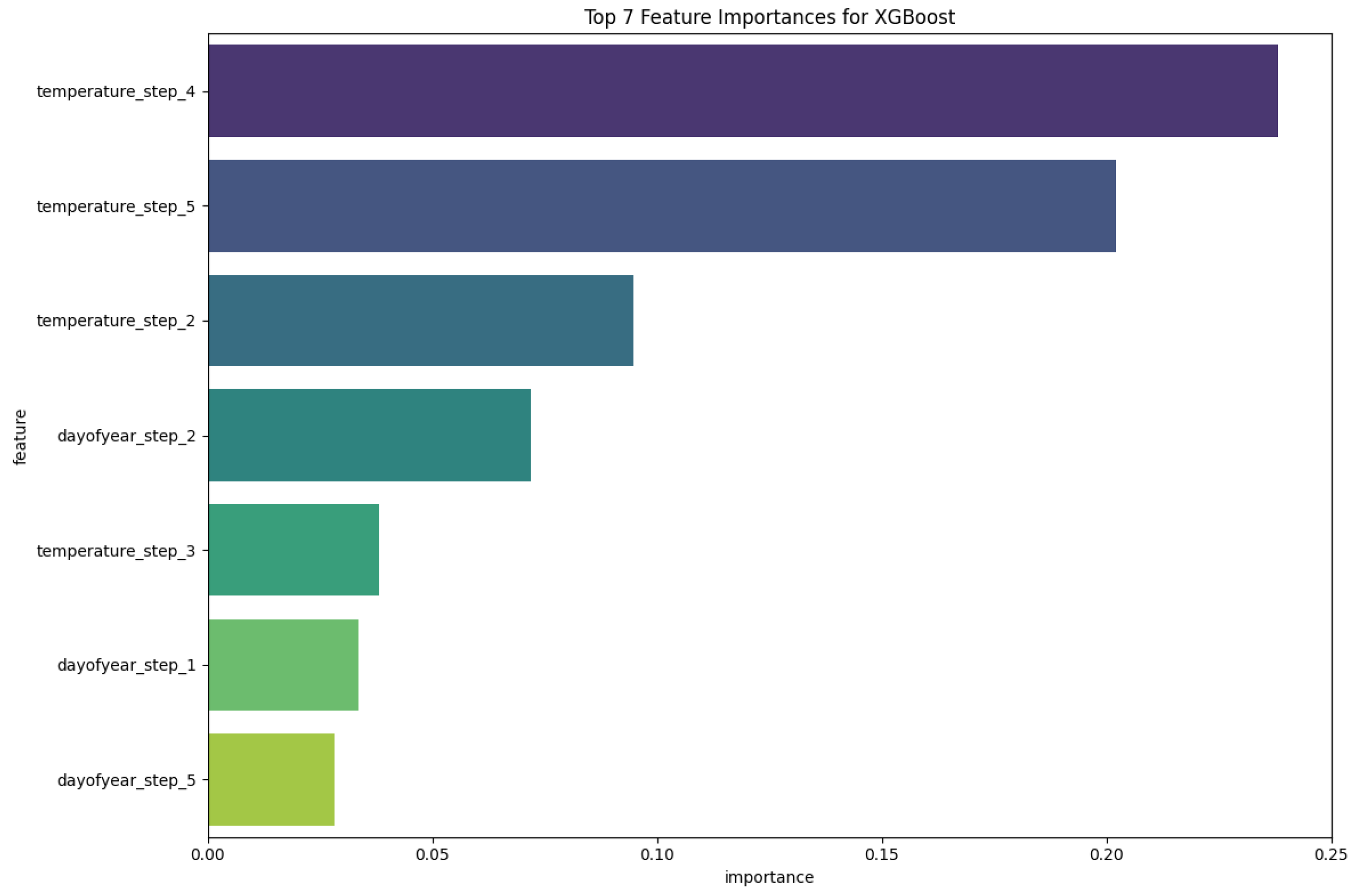
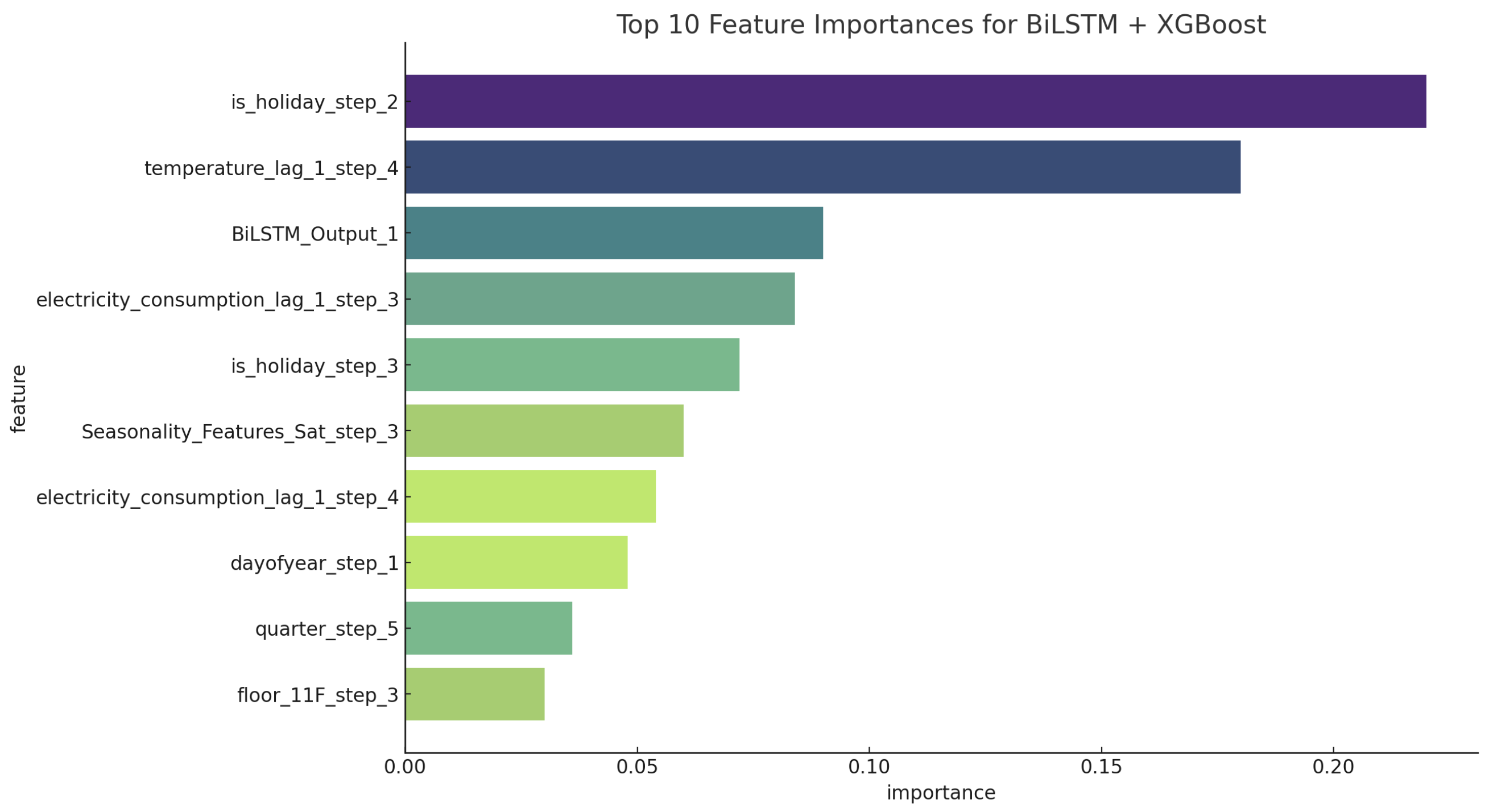
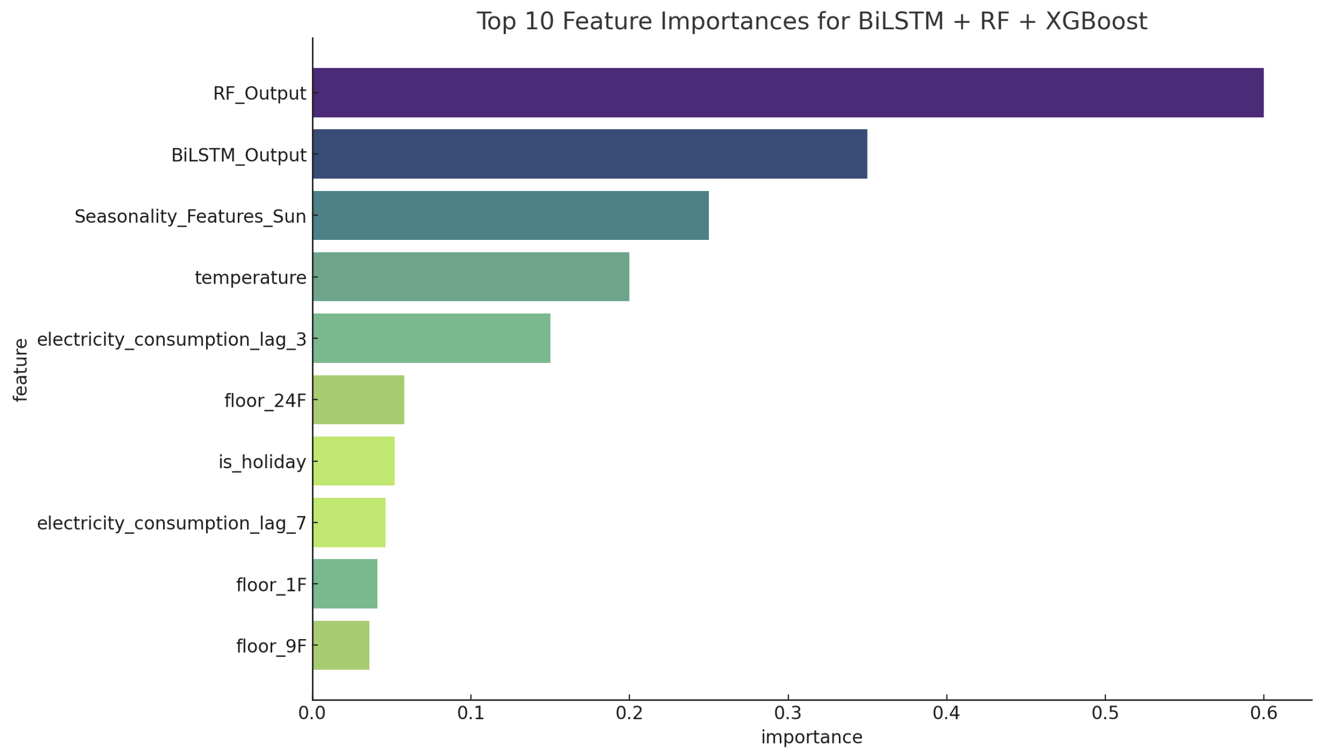
4.4. Feature Importance Analysis

Feature importance analysis is an important tool to help the stakeholders understand which input variables are more influential to the model decision and training performance by measuring each feature’s contribution to the model prediction results. In this study, the SHAP method is mainly used to quantify the contribution of each feature to the model prediction results and to enhance the overall interpretability of the model. SHAP is a game-theory based method that explains the output of a learning model by assigning an importance value (SHAP value) to each feature in a single prediction.

In addition, feature significance analysis can be used as an important basis for the selection of model features in subsequent studies. In the face of datasets with high feature dimensions and complexity, the selection of input features is very important. By distinguishing less influential feature factors, researchers can consider removing these unimportant input features in subsequent improvement work, which not only simplifies the model structure and reduces the risk of overfitting of the model but also enhances the model’s generalization ability and operational efficiency. In addition, feature importance analysis can transform professional prediction tasks into easy-to-explain knowledge content for the outside world, even for non-technical people. Researchers can help others understand what factors are affecting the prediction of electricity consumption in buildings through this visualization of feature importance bar charts, which plays a positive role in the wide dissemination of the model and its application.

The study visualizes feature influence histograms and SHAP swarm plots for the XGBOOST, BILSTM+XGBOOST, and BILSTM+RF+XGBOOST hybrid models, which will be analyzed next. Combining the XGBOOST feature influence histogram in Figure 15 and the SHAP swarm plot of the XGBOOST model in Figure 16, it can be seen that for the single XGBOOST model, the temperature feature is the most dominant feature influence factor, and the SHAP value reflects the fact that the electricity demand is strongly influenced by the temperature of cooling and heating, and an increase in temperature also brings about an increase in the predicted value. The time lag feature highlights the autocorrelation of the electricity consumption time series. These demonstrate the greater dependence of model output on direct temperature and time features when the model operates independently and without stratified features from other models.

As shown in Figure 17 and Figure 18, the BILSTM+XGBOOST model progressively increases the importance weight of holiday features to the model as its learning power increases. The SHAP analysis reveals a shift in feature importance, with the presence of holidays significantly improving the predicted values. The BILSTM model is likewise highly influential on the output of a step in the future, which suggests that the XGBOOST meta-learner relies on the time series representation learned by BILSTM.

In addition, the electric consumption lag feature and the temperature feature also show a high influence. If readers combine this with real life, they will also find that the difference between the electricity demand on holidays and weekdays is very large, which indicates that this study’s exploration of the influence of holiday features is in line with the actual situation. In addition, the output feature BILSTM_Output_1 of the BILSTM model occupies a significant position in this model, which indicates that the BILSTM model effectively extracts valuable feature information from the time series data and then inputs it into the XGBOOST model to help its training and learning, which improves the prediction performance of the hybrid model.

The feature influence histogram of the BILSTM+RF+XGBOOST stacked hybrid model proposed in this study is shown in Figure 19 and the SHAP swarm diagram is shown in Figure 20. The output features ‘RF_Output’ and ‘BILSTM_Output’ of the base model undoubtedly become the most dominant features. In the SHAP plot, we can clearly notice that higher output values from the RF and BILSTM base models (darker purple dots in Figure 20) lead to higher positive SHAP values, which help the model to strongly pull up the final prediction; on the contrary, lower base model output values (lighter yellow dots in Figure 20) lead to negative SHAP values, which pull down the prediction. This clearly demonstrates that in this multi-model stacking architecture, the predictions of the two base models are the input features on which the meta-learner XGBOOST model relies the most. It also demonstrates to the reader that it is feasible to significantly improve the prediction performance by effectively combining the outputs of different base models as input information. The base data features, such as temperature features, electricity consumption lag features, and holiday features, still retain some importance in the meta-learner because this original feature information still plays a complementary role in the prediction process of the stacked model.

In summary, the SHAP feature significance analysis used in this study not only verifies the key roles of temperature, lagged consumption, and holidays in the building electricity prediction task but also presents to the readers the practical basis for the stacked model proposed in this study to significantly improve the prediction performance, which provides a clearer and more convincing reference for the design and energy optimization of future electricity consumption prediction models.

5. Conclusions and Prospect

This study effectively demonstrates to the readers the excellent performance of the hybrid BILSTM-RF-XGBOOST model in building electricity consumption prediction and explores its potential for future applications in energy management and energy optimization. The model uses a Bayesian algorithm to find the optimal hyperparameters to enhance the model performance, while strict K-fold time series cross-validation is used to minimize the risk of overfitting. Experimental results on an independent test set show that this stacked model can effectively combine the time series feature extraction capability with the nonlinear fitting capability of the model to significantly improve the accuracy of electricity consumption prediction in buildings. In this study, the search space and the number of iterations are explicitly defined for the Bayesian so that it plays a key role in the model validation process. With the help of this algorithm, this study not only finds the global optimal solution for the hyperparameters, but also reduces the application cost and time cost of the model calculation. The SHAP feature significance analysis in this study not only provides an in-depth explanation of the model decision-making mechanism but also verifies that the model learning mechanism has plausible physical significance and interpretability, which provides an important guidance for the subsequent optimization of feature engineering. The full paper demonstrates the excellent performance and persuasiveness of the BILSTM-RF-XGBOOST stacked hybrid model proposed in this study in the complex task of power consumption prediction in buildings from various perspectives, which lays the foundation for the expansion and extension of future research directions.

Although the BILSTM-RF-XGBOOST hybrid model proposed in this study has achieved satisfactory results in building power consumption prediction, there is still the most important work waiting to be accomplished for future research. First of all, the study’s current work on feature engineering is still at a relatively simple and rough stage, and in future work, researchers must focus on considering the introduction of Fourier transforms to model periodicity more explicitly, developing more complex sliding window features, or integrating more detailed weather interaction terms with access to relevant data to further improve the model’s interpretability and robustness by introducing more external factors.

Meanwhile, the shortcoming of this study is the lack of comparison with other advanced hybrid models and some new architectures (e.g., the Transformer model), while the experimental phase of some base models might be better improved by introducing an attention mechanism or data augmentation to improve the fit of the base model, thus comparing the performance modification of the hybrid models in a more significant and convincing way. Realizing the fair tuning of many different complex hybrid models for reference and improving the comparability of the base model will be a necessary focus in the future.

And as the core of this study, what Bayesian optimization algorithms need to achieve in future work is to further improve the presentation of this part by supplementing the convergence curves of the core model, exploring the visualization of the surface of the local objective function, and performing hyperparameter sensitivity analyses to improve the clarity and depth of the study.

In summary, while certain achievements have been made, it is important for researchers to bear in mind that addressing and refining the current deficiencies in the future will not only further improve the current model, but will also contribute to the wider field of energy prediction by providing a more robust, interpretable and applicable research solution to support more effective energy management in low carbon buildings.

References

1. Sathishkumar, V.E.; Lee, M.; Lim, J.; Kim, Y.; Shin, C.; Park, J.; Cho, Y. An energy consumption prediction model for smart factory using data mining algorithms. KIPS Trans. Softw. Data Eng. 2020, 9, 153–160. [Google Scholar]
2. Bilgili, M.; Pinar, E. Gross electricity consumption forecasting using LSTM and SARIMA approaches: A case study of Türkiye. Energy 2023, 284, 128575. [Google Scholar] [CrossRef]
3. Ribeiro, A.M.N.C.; do Carmo, P.R.X.; Rodrigues, I.R.; Sadok, D.; Lynn, T.; Endo, P.T. Short-term firm-level energy-consumption forecasting for energy-intensive manufacturing: A comparison of machine learning and deep learning models. Algorithms 2020, 13, 274. [Google Scholar] [CrossRef]
4. Semmelmann, L.; Henni, S.; Weinhardt, C. Load forecasting for energy communities: A novel LSTM-XGBoost hybrid model based on smart meter data. Energy Inform. 2022, 5, 24. [Google Scholar] [CrossRef]
5. Zhang, L.; Shi, J.; Wang, L.; Xu, C. Electricity, heat, and gas load forecasting based on deep multitask learning in industrial-park integrated energy system. Entropy 2020, 22, 1355. [Google Scholar] [CrossRef]
6. Tang, C.; Zhang, Y.; Wu, F.; Tang, Z. An improved cnn-bilstm model for power load prediction in uncertain power systems. Energies 2024, 17, 2312. [Google Scholar] [CrossRef]
7. Peng, B.; Liu, L.; Wang, Y. Monthly electricity consumption forecast of the park based on hybrid forecasting method. In Proceedings of the China International Conference on Electricity Distribution (CICED), Shanghai, China, 7–9 April 2021; IEEE: Piscataway, NJ, USA, 2021; pp. 789–793. [Google Scholar]
8. Son, N.; Shin, Y. Short-and medium-term electricity consumption forecasting using Prophet and GRU. Sustainability 2023, 15, 15860. [Google Scholar] [CrossRef]
9. Essien, A.; Giannetti, C. A deep learning model for smart manufacturing using convolutional LSTM neural network autoencoders. IEEE Trans. Ind. Inform. 2020, 16, 6069–6078. [Google Scholar] [CrossRef]
10. Liu, F.; Liang, C. Short-term power load forecasting based on AC-BiLSTM model. Energy Rep. 2024, 11, 1570–1579. [Google Scholar] [CrossRef]
11. Pooniwala, N.; Sutar, R. Forecasting short-term electric load with a hybrid of arima model and lstm network. In Proceedings of the International Conference on Computer Communication and Informatics (ICCCI), Coimbatore, India, 27–29 January 2021; IEEE: Piscataway, NJ, USA, 2021; pp. 1–6. [Google Scholar]
12. Luo, S.; Wang, B.; Gao, Q.; Wang, Y.; Pang, X. Stacking integration algorithm based on CNN-BiLSTM-Attention with XGBoost for short-term electricity load forecasting. Energy Rep. 2024, 12, 2676–2689. [Google Scholar] [CrossRef]
13. Shi, Z.; Zhou, X.; Zhang, J.; Zhang, A.; Shi, G.; Yang, Q. UAV Trajectory Prediction Based on Flight State Recognition. IEEE Trans. Aerosp. Electron. Syst. 2023, 60, 2629–2641. [Google Scholar]
14. Gustafsson, O.; Villani, M.; Stockhammar, P. Bayesian optimization of hyperparameters from noisy marginal likelihood estimates. J. Appl. Econ. 2023, 38, 577–595. [Google Scholar] [CrossRef]
15. Pierre, A.A.; Akim, S.A.; Semenyo, A.K.; Babiga, B. Peak electrical energy consumption prediction by ARIMA, LSTM, GRU, ARIMA-LSTM and ARIMA-GRU approaches. Energies 2023, 16, 4739. [Google Scholar] [CrossRef]
16. Shi, Z.; Jia, Y.; Shi, G.; Zhang, K.; Ji, L.; Wang, D.; Wu, Y. Design of Motor Skill Recognition and Hierarchical Evaluation System for Table Tennis Players. IEEE Sens. J. 2024, 24, 5303–5315. [Google Scholar] [CrossRef]
17. Shi, Z.; Shi, G.; Zhang, J.; Wang, D.; Xu, T.; Ji, L.; Wu, Y. Design of UAV Flight State Recognition System for Multisensor Data Fusion. IEEE Sens. J. 2024, 24, 21386–21394. [Google Scholar] [CrossRef]
18. Zhang, F.; Yu, Z.; Yuan, S.; Lan, G. Short Term Power Load Forecasting Model Based on XGBoost-BiLSTM. In Proceedings of the 9th International Conference on Power and Renewable Energy (ICPRE), Shanghai, China, 20–22 March 2024; IEEE: Piscataway, NJ, USA, 2024; pp. 1691–1694. [Google Scholar]
19. Chen, Y.; Fu, Z. Multi-step ahead forecasting of the energy consumed by the residential and commercial sectors in the United States based on a hybrid CNN-BiLSTM model. Sustainability 2023, 15, 1895. [Google Scholar] [CrossRef]
20. Bouktif, S.; Fiaz, A.; Ouni, A.; Serhani, M.A. Multi-sequence LSTM-RNN deep learning and metaheuristics for electric load forecasting. Energies 2020, 13, 391. [Google Scholar] [CrossRef]
21. Al-Jamimi, H.A.; BinMakhashen, G.M.; Worku, M.Y.; Hassan, M.A. Advancements in household load forecasting: Deep learning model with hyperparameter optimization. Electronics 2023, 12, 4909. [Google Scholar] [CrossRef]
22. Chang, W.; Chen, X.; He, Z.; Zhou, S. A prediction hybrid framework for air quality integrated with W-BiLSTM (PSO)-GRU and XGBoost methods. Sustainability 2023, 15, 16064. [Google Scholar] [CrossRef]
23. Yang, F.; Yan, K.; Jin, N.; Du, Y. Multiple households energy consumption forecasting using consistent modeling with privacy preservation. Adv. Eng. Inform. 2023, 55, 101846. [Google Scholar] [CrossRef]
24. Liu, D.; Sun, K. Random forest solar power forecast based on classification optimization. Energy 2019, 187, 115940. [Google Scholar] [CrossRef]
25. Zhang, T.; Zhang, X.; Liu, Y.; Chow, Y.H.; Iu, H.H.-C.; Fernando, T. Long-term energy and peak power demand forecasting based on sequential-XGBoost. IEEE Trans. Power Syst. 2023, 39, 3088–3104. [Google Scholar] [CrossRef]
26. Hajj-Hassan, M.; Awada, M.; Khoury, H.; Abou Saleh, Z. A behavioral-based machine learning approach for predicting building energy consumption. In Proceedings of the Construction Research Congress 2020, Tempe, AZ, USA, 8–10 March 2020; American Society of Civil Engineers (ASCE): Reston, VA, USA, 2020; pp. 1029–1037. [Google Scholar]
27. Sun, D.; Xu, J.; Wen, H.; Wang, D. Assessment of landslide susceptibility mapping based on Bayesian hyperparameter optimization: A comparison between logistic regression and random forest. Eng. Geol. 2021, 281, 105972. [Google Scholar] [CrossRef]
28. Joy, T.T.; Rana, S.; Gupta, S.; Venkatesh, S. Batch Bayesian optimization using multi-scale search. Knowl.-Based Syst. 2020, 187, 104818. [Google Scholar] [CrossRef]
Figure 1. The unit structure of LSTM.
Electronics 14 02287 g001
Figure 2. The unit structure of BILSTM.
Electronics 14 02287 g002
Figure 3. Structure diagram of RF algorithm.
Electronics 14 02287 g003
Figure 4. Structure diagram of XGBOOST algorithm.
Electronics 14 02287 g004
Figure 5. The implementation process of the hybrid model.
Electronics 14 02287 g005
Figure 6. Total daily electricity consumption of the building.
Electronics 14 02287 g006
Figure 7. RNN prediction vs. true values Bayes (CV).
Electronics 14 02287 g007
Figure 8. LSTM prediction vs. true values Bayes (CV).
Electronics 14 02287 g008
Figure 9. BILSTM prediction vs. true values Bayes (CV).
Electronics 14 02287 g009
Figure 10. XGBOOST prediction vs. true values Bayes (CV).
Electronics 14 02287 g010
Figure 11. BILSTM-XGBOOST prediction vs. true values Bayes (CV).
Electronics 14 02287 g011
Figure 12. BILSTM-RF-XGBOOST prediction vs. true values Bayes (CV).
Electronics 14 02287 g012
Figure 13. All model comparison: trues vs. predictions.
Electronics 14 02287 g013
Figure 14. Line graph of hybrid model prediction results (test set).
Electronics 14 02287 g014
Figure 15. Feature importance for XGBOOST.
Electronics 14 02287 g015
Figure 16. SHAP beeswarm plot for XGBOOST.
Electronics 14 02287 g016
Figure 17. Feature importance for BILSTM-XGBOOST.
Electronics 14 02287 g017
Figure 18. SHAP beeswarm plot for BiLSTM + XGBoost.
Electronics 14 02287 g018
Figure 19. Feature importance for BILSTM+RF+XGBOOST.
Electronics 14 02287 g019
Figure 20. SHAP beeswarm plot for BiLSTM + RF + XGBoost.
Electronics 14 02287 g020