Abstract
To address the conflicting demands of the energy crisis, environmental pollution, and economic growth, the electric vehicle (EV) industry has expanded rapidly, facilitating the widespread adoption of power batteries. This paper investigates the use of chaos theory and machine learning for predicting the remaining useful life (RUL) of lithium-ion batteries. Firstly, the mutual information method determines the time delay of the monitoring sequence, while the improved false nearest neighbor method (Cao algorithm) establishes the embedding dimension, yielding the phase space reconstruction parameters. Secondly, the maximum Lyapunov exponent identifies the chaotic properties of the capacity decay time series, and a prediction dataset is constructed based on phase space reconstruction theory. Finally, leveraging the chaotic time-series features, a support vector machine (SVM) model is developed for lithium-ion battery RUL prediction. The algorithm is subsequently validated through simulation using the NASA battery dataset. The results demonstrate that the proposed method achieves high predictive accuracy and stability, providing reliable RUL estimates for the battery management system (BMS).
1. Introduction
With the growing global demand for clean energy and increased environmental awareness, lithium-ion batteries—as efficient and recyclable energy storage devices—have been widely employed across various sectors, including electric vehicles, portable electronics, and renewable energy storage systems [1]. However, during actual operation, lithium-ion batteries inevitably undergo complex aging mechanisms, leading to performance degradation—such as capacity fade and elevated internal resistance—which adversely affects their RUL [2]. Accurate RUL prediction for lithium-ion batteries is essential for optimizing the BMS, ensuring safe equipment operation, reducing maintenance costs, and enhancing resource utilization efficiency.
At present, the methods for predicting the RUL of lithium-ion batteries primarily comprise model-based, fusion algorithm-based, and data-driven approaches. Model-based methods typically rely on electrochemical models and equivalent circuit models. Gao et al. [3] reported that, with rapid technological advancements, lithium-ion batteries have become the preferred power source for portable applications owing to their compact size, light weight, and diverse form factors, meeting the endurance requirements of modern electronic devices. Wu et al. [4] conducted a comparative analysis to clarify the key parameters, advantages, limitations, and technical bottlenecks of various energy storage technologies. Based on these findings, they assessed the application prospects of these technologies and provided guidance for selecting suitable energy storage solutions in industrial contexts. Li et al. [5] reviewed the principal technical pathways for lithium battery recycling domestically and internationally, with a focus on novel cascade utilization models for power lithium-ion batteries. They further examined the primary challenges facing domestic lithium-ion battery recycling and explored feasible future recycling strategies. J Permana et al. [6] employed coulomb counting to measure the nominal capacity of individual lithium-ion cells under constant current discharge and charging, subsequently extracting equivalent circuit model (ECM) parameters; they noted that estimation accuracy was influenced by current measurement precision and integration errors. Gao et al. [7] enhanced the traditional ampere-hour integration method by accounting for charge–discharge efficiency, temperature, and cycle count to improve state-of-charge (SOC) estimation accuracy. They employed the open-circuit voltage method to estimate the initial SOC and applied the load–voltage method at the end of constant current discharge to correct cumulative SOC estimation errors in real time.
Wang et al. [8] employed an ECM approach. During charging and discharging, the internal chemical reactions—driven by lithium-ion migration between electrodes—exhibit time-varying nonlinear behavior. Consequently, directly deriving accurate model parameters via theoretical analysis is highly challenging. Kong et al. [9] utilized electrochemical impedance spectroscopy to measure battery parameters; however, this technique demands high-precision instrumentation, involves complex procedures, and yields parameters that are variable and difficult to ascertain. Cui et al. [10] incorporated a double-layer electrochemical (DEL) model to account for its effect on electrolyte potential. This model entails numerous partial differential equations and intricate parameters, resulting in high computational cost.
Zhang et al. [11] applied deep learning techniques to estimate SOC. Despite strong data fitting capabilities, deep learning model accuracy is sensitive to data quality and model complexity. Data noise or model overcomplexity leading to overfitting further degrades estimation accuracy. Generalization limitations and limited model interpretability may further constrain performance. Liu [12] proposed an adaptive hybrid unscented Kalman filter (AHUKF) for SOC estimation; however, it did not address noise interference and outlier robustness. Liu et al. [13] implemented an extended particle filter for SOC estimation. However, increased particle counts substantially raise the computational load, and particle degeneracy remains a challenge. Gao et al. [14] developed a fourth-order chaotic system nonlinear combination model, demonstrating improved dynamic estimation accuracy and generalization. Ding et al. [15] proposed a multistep, cell-level data-driven method for accurate thermal runaway prediction. They formulated this as an imbalanced classification problem and introduced a meta-thermal runaway prediction neural network (Meta-TRFNN). They additionally employed a meta-learning framework to mitigate data scarcity.
Zang et al. [16] combined principal component analysis, variational mode decomposition, and long short-term memory (LSTM) networks to predict battery remaining life, enhancing accuracy and resolving issues with health indicator extraction and VMD parameter selection. Lin et al. [17] developed an attention-based gated recurrent unit (Attention-GRU) model for RUL prediction. Xia et al. [18] introduced an RUL prediction method for energy storage lithium-ion batteries, addressing safety concerns arising from battery aging under peak load and frequency regulation conditions. Cai et al. [19] constructed continuous health indicators and combined a generalized regression neural network with an enhanced extreme learning machine (ELM) for multistep RUL prediction. Leo et al. [20] proposed a hybrid model for simultaneous state-of-health (SOH) and RUL prediction: their approach decomposes the capacity signal via improved complementary ensemble empirical mode decomposition with adaptive noise (ICEEMDAN), then applies support vector regression (SVR) to high-frequency components and LSTM to low-frequency components. Wu et al. [21] introduced a progressive prediction framework to enhance RUL accuracy for lithium-ion batteries. Lu et al. [22] proposed a two-stage framework to develop a lithium-ion battery SOH assessment model considering the migration of DM knowledge. The model can effectively preserve the temporal dynamic characteristics of the battery degradation process. Combining data mining (DM) and other related conditions, a CTSGAN-based SOH estimation model was constructed and demonstrated good estimation performance.
This paper presents a hybrid approach integrating chaos theory with a support vector machine (SVM) model to accurately estimate battery RUL. Firstly, the mutual information method determines the time delay of the monitoring sequence, while the improved false nearest neighbor (Cao) algorithm identifies the embedding dimension, yielding phase space reconstruction parameters. Next, the maximum Lyapunov exponent quantifies the chaotic properties of the capacity decay time series, and a prediction dataset is constructed based on phase space reconstruction theory. Subsequently, exploiting chaotic time-series features, an SVM model is trained for lithium-ion battery RUL prediction. The model is then validated through simulation using the NASA battery dataset. The results indicate that the proposed method achieves high predictive accuracy and stability, providing reliable RUL estimates for a BMS.
2. Theoretical Model
2.1. Chaotic Time Series
Chaos theory is a branch of nonlinear system theory. Its core principle is to reconstruct the phase space through time-series embedding, which provides a new dimension for revealing system dynamics, revealing potential order, and predicting future system evolution. Since the capacity decay sequence is not pure random noise, but low-dimensional chaotic behavior, it is difficult for traditional statistical fitting models to capture its internal structure. For chaotic time series, delayed coordinate reconstruction can be used to make more accurate predictions of the RUL of the battery. In this process, the fidelity of the phase space reconstruction is crucial to the accuracy of the system trajectory prediction. Therefore, it is crucial to choose suitable and efficient reconstruction technology. Common reconstruction methods include the derivative method and the coordinate delay method. Compared with the derivative method, the coordinate delay method only requires a one-dimensional time series, which reduces the computational complexity and can obtain a better attractor reconstruction effect. Therefore, this study uses the coordinate delay method to reconstruct the phase space of the time series.
For the time series , the coordinate delay method uses the time delay to construct the dimensional phase space vector:
, is the delay time.
Thus, an dimensional phase space comprising phase points is reconstructed. Here, represents the embedding dimension, and denotes the delay time. The phase points defined by Equation (1) constitute trajectories in the dimensional phase space, and their spatial relationships characterize the system’s chaotic attractor. Hence, the embedding dimension and delay time are critical for reconstructing high-fidelity chaotic attractors. Therefore, the primary task in phase space reconstruction is to determine appropriate values for the embedding dimension and delay time.
2.2. Determine the Delay Time Using the Mutual Information Method
Suppose that the time series , are independent of each other. The information entropy function of the time series can be expressed as follows:
represents the probability of occurrence of the sequence element. Similarly, the information entropy function of time series Y can also be expressed in the form of Equation (3). Then, the joint entropy of the time series can be expressed as follows:
represents the probability of and appearing at the same time. Thus, the mutual information function of the two can be obtained
Generally, the time delay corresponding to the first minimum value of the mutual information function is taken as the time delay .
2.3. CAO Method to Determine the Embedding Dimension
Cao’s method is an enhanced version of the pseudo-nearest neighbor technique. This technique requires only the delay time to compute the embedding dimension , thereby eliminating user-dependent bias. Moreover, it demands less time-series data, making it particularly suitable for real-world applications. The procedure can be summarized as follows:
Among them, and are the -th phase point vector and its nearest neighbor in the dimensional space. Define the mean of all to be as follows:
At the same time, the change in the mean from dimension to dimension is defined as follows:
The statistic characterizes the time series and identifies its optimal embedding dimension. If the series is purely random, increases monotonically with the embedding dimension ; in contrast, for deterministic series, converges and stabilizes as increases. Thus, the value at which first stabilizes is deemed the optimal embedding dimension. Because convergence can be difficult to discern in practice, a quantitative criterion is introduced in Equation (4):
For random sequences, is always 1; for deterministic sequences, due to the dependence of the correlation between data on the embedding dimension , there must be a value that does not equal 1 as the embedding dimension increases.
2.4. Determination of Chaotic Characteristics of Time Series
This paper employs the Lyapunov exponent method to assess chaos in time series. The Lyapunov exponent quantifies the asymptotic behavior of trajectories in a nonlinear system, representing the average divergence and convergence rates of neighboring orbits in phase space. The sign of the Lyapunov exponent—positive or negative—indicates the presence or absence of chaotic behavior in the system. Below, we outline the algorithm for computing the Lyapunov exponent. Consider the first-order linear differential equation:
The analytical solution of Equation (1) is
Consider two infinitesimally close trajectories at the initial time: if , their separation grows exponentially and the trajectories diverge; if , their separation decays exponentially and the trajectories converge; if , their separation remains constant. For a nonlinear system, linearization around a reference state provides a local linear approximation. Mathematically, a continuous non-autonomous system is described by the differential equation:
There are convergence and divergence directions at the initial value , is a nonlinear function, which is
Its linearization matrix is the Jacobian matrix
Let the neighborhood of be
In Equation (3), is the deviation. Substituting Equation (3) into Equation (2), the equation of the deviation is obtained after linearization:
Solving Equation (4), we obtain
In Equation (5), is the initial deviation and is the eigenvalue of matrix . The Lyapunov exponent is as follows:
In Equation (6), represents the average change in the deviation over a long period of time, that is, the Lyapunov index. There are components in the Jacobian matrix , and the number of corresponding Lyapunov exponents is , which are arranged , according to their size, into the Lyapunov index spectrum:
If > 0 ( = 1, 2 … n), it means that the orbit around is moving away from along the direction , the nonlinear system is locally unstable, the adjacent orbits are separated exponentially, the system has chaotic behavior, and when there is a Lyapunov index greater than zero in the nonlinear system, the system will experience chaos; when there are two or more Lyapunov indexes greater than zero in the system, the system will experience hyper chaos.
If < 0 ( = 1, 2…n), it means that the orbit around is close to along the direction , the nonlinear system is locally stable, corresponding to the periodic trajectory motion, and the system has no chaotic behavior.
If = 0 ( = 1, 2…n), it means that the orbit around moves along the tangent of , the initial error does not change, and the system boundary is stable.
In the prediction of battery capacity decay, the maximum Lyapunov exponent is not only the core indicator of the feasibility of quantitative prediction, but also the key parameter for guiding model selection, window design, uncertainty assessment, and dynamic early warning. By combining the maximum Lyapunov exponent with the phase space prediction method, the accuracy and reliability of the remaining life estimation can be significantly improved. When > 0 ( = 1, 2…n), the attenuation process is exponentially sensitive to the initial disturbance, and the prediction error grows exponentially with the number of cycles. Therefore, high accuracy can only be obtained within a limited short-term window. At this time, it is appropriate to adopt “local-short-term” prediction methods such as local linear mapping or a short-term memory neural network; when < 0 ( = 1, 2…n), the orbit shows a convergence trend, the noise effect is attenuated, the attenuation curve is smooth and stable, and extrapolation of longer periods is allowed. It is suitable to use global fitting models such as polynomial regression or ARIMA; and when = 0 ( = 1, 2…n), the system is in a boundary stable state, with both periodic oscillation and weak divergence characteristics. The periodic component should be stripped off in combination with frequency domain analysis, and local and global models should be mixed on different time scales to obtain the best prediction performance and operation and maintenance efficiency.
2.5. SVM Model
Support vector machine (SVM) is a supervised learning algorithm utilized for both classification and regression tasks. The core principle involves transforming the original problem into a linearly separable one by constructing an optimal separating hyperplane. The separation hyperplane can be mathematically defined as follows:
is the normal vector and is the displacement term.
In order to maximize the hyperplane distance, the following formula is solved:
The purpose of regression prediction based on SVM is to make and as close as possible. The core idea of support vector regression (SVR) is to assume that the loss is calculated only when the absolute difference between and is greater than . So, the SVR problem can be transformed into
is the regularization constant; is the insensitive loss function. By introducing the slack variable points, the above formula can be written as
To find its minimum value, by introducing Lagrange multipliers , , , , we can obtain the SVR dual problem:
The above process must meet the KKT conditions, which require the following:
It can be seen that the solution of SVR is expressed as
The regression estimation function can be expressed as
where is the kernel function, and this paper chooses the linear kernel function. The penalty coefficient of the SVM is set to 1, the learning rate is set to 0.01, and the maximum number of iterations is 1000.
3. Experiment and Evaluation
3.1. Experimental Data
This study utilizes the NASA Prognostics Center of Excellence (PCOE) battery datasets B0005–B0007 and B0018. These datasets employ 18,650 lithium-ion cells rated at 2 Ah capacity and 4.2 V voltage. A battery aging acceleration test bench was employed to conduct accelerated life testing. At room temperature, cells were initially charged at a constant current of 1.5 A. Once the voltage reached 4.2 V, constant voltage charging continued until the current declined to 20 mA. Subsequently, cells were discharged at a constant current of 2 A until the voltage reached the specified cut-off level. This charge–discharge cycle was repeated until the cells met the end-of-life criterion.
3.2. Model Evaluation Indicators
This study employs the root mean square error (RMSE) and the coefficient of determination (R2 score)—two metrics for quantifying prediction error—to assess the accuracy of the machine learning model. Their mathematical definitions are as follows:
where is the number of samples, is the true value, is the predicted value, and is the average of the true values.
3.3. Experimental Procedure
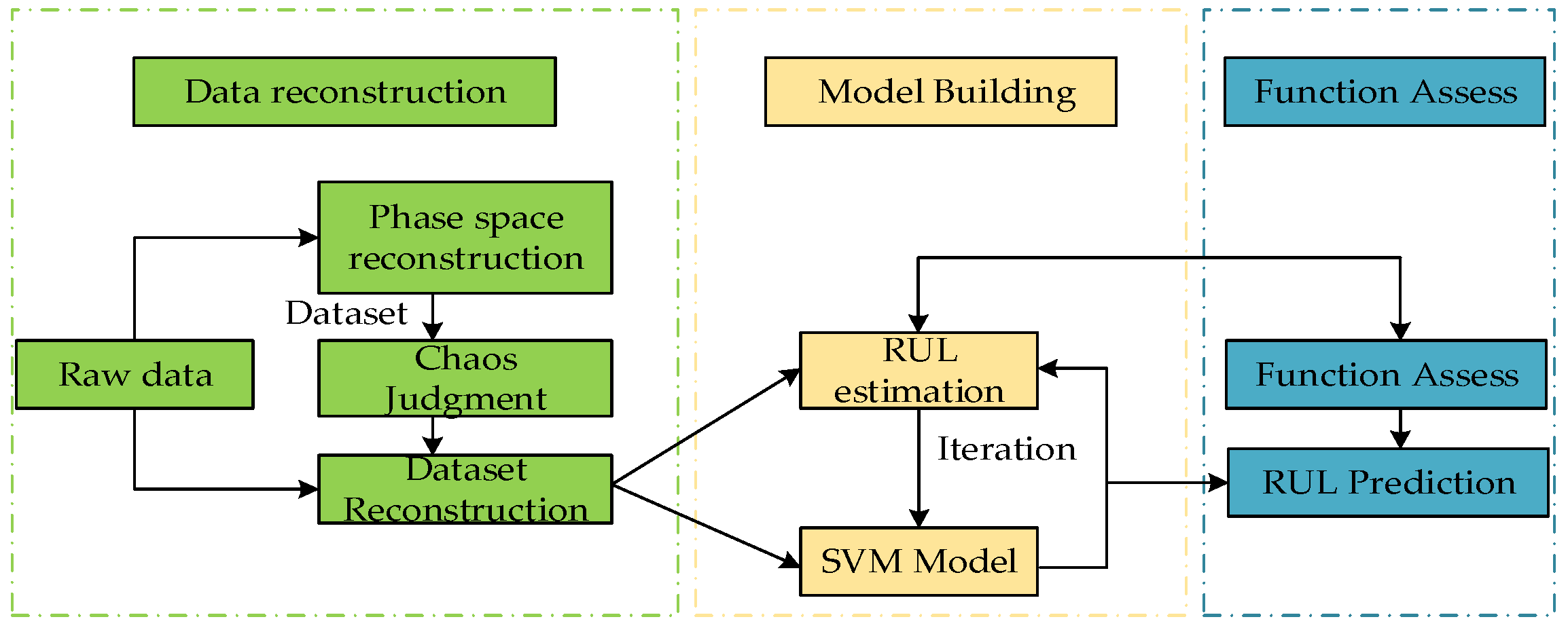
Firstly, the mutual information method determines the delay time, and the Cao algorithm identifies the embedding dimension, enabling phase space reconstruction of the original dataset. Next, the Lyapunov exponent is computed to verify the presence of chaos in the reconstructed system. Finally, the reconstructed data are used to train and validate the predictive model. The specific process is shown in Figure 1.
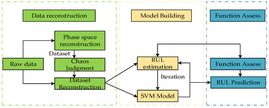
Figure 1.
Experimental flow chart.
4. Simulation Results and Analysis
Because accurate RUL prediction for lithium-ion batteries requires comprehensive, long-term SOH datasets, this study selects NASA batteries B0005, B0006, B0007, and B0018—each with over 100 cycles of SOH records—as the research subjects.
4.1. Phase Space Reconstruction
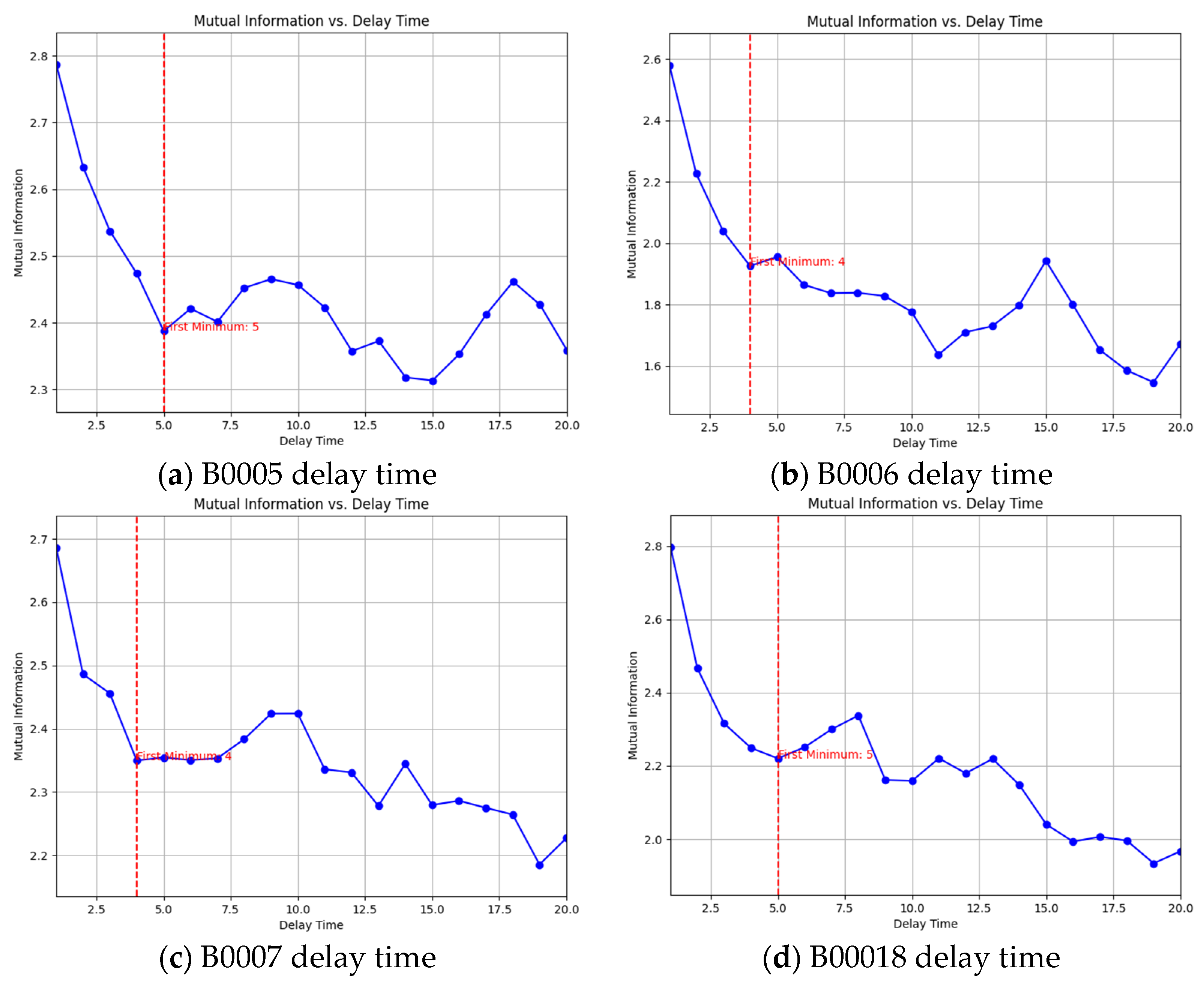
Phase space reconstruction is a prerequisite for analyzing lithium-ion battery capacity decay time series. This study employs the mutual information method to determine the time delay τ; the resulting τ values for four battery types are displayed in Figure 2a–d.
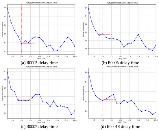
Figure 2.
Mutual information method to calculate delay time τ. The blue line in the figure is the delay time, and the red line is the delay time point when the minimum value is reached for the first time, which is used as the input of the CAO method.
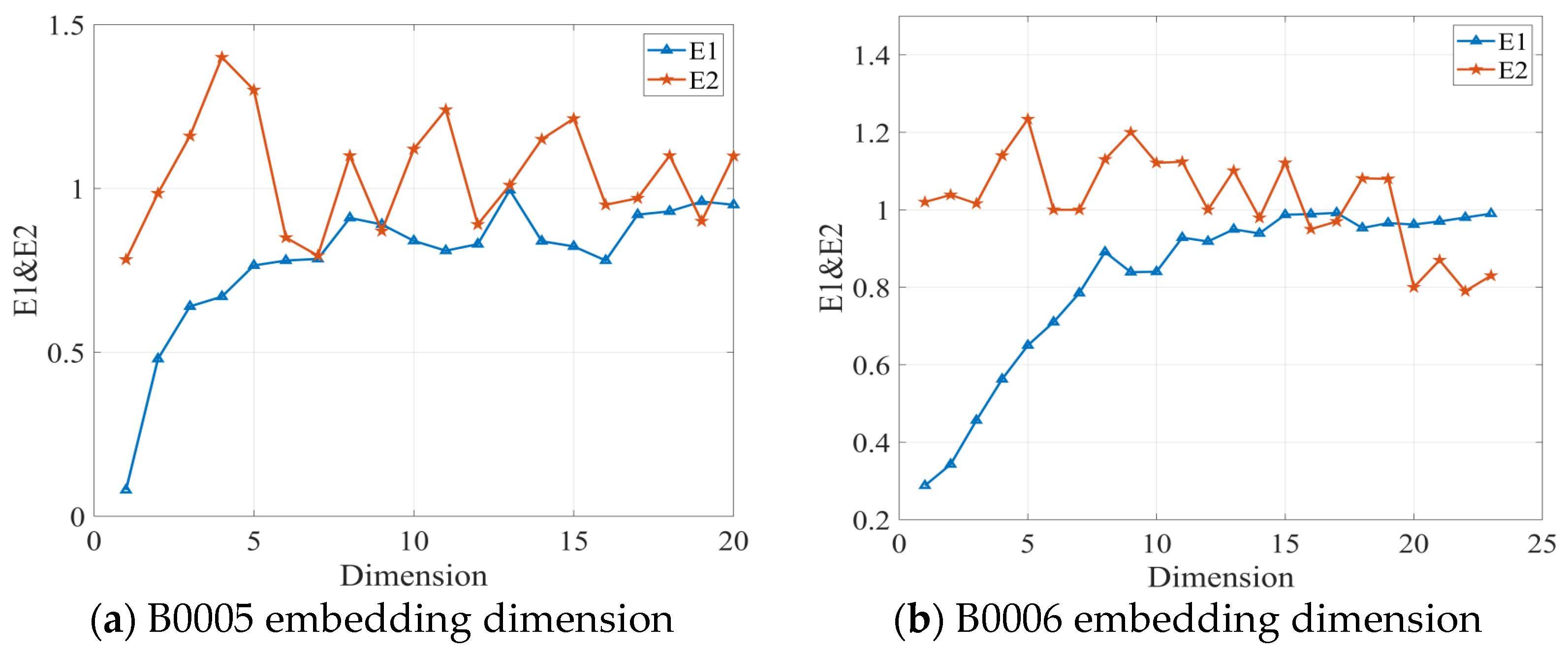
According to the definition of the mutual information method, the time delay corresponding to the first minimum value of the mutual information function I(X,Y) is taken as the time delay. Combined with the calculation results of Figure 2, it can be obtained that the time delay of the phase space reconstruction of the capacity decay time series of battery B0005 is 5, the time delay of the phase space reconstruction of the capacity decay time series of battery B0006 is 4, the time delay of the phase space reconstruction of the capacity decay time series of battery B0007 is 4, and the time delay of the phase space reconstruction of the capacity decay time series of battery B0018 is 5. After obtaining the delay time, the CAO method can be used to find the optimal embedding dimension. Figure 3 shows the relationship diagram of the optimal embedding dimension–E1&E2 for four different types of batteries using the CAO method.
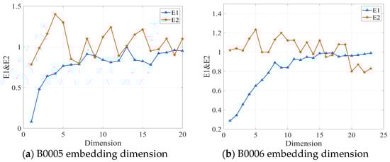
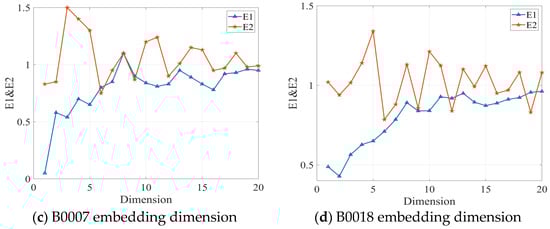
Figure 3.
CAO method optimal embedding dimension–E1&E2 relationship diagram.
According to Cao’s method, the optimal embedding dimension is the smallest for which saturates and is not always 1, since does not always equal unity. The selected optimal embedding dimensions for each dataset are summarized in Table 1.

Table 1.
Delay time, embedding dimension, and Lyapunov exponent of different batteries.
4.2. SVM Prediction Results
SOH represents the remaining service life of the battery. It is a key variable that characterizes the gradual aging of the battery after multiple cycles. Accurate SOH estimation can determine the RUL of the battery and ensure the length of time the battery can complete the corresponding work.
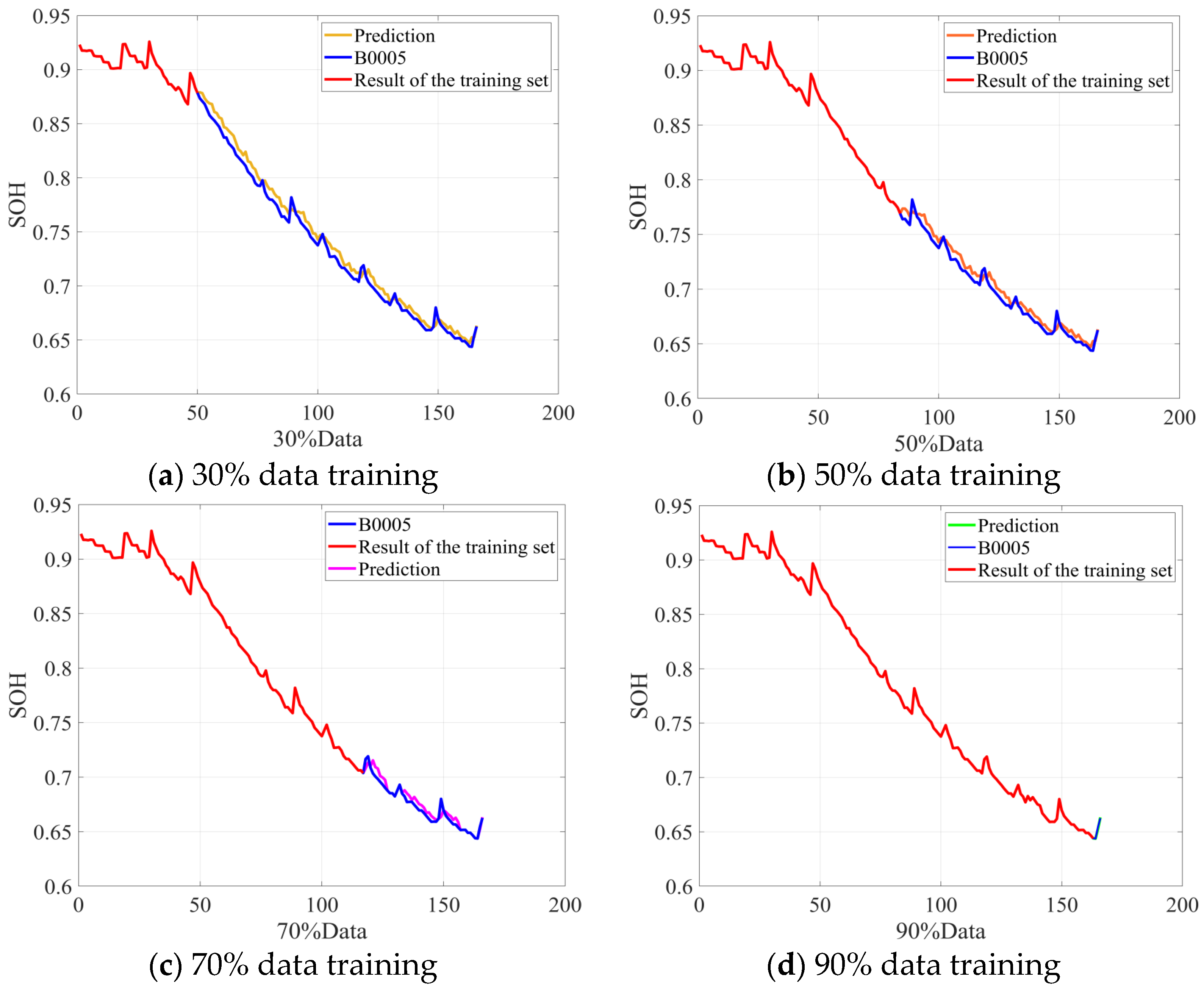
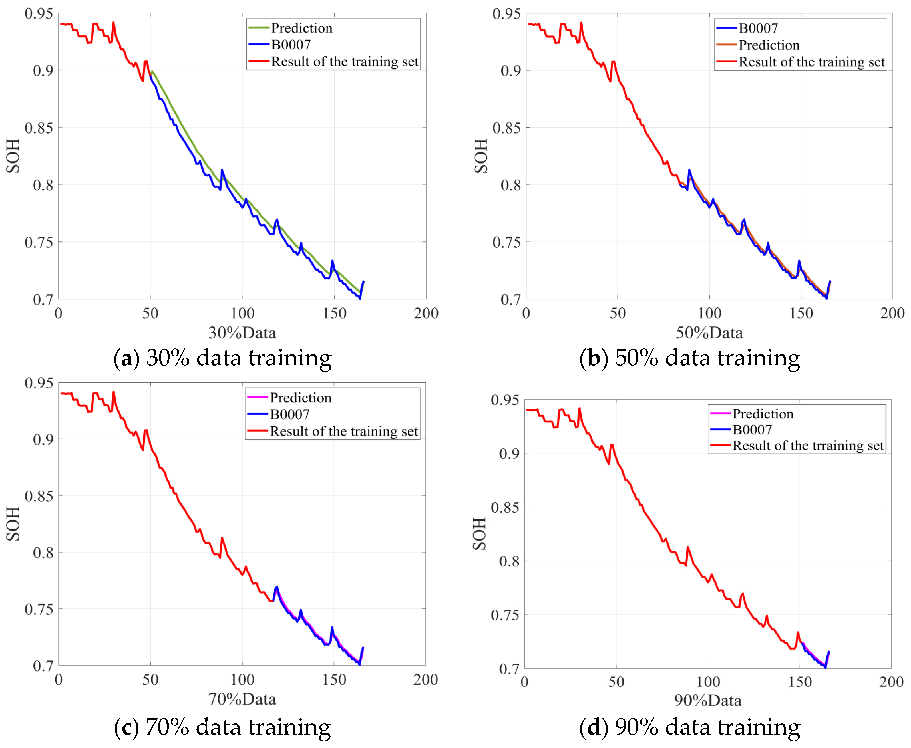
Because chaotic systems are inherently unpredictable over long horizons, using only a subset of data for training yields limited RUL prediction accuracy for lithium-ion batteries. Thus, RUL prediction experiments were conducted with the SVM model on NASA datasets B0005, B0006, and B0007. For each battery, the first 40%, 60%, 80%, and 90% of cycle data served as training sets, while the remaining data comprised test sets for RUL prediction. To assess stability, data from B0005, B0006, and B0007, along with the initial 15% of B0018 data, were combined to train the SVM model, which then predicted the RUL of battery B0018.
Figure 4 illustrates the simulation results for battery B0005. Although the time-series analysis and prediction lack explicit failure characteristic parameters, the model still captures the overall capacity aging trend. As the training data volume increases, the model’s predictive performance steadily improves. Figure 4 also shows that the RUL prediction error decreases progressively as the training dataset expands.
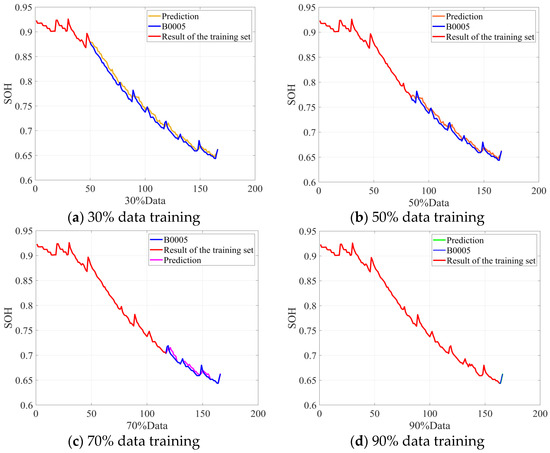
Figure 4.
B0005 battery RUL prediction results.
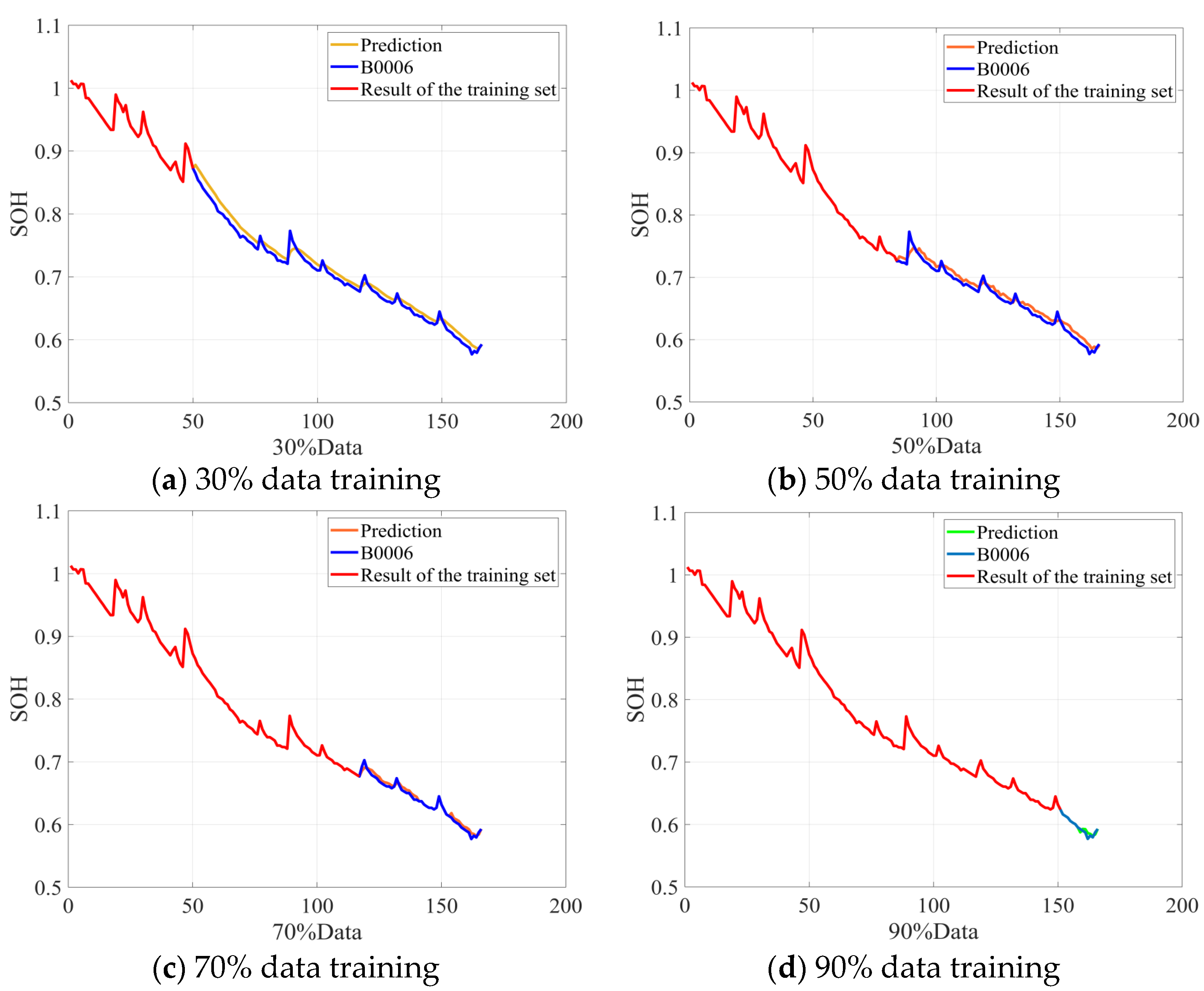
Following the procedure described above, the algorithm was validated on NASA batteries B0006 and B0007. The simulation results for RUL prediction are presented in Figure 5 and Figure 6. These results align closely with those observed for battery B0005. Specifically, as the volume of training data increases, model performance steadily improves. However, the RUL estimates exhibit a positive bias at advanced life stages. This bias arises because, in later cycles, accelerated material degradation intensifies battery nonlinearity, causing the model—trained on current data characteristics—to overestimate the remaining life. Nevertheless, the RUL predictions for batteries B0006 and B0007 remain accurate, further substantiating the proposed algorithm’s efficacy.
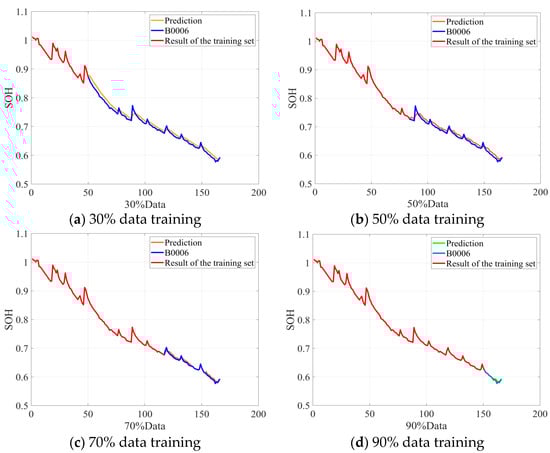
Figure 5.
B0006 battery RUL prediction results.

Figure 6.
B0007 battery RUL prediction results.
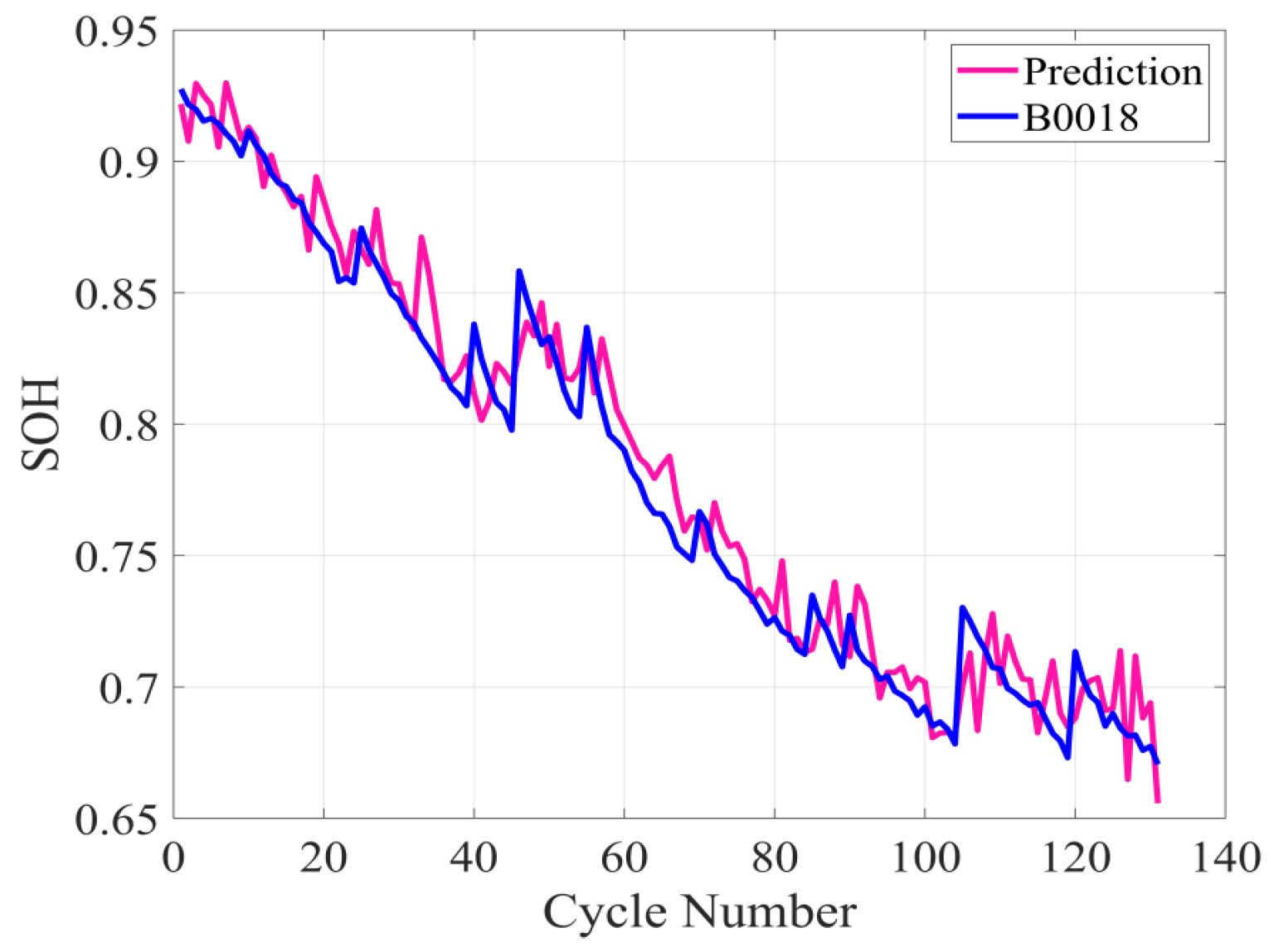
To further validate the proposed method’s predictive capability, the initial 15% of B0018 cycle data were combined with the reconstructed phase space datasets from batteries B0005, B0006, and B0007 to forecast B0018’s RUL. Figure 7 presents the resulting RUL predictions for battery B0018.

Figure 7.
B0018 battery RUL prediction results.
The model achieved a coefficient of determination (R2) of 0.89 and a root mean square error (RMSE) of 0.58%. These performance metrics demonstrate the model’s robust predictive capability. Furthermore, the curve’s peak consistently shifts to the right, corroborating our previous inference. This shift reflects aggravated internal material degradation, which amplifies the battery’s nonlinear dynamics and the long-term unpredictability inherent to chaotic systems.
5. Conclusions
This study presents a chaotic time-series-based method for predicting the RUL of lithium-ion batteries. Firstly, the phase space reconstruction parameters—time delay (τ) and embedding dimension (m)—are determined via the mutual information method and Cao algorithm, and system chaos is confirmed by computing the maximum Lyapunov exponent. Subsequently, an SVM model is developed for RUL prediction. Simulation on NASA datasets B0005, B0006, B0007, and B0018 demonstrates that the prediction accuracy improves progressively with larger training sets, and that the model exhibits robust stability and generalization. Moreover, the proposed approach effectively captures the nonlinear dynamics of capacity decay, delivers reliable RUL estimates for a BMS, and holds significant practical value. Future work will focus on optimizing the model parameters and identifying additional features to enhance prediction accuracy.
Author Contributions
Conceptualization, T.Z.; methodology, T.Z.; software, T.Z.; validation, T.Z. and H.S.; formal analysis, T.Z.; investigation, T.Z.; resources, T.Z.; data curation, T.Z.; writing—original draft preparation, T.Z.; writing—review and editing, T.Z.; visualization, T.Z.; supervision, H.S.; project administration, T.Z. All authors have read and agreed to the published version of the manuscript.
Funding
This research received no external funding.
Data Availability Statement
The data used in this article comes from NASA Ames Research Center, which can be obtained on its official website.
Conflicts of Interest
The authors declare no conflicts of interest.
References
- Sun, Y.; Gong, Y.; Dong, L.; Wang, X.; Yan, Y.; Tang, X.; Dang, Y. A review of state estimation of battery energy storage systems. J. Cent. South Univ. Sci. Technol. 2024, 55, 2320–2333. [Google Scholar]
- Yang, T.; Shen, J.; Guan, Y.; Jiang, T.; Liu, Q. Research on battery life prediction based on early aging and transfer learning. Hunan Electr. Power 2025, 45, 1–7. [Google Scholar]
- Gao, X.; Zhang, L.; Zhao, Y.; Liang, X. A preliminary study on the development of mobile power lithium battery technology. New Mater. Ind. 2021, 3, 60–64. [Google Scholar]
- Wu, H.; Wang, J.; Gong, Y.; Yang, H.; Zhang, M.; Huang, Z. Analysis on the development status and application prospects of energy storage technology. J. Electr. Power 2021, 36, 434–443. [Google Scholar]
- Li, Z.; Zhang, M.; Sun, Z.; Meng, X.; Zhao, P. Current status of waste lithium-ion battery recycling. Chem. Def. Res. 2024, 3, 22–30. [Google Scholar]
- Permana, J.; Manvi, T.; Prajitno, P. State of Charge Estimation of Lithium Ion Battery Using Coulomb Counting Method Based on Raspberry Pi. In Proceedings of the 2024 4th International Conference of Science and Information Technology in Smart Administration (ICSINTESA), Balikpapan, Indonesia, 12–13 July 2024; pp. 582–586. [Google Scholar]
- Gao, J.; Hu, H.; Yao, S. SOC estimation of lithium-ion battery pack based on improved ampere-hour integration method. J. Hubei Automot. Ind. Univ. 2022, 36, 56–60. [Google Scholar]
- Wang, Y.; Sun, G.; Tian, Y. Estimation of the remaining power of aviation emergency batteries using different models and analysis of estimation accuracy. Power Supply Technol. 2024, 48, 2426–2433. [Google Scholar]
- Kong, L.; Fang, S.; Niu, T.; Chen, G.; Yang, L.; Liao, R. Fast State of Charge Estimation for Lithium-ion Battery Based on Electrochemical Impedance Spectroscopy Frequency Feature Extraction. In IEEE Transactions on Industry Applications; IEEE: Piscataway, NJ, USA, 2024; Volume 60, pp. 1369–1379. [Google Scholar]
- Cui, X.; Lu, X. Order reduction electrochemical mechanism model of lithium-ion battery based on variable parameters. Electrochim. Acta 2023, 446, 142107. [Google Scholar] [CrossRef]
- Zhang, L.; Wu, C.; Huang, X.; Li, Y. Full life cycle state of charge estimation of lithium batteries using deep learning. J. Xi'an Jiaotong Univ. 2024, 58, 36–43. [Google Scholar]
- Liu, S.; Cui, N.; Zhang, C. Lithium-ion battery health status estimation based on AUKF. Power Electron. Technol. 2017, 51, 122–124. [Google Scholar]
- Liu, Y.; Lei, W.; Liu, Q.; Gao, Y.; Dong, M. Joint estimation of lithium-ion battery state based on dual adaptive extended particle filters. Trans. Chin. Soc. Electrotech. Eng. 2024, 39, 607–616. [Google Scholar]
- Gao, Y.; Wang, J.; Xu, D. Nonlinear combination estimation of lithium battery SOC based on equivalent circuit model parameter identification. Automot. Engines 2024, 6, 74–82+89. [Google Scholar]
- Ding, S.; Dong, C.; Zhao, T.; Koh, L.; Bai, X.; Luo, J. A Meta-learning Based Multimodal Neural Network for Multistep Ahead Battery Thermal Runaway Forecasting. IEEE Trans. Ind. Inform. 2020, 17, 4503–4511. [Google Scholar] [CrossRef]
- Zang, Z.; Cui, H.; Meng, S.; Li, L.; Heng, Z.; Song, H. Prediction of remaining life of lithium-ion batteries based on PCA-VMD-LSTM. Control Eng. 2025, 1–9. [Google Scholar]
- Lin, J.; Zhang, X.; Dong, J.; Gao, Y. Prediction of remaining service life of lithium batteries based on health factor and Attention-GRU. J. Nanjing Univ. Inf. Sci. Technol. 2025, 1–14. [Google Scholar]
- Xia, X.; Lv, C.; Wu, X.; Zeng, X.; Liu, D. Research on the prediction method of remaining life of lithium-ion batteries for energy storage based on hybrid model. Acta Energiae Solaris Sin. 2024, 45, 726–735. [Google Scholar]
- Cai, Y.; Wang, X.; Jiang, K.; Han, D.; Zhao, Q. Online lithium-ion battery RUL multi-step prediction based on GRNN-GSA-ELM. J. Mech. Eng. 2024, 60, 296–308. [Google Scholar]
- Lei, A.; Duan, W.; Liu, Y.; Zhang, N.; Liu, P.; Song, C. Prediction of remaining life of lithium battery based on hybrid model combining SSA-SVR and LSTM. Times Automob. 2024, 22, 121–123. [Google Scholar]
- Wu, T.; Liu, R.; Wang, F.; Wang, S.; Liang, M. Prediction of remaining service life of lithium batteries based on progressive prediction method. Power Supply Technol. 2024, 48, 2410–2418. [Google Scholar]
- Lu, X.; Qiu, J.; Lei, G.; Zhu, J. State of Health Estimation of Lithium Iron Phosphate Batteries Based on Degradation Knowledge Transfer Learning. In IEEE Transactions on Transportation Electrification; IEEE: Piscataway, NJ, USA, 2023; Volume 9, pp. 4692–4703. [Google Scholar]
Disclaimer/Publisher’s Note: The statements, opinions and data contained in all publications are solely those of the individual author(s) and contributor(s) and not of MDPI and/or the editor(s). MDPI and/or the editor(s) disclaim responsibility for any injury to people or property resulting from any ideas, methods, instructions or products referred to in the content. |
© 2025 by the authors. Licensee MDPI, Basel, Switzerland. This article is an open access article distributed under the terms and conditions of the Creative Commons Attribution (CC BY) license (https://creativecommons.org/licenses/by/4.0/).